Simulation-Optimization Framework for Synthesis and Design of Natural Gas Downstream Utilization Networks

1
Department of Chemical Engineering, University of Waterloo, Waterloo, ON N2L 3G1, Canada
2
Department of Chemical Engineering, Qatar University, Doha 2713, Qatar
3
Department of Chemical Engineering, The Petroleum Institute, Khalifa University of Science & Technology, Abu Dhabi 2533, UAE
4
Department of Management Sciences, University of Waterloo, Waterloo, ON N2L 3G1, Canada
5
Department of Chemical Engineering, Indian Institute of Technology Delhi, Hauz Khas, New Delhi 110016, India
*
Author to whom correspondence should be addressed.
Energies 2018, 11(2), 362; https://doi.org/10.3390/en11020362
Submission received: 14 December 2017
/
Revised: 23 January 2018
/
Accepted: 25 January 2018
/
Published: 3 February 2018
Abstract
:Many potential diversification and conversion options are available for utilization of natural gas resources, and several design configurations and technology choices exist for conversion of natural gas to value-added products. Therefore, a detailed mathematical model is desirable for selection of optimal configuration and operating mode among the various options available. In this study, we present a simulation-optimization framework for the optimal selection of economic and environmentally sustainable pathways for natural gas downstream utilization networks by optimizing process design and operational decisions. The main processes (e.g., LNG, GTL, and methanol production), along with different design alternatives in terms of flow-sheeting for each main processing unit (namely syngas preparation, liquefaction, N2 rejection, hydrogen, FT synthesis, methanol synthesis, FT upgrade, and methanol upgrade units), are used for superstructure development. These processes are simulated using ASPEN Plus V7.3 to determine the yields of different processing units under various operating modes. The model has been applied to maximize total profit of the natural gas utilization system with penalties for environmental impact, represented by CO2eq emission obtained using ASPEN Plus for each flowsheet configuration and operating mode options. The performance of the proposed modeling framework is demonstrated using a case study.
1. Introduction
Many potential diversification and conversion options are available for utilization of natural gas resources. These options include pipeline transport, liquefied natural gas (LNG), compressed natural gas (CNG), gas to solids (GTS) (i.e., hydrates), gas to wire (GTW) (i.e., electricity), and gas to liquids (GTL). Various products can be obtained from natural gas downstream utilization system including clean fuels, plastic precursors, methanol, and gas to commodity (GTC) i.e., aluminium, glass, cement, or iron [1]. For instance, British Columbia, the second largest natural gas producer in Canada, uses the utilization options of LNG, GTL, methanol, and fertilizers such as ammonia [2,3].
Under each downstream option, natural gas is utilized through several processes conducted in particular processing units. Determining the optimal design of a natural gas downstream utilization system among a vast number of options is a challenging task, as there are several possible technology options and configuration of different operating modes available for each process and for each unit. Therefore, a comprehensive framework is desirable for superstructure optimization that considers interactions between units and their integration. The main objective of this work is to provide a systematic simulation-optimization framework and formulate a mixed integer optimization model to select the optimal superstructure among the available options for natural gas downstream utilization system.
The utilization system that we consider in this work includes three main natural gas conversion options: LNG, GTL, and methanol. The global LNG trade is expected to increase by 2.5 times over the period of 2015–2040 to meet the growing global gas demand [4]. GTL technology offers an alternative way to chemically convert methane-rich natural gas into longer-chain hydrocarbons such as liquid fuels (e.g., gasoline and diesel) and other valuable liquid hydrocarbons (e.g., lubricants and base oils) for the ease of transportation [5]. GTL fuel products such as gasoline and diesel can be used either directly or blended with conventional diesel to be burned in conventional diesel-powered vehicles. Methanol is mainly used in petrochemical industry and considered as one of the highest volume commodity petrochemicals, with a consumption of more than 40 million tons per year [6]. Methanol substitutes (to some extent) oil derivate fuel for automobiles and power generation due to convenience and safety during transportation, storage, and usage [6].
Al-Sobhi and Elkamel [7] considered a fixed network topology with a specific selection of unit configurations and operating modes for simulation, analysis, and optimization of natural gas upstream and downstream networks. Al-Sobhi et al. [8] presented a superstructure optimization for synthesis and design of natural gas upstream processing network with different technology and operating mode options for the processing units of stabilization, acid gas removal, sulfur recovery, dehydration, NGL recovery and fractionation. This work, on the other hand, focuses on optimizing the natural gas downstream utilization network, an important component of natural gas supply chain. We propose a superstructure design approach through rigorous simulation, modeling, and optimization of natural gas downstream utilization network considering several technology alternatives and operating modes for the considered processing units. Figure 1 shows the considered superstructure of natural gas downstream utilization network with multiple alternatives for each processing unit. The natural gas utilization system comprises of LNG, GTL and methanol production routes. The main processing units considered in this superstructure are syngas preparation, liquefaction, N2 rejection, hydrogen production, Fischer–Tropsch (FT) synthesis, methanol synthesis, FT upgrade, and methanol upgrade units. The possible alternatives for unit designs include different LNG liquefaction cycles, syngas production technologies, different types of catalysts and reactors, etc. with wide range of operational conditions. A comprehensive mixed integer optimization model is proposed to determine the best design solution for this structure. The main unique features of this work are as follows:
- (i)
- It analyses different production processes namely LNG, GTL, and methanol along with different design alternatives for each of the main processing units.
- (ii)
- It considers both the maximization profit to reflect the economic perspective, and minimization of CO2 emission to reflect the environmental perspective.
The remainder of this paper is organized as follows: the key processing units are described in Section 2, followed by a description of the overall framework for simulation-based superstructure optimization in Section 3. The mathematical model is formulated and presented in Section 4. In Section 5, we illustrate the performance of the model through a realistic natural gas utilization system and discuss the main findings. The paper ends with some concluding remarks in Section 6.
2. Process Description
The main units of the considered downstream natural gas utilization system, their details of operations in each processing unit, alternative technologies, and possible configurations are described as follow.
2.1. Syngas Preparation Unit (A)
The primary purpose of a syngas preparation unit is to produce synthesis gas (syngas), a mixture of CO and H2, from a methane-rich stream of natural gas feedstock. Syngas is used for GTL, methanol, and hydrogen production. Syngas manufacturing is responsible for 60% of the investments in natural gas processing plants [9], and GTL process converts natural gas into transportation fuels such as methanol, dimethyl ether (DME), synthetic gasoline, and diesel. Recent studies indicate that GTL may not be a viable option for any carbon cap, and even without a carbon cap, many technological advancements are necessary for the GTL technology to impact the crude oil-natural gas price ratio [10]. Therefore, analyzing which technology should be used to produce syngas, and what portion of the produced syngas will be used in GTL, methanol, and hydrogen production is critical for profitability and sustainability.
Different technologies are available to produce syngas from natural gas including catalytic steam methane reforming (SMR), two-step reforming, partial oxidation (POX), auto-thermal reforming (ATR), combined reforming (CR), ceramic membrane reforming (CMR), and dry reforming (DR) [11,12,13,14]. Combined reforming consists of a combination of steam methane reforming and auto-thermal reforming.
The ideal choice for the reforming technology depends on the balance between its economic and environmental impacts. The methane-rich stream is mixed with steam and oxygen in POX to produce hydrogen, carbon monoxide, and carbon dioxide. The requirement of oxygen and high operating temperatures in POX lead to soot formation, although POX does not require a catalyst and produces less CO2. On the other hand, SMR produces high hydrogen without needing for oxygen. ATR requires oxygen and gives better H2/CO ratio using cobalt-based catalyst. In general, ATR shows up in many commercial processes due to its ability to handle large-scale scenarios and provides cost-effective options for FT and methanol syntheses units [15]. Future improvements, for example, in air separation unit, which typically represents 30–40% of the investments required for a syngas unit [15], may lead to cost reduction. A tight integration of oxygen plant with the syngas unit would reduce syngas generation cost for the application of ATR [14,16]. CMR is not expected to be competitive compared to ATR or combinations of ATR/HTER in the near future as it still has some unresolved issues [17].
Julia et al. [18] showed that, from the economic perspective, POX or ATR provide high profitability among the four reforming technologies (POX, SMR, ATR, and CR) they considered for methanol production from shale gas. On the other hand, from the environmental perspective, CR has the lowest carbon footprint. Noureldin et al. [19] found that CR (including tri-reforming) improves the energy usage, safety, and flexibility aspects in the optimal selection of natural or shale gas reforming technology among the options they considered (SMR, POX, DR, and CR).
2.2. Liquefaction Unit (B)
The main purpose of the liquefaction unit is to liquefy the methane-rich natural gas feedstock. Many liquefaction technologies exist and they mainly differ in the types of refrigeration cycles used. The commonly used LNG technologies include Propane Pre-cooled Mixed Refrigerant (PPMR) process, Phillips Optimized Cascade LNG Process (OCLP), and Shell Dual Mixed Refrigerant (DMR) process, among which PPMR is the industrially dominant technology [20]. Mokhatab and Economides [21] presented an overview of processes for onshore LNG plants including the popular PPMR process which accounted for 90% of the worldwide installed LNG capacity in 2006. Air Products’ liquefaction processes (AP-C3MR, AP-X, and AP-C3MR/SplitMR) accounted for nearly 80% of existing plants in 2016 [22].
2.3. N2 Rejection Unit (C)
The main purpose of nitrogen rejection unit (NRU) is to reject the nitrogen to meet pipeline gas specifications. Nitrogen separation or rejection is required under three scenarios: (i) high concentration of nitrogen, (ii) using removed nitrogen for enhanced oil recovery operation, and (iii) helium recovery from nitrogen [23]. The basic methods employed in the industry are cryogenic distillation, adsorption, and membrane separation. The most common method is cryogenic distillation with single-column design for feed concentrations below 20% N2, and a dual-column for higher concentrations is preferred [24]. We refer the interested readers to Kuo et al. [25], who summarize the selection criteria of an optimum NRU for all currently available technologies including both commercialized ones and those in development stage.
2.4. Hydrogen Unit (D)
The primary purpose of the hydrogen unit is to produce hydrogen to meet the specifications for utilization and distribution. Typically, hydrogen is produced in three main steps: (i) Syngas preparation using steam reforming of natural gas, which accounts for more than half of the worldwide hydrogen production [26,27]; (ii) Water-shift reaction where CO reacts with steam producing hydrogen, CO2, and some impurities such as unconverted CH4 and CO; (iii) Separation where CO2 is removed using alkanolamines via chemical absorption producing hydrogen-rich gas purified via pressure swing adsorption (PSA).
2.5. FT Synthesis Unit (E)
The purpose of FT synthesis unit is to produce long-chain hydrocarbon molecules (syncrude) from syngas feedstock. The primary focus of most large-scale FT technologies is to produce GTL including gasoline, diesel, jet fuel, and naphtha. FT processes work in two types of operating conditions: (i) high-temperature Fischer Tropsch (HTFT), and (ii) low-temperature Fischer Tropsch (LTFT) [28]. In HTFT, the typical operating conditions range from 300–350 °C with a pressure of approximately 2.5 MPa [29]. Iron catalyst-based HTFT produces sulphur-free gasoline and diesel similar to conventional oil refining. Although conversion in HTFT can be greater than 85% [30], the products are not readily usable as transport fuels. HTFT processes are carried out in circulating fluidized bed reactors or fluidized bed reactors [31]. Cobalt catalyst-based LTFT produces synthetic diesel which is sulphur-and aromatics-free, and the process carried out in slurry-phase bubble-column reactors (e.g., Sasol) or in multi-tubular fixed-bed reactors (e.g., Shell). Conversion in LTFT is about 60% with recycle [30] with operating conditions ranging in 200–240 °C with an approximate pressures of 2.0–2.5 MPa [32,33].
2.6. Methanol Synthesis Unit (F)
The purpose of methanol synthesis unit is to produce raw methanol from syngas feedstock. The following are the reactions. Note that the catalyst and process have high selectivity (99.9%):
CO2 + 3H2 ↔ CH3OH + H2O −ΔH298 K,50 bar = 40.9 kJ/moL
CO + 2H2 ↔ CH3OH −ΔH298 K,50 bar = 90.7 kJ/moL
CO2 + H2 ↔ CO + H2O −ΔH298 K,50 bar = 49.8 kJ/moL
There are three major categories of methanol synthesis reactors: (i) quench reactor; (ii) adiabatic reactors in series; and (iii) boiling water reactors (BWR). A quench reactor has small production capacity and up to five catalyst beds in series in one pressure shell, with feed distributed among the beds. A system of adiabatic reactors normally consists of two to four fixed bed reactors in series with cooling between the reactors. The BWR has the catalyst on the tube side with circulating boiling water on the shell side. The reaction temperature is optimized by controlling pressure of the circulating boiling water. The reactor operates at intermediate temperatures between 240–260 °C [6].
2.7. FT Upgrading Unit (G)
The purpose of FT upgrading unit is purification and separation of synthesis crude into desired products. The hydro-treating/cracking of the waxes takes place to obtain the final desired products such as LPG, synthetic gasoline, and diesel.
2.8. Methanol Upgrading Unit (H)
The purpose of methanol upgrading unit is purification of raw methanol. The crude methanol from synthesis unit contains water and other byproducts like DME, higher alcohols, and other oxygenates as well as traces of acids and aldehydes. Different designs for distillation column systems are available with two to three distillation columns used to achieve an AA grade specification. The different design alternatives considered in the overall superstructure of a natural gas downstream utilization network are summarized in Table 1.
3. Problem Statement and overall Methodology
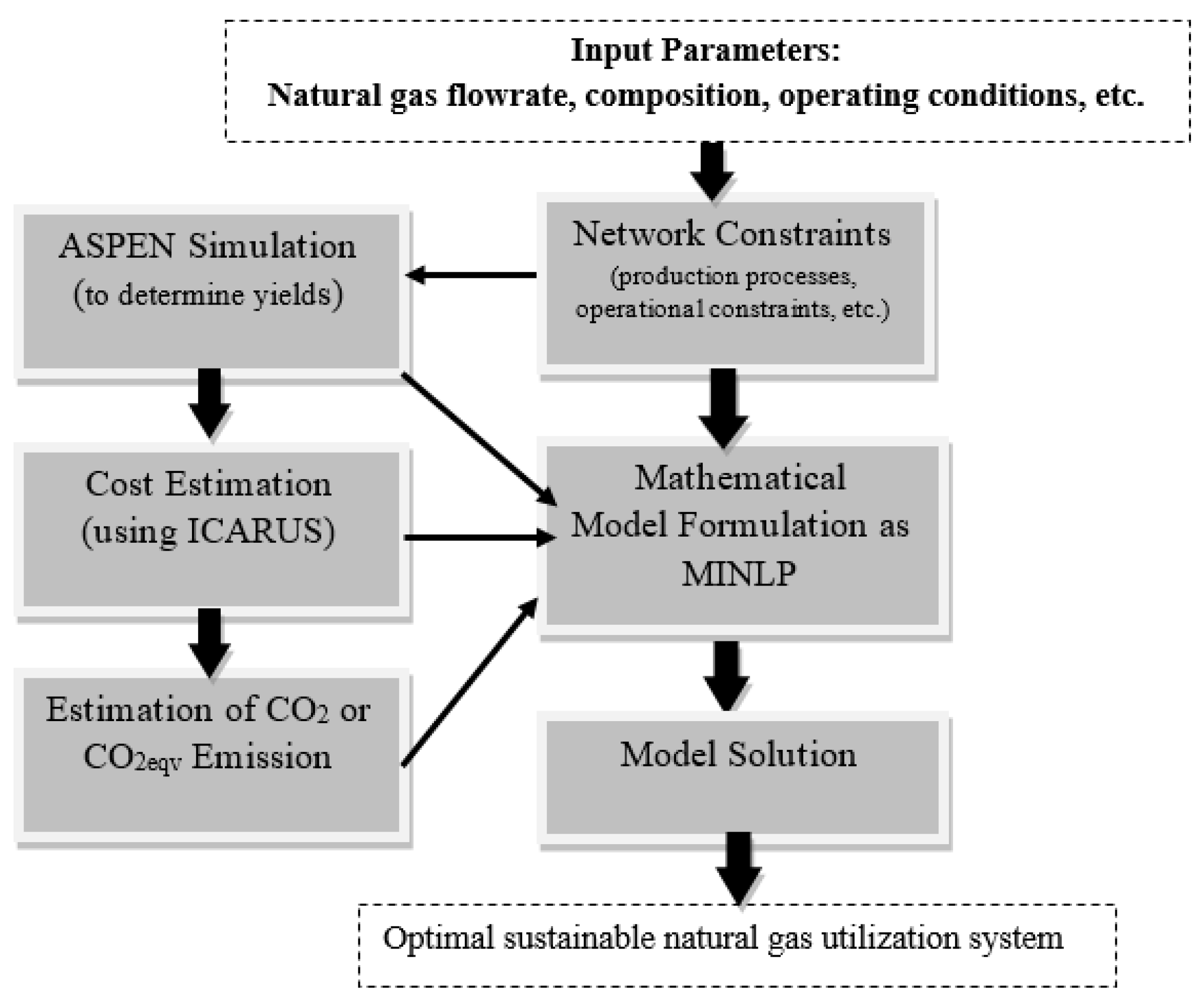
Given the operating flow rate range for natural gas, which is mainly composed of methane, there are different design alternatives and operating modes for each key processing unit in the natural gas downstream utilization network shown in Figure 1. Decision makers need to determine the optimal configuration to maximize production (e.g., product yields), minimize the total cost including capital investment and operating costs, with environmental consideration in terms of CO2 emissions for different alternative routes. Figure 2 illustrates the proposed overall methodology and solution strategy based on a sequential use of simulation and optimization for finding the economically optimal and environmentally sustainable configuration of a natural gas downstream utilization network. The different design alternatives shown in Table 1 are used to create the optimal superstructure design to produce LNG, GTL, and methanol products with respect to the specified network constraints for each unit.
It is important to fix the overall process structure, otherwise, many conversion processes need to be considered. For example, we can extend the overall process structure to consider the production of gasoline from the methanol product.
The ASPEN Plus [34] simulation package is used to find the yields for different production processes under various technology options and operating modes. It is worth mentioning that the selection of the optimal technology for each key processing unit prior to simulation stage takes into consideration of some factors such as: possible flow rate, composition, pressure, and temperature of feedstock, specification levels for product purity, and capital and operation costs for each process. The capital and operating costs are estimated using ASPEN’s cost estimator option, ICARUS. The environmental impact represented in the analysis by CO2 or CO2eq emission is also obtained using the ASPEN Plus simulator for each flowsheet configuration under different operating modes. Then we use all the above information to formulate and solve an MILP model for convergence to maximize the net profit.
4. Mathematical Programming Model
The proposed MILP formulation for optimizing the superstructure design includes an objective function that maximizes a weighted sum of the revenue, setup/operating costs, and cost of CO2 emission with constraints for minimum coverage level of energy demand, operational restrictions, and other limitations. In the mathematical model, the operations and associated material flow in each block of the natural gas utilization superstructure (specified in Table 1) are represented by constraints based on factors such as overall mass balance, yields, product quality requirements, available technologies, demand, and capacities. is a binary decision variable specifying the selection of technology and operating mode for each unit where and refer to sets of design alternatives and operating modes, respectively. That is:
4.1. Overall Mass Balance and Yield Model
In this section, we present the overall mass balance and product yield equations for each key processing unit in the considered superstructure starting with the syngas preparation unit. The methane-rich stream of natural gas feedstock,, is sent to both syngas preparation () and liquefaction units () simultaneously under technology option j and operating mode m. The exact percentage of methane fed to each unit is determined by optimization. However, lower bound values are set for both units to ensure that they are both operational. The overall mass balance of methane-rich stream can be expressed as:
The flow-balance constraints in the model guarantee that or for only one j and m couple through the following equation because only one reforming technology and operating mode can be selected among the available options.
where JA ≡ set of reforming technologies and MA ≡ set of operating modes for reforming technologies.
Although other technologies are available to produce syngas from natural gas, we will consider only ATR and SMR as competing technologies for the reforming unit due to their applicability in large scale production. The methane-rich stream directed to syngas unit ( is fed along a flow of steam with rate in the case of SMR, and with a flow of steam and oxygen with rates and in the case of ATR to produce the required syngas ratio. We define different balance equations for each technology by differentiating the associated flowrates with index j {ATR, SMR}. Output of each option is H2, CO and CO2 as shown in Equations (8)–(22) with different flowrates based on yield rates , associated with technology option j and operating mode m. Accordingly, we get different syngas (H2/CO) ratios based on technology and operating model selections. For instance, the desirable composition of the syngas for the low-temperature FT corresponds to a H2/CO ratio of two. The general syngas flowrate is defined in Equations (6) and (7):
For j = SMR, the overall material balance is given in Equations (8)–(13) where and are the upper bound for methane and steam streams. Equation (13) indicates the required steam flowrate for SMR technology as a function of methane flowrate derived via a simulation analysis with ASPEN Plus:
For j = ATR, the overall material balance is given in Equations (14) to (22) where is the upper bound for O2 stream. The operating steam-to-CH4 ratio is set to 0.6 as shown in Equation (21). This ratio, which is low compared to those used in previous studies (e.g., between 1.3 and 2.0), becomes the state-of-the-art syngas ratio for FT application in modern plants in Europe and Middle East [35].
Equation (22) states that the required oxygen flowrate is a function of methane flowrate. In order to produce the required syngas ratio, we need to generate O2 and CH4 flowrate data from the simulation and get different syngas ratio values by changing oxygen flowrate for a given methane flowrate. Then, by plotting syngas ratio vs. O2 flowrate, we can find the right value of O2 that corresponds to a syngas ratio of two, for which the sensitivity analysis modeling option of ASPEN Plus was used as discussed in Alsobhi et al. [7]. Note that in the above formulation, constraints Equations (11)–(12), Equations (18)–(20) ensure that outflow from Unit (A) is specified according to the technology selection for this unit.
The syngas produced in Unit (A) is distributed among the downstream candidate units namely, hydrogen unit (D), FT synthesis unit (E), and methanol synthesis unit (F) as shown in Equation (23). Again the amount of fed to these three units under technology option j are optimization variables, i.e., , respectively. The lower bounds on the required demand coverage guarantee that all three units receive syngas inflows:
The flow is used to produce hydrogen in Unit D based on the selection of hydrogen production technology and mode denoted by variable . Equation (25) ensures that only if technology j and operating mode m are selected, where represents an upper bound. Given the technology/mode selection and the amount of syngas fed to Unit (D), the associated H2 production is specified in Equation (26):
where, JD ≡ set of hydrogen production technologies and MD ≡ set of operating modes for hydrogen production technologies.
Another portion of the syngas produced in unit A, i.e., is fed to Unit E for FT synthesis. Based on the selection of the best technology/mode options, the corresponding syncrude production rate is specified by the yield rate . Produced syncrude is sent to Unit G for LPG, gasoline, diesel, and wax production:
where JE ≡ set of FT production technologies and ME ≡ set of operating modes for FT production technologies.
The rest of the syngas is fed to Unit F for methanol synthesis based on the following definition and constraints, which are similar to those for Unit (E):
where JF ≡ set of methanol production technologies and MF ≡ set of operating modes for methanol synthesis technologies.
The methane-rich stream fed to Unit (B) for liquefaction, , is compressed and cooled down to −160 °C. The output flow from Unit (B) is a liquid form of CH4 with some nitrogen content, . Therefore, the liquid CH4 is sent to Unit C for N2 rejection to produce an LNG stream, . Note that we consider a given technology and mode for Unit (C), therefore, Unit (C) does not have separate technology/mode variables and associated constraints. The process flow and mass-balance conditions for Unit (B) and (C) are expressed in the following definitions and constraints given; (i) and are the flowrate for fed N2 and produced LNG; and (ii) is the combined yield rate for both Units (B) and (C) under technology selection j and operating mode m in Unit (B). Equation (37) indicates the flowrate of N2 fed to Unit (B) as a function methane flowrate, which is calculated based on ASPEN Plus simulator:
where JB ≡ set of liquefaction technologies and MBF ≡ set of operating modes for liquefaction technologies.
The methanol crude and water composition produced in Unit (F) and syncrude produced in Unit E are sent to Unit (G) and (H), respectively, to produce associated final products. Note we consider fixed technology and mode options for Units (G) and (H). Equations (39)–(43) give the overall material balances around these two units, where sf1, sf2, sf3 and sf4 are pre-specified selectivity factors for LPG, gasoline, diesel, and wax, respectively:
4.2. Supply and Demand Constraints
Consumption of methane-rich feedstock through the network should be within the specified lower and upper bounds:
The annual demand constraints for the main products are given in Equations (45) to (51). Basically, these inequalities ensure that the annual production amounts are sufficient to cover the annual expected demand for LNG, H2, methanol, LPG, gasoline, diesel, and wax:
4.3. Capacity Constraint for Processing Units
Capacity constraints for main processing units of the production network are given in Equations (52)–(59) where , denotes the upper capacity limit for each Unit i, in technology j , and mode m . The capacity limits for Unit (G) and (H) are defined as and respectively, because these units are associated with a single technology and model option. These constraints limit the total inflow to each unit to ensure convergence of the mass flow. The necessary capacity limits are selected for a single production train, such as so that mass flow convergence is achieved in the ASPEN Plus Simulator:
4.4. Objective Function
The objective of the proposed optimization model is to maximize a utility function which is the sum of annual profit of production network and weighted annual CO2 and CO2eq emission amounts. The weight on the annual emission, we, has two functions: (i) Specifying the scenarios that consider only the total profit associated with the alternative production network designs i.e., we = 0; (ii) Specifying the penalty cost of CO2 emission for the scenarios that consider sustainability of the alternative production network designs as well, i.e., we > 0. The emission costs can be estimated from IEA [36] and BP [37]. We use the estimated emission costs for sensitivity analysis in Section 5.1 and Section 5.2. The total production cost is represented by the sum of annualized capital cost (), variable annual operating costs, and fixed annual operating cost () of Units (A) to (H) plus the annual cost of methane-rich feedstock stream usage. It is assumed that capital costs are amortized over the lifetime of the project life of 20 years with 10% as a compound interest rate. This compound interest rate represents a reasonable minimum rate of return expected from an investment alternative. The optimization model can be represented as follows:
s.t. constraints (4)–(59), and all variables are non-negative.
In this model, P = {LNG, H2, methanol, LPG, Gasoline, Diesel, Wax} refers to the set of final products. Parameters and refer to the sale price of one unit of product k and unit cost of natural gas feedstock. The resulting CO2 emission (i.e., ) for each unit, technology/mode option is derived from the ASPEN Plus Simulator.
5. Case Study
An illustrative case study is presented to show the applicability of the overall modeling framework considering both the scenarios of we = 0 and we > 0. Different rigorous simulations of the natural gas downstream utilization pathways were carried out using Aspen Plus to obtain surrogate models or appropriate yield equations for the production flowrates. We applied simulation analyses to the key processing units analyzed in this case study including: syngas preparing unit (A); liquefaction unit (B); N2 rejection unit (C); hydrogen unit (D); FT synthesis unit (E); methanol synthesis unit (F); FT upgrade unit (G); and MeOH upgrade unit (H). The methane-rich stream comes from an upstream network as described in Al-Sobhi et al. [8] with specified flowrate range and operating conditions. The cost data used in this case study is adapted from EIA [38] and is shown in Table 2. The yield values from ASPEN simulations are reported in Table 3. The demand (minimum and maximum), capacity, and the optimal solution of LP model of Al-Sobhi and Elkamel [7] is also reported for reference.
We first present some of the results from the simulation analysis with Aspen Plus to illustrate the yield values we used for the key production units, and the results of the overall framework when we focus on a single product (e.g., LNG, GTL, or methanol) at a time. For these single-product scenarios, we assumed utilization of the available methane stream at different percentages. First, we assumed that LNG is the most promising option and 100%, 70%, 50%, and 30% of methane stream is utilized to produce just LNG. Table 4 shows the total capital cost, total operating cost, total utilities cost, yield values, and objective function values for each planning mode considering LNG production. We repeated a similar analysis when and 100%, 70%, 50%, and 30% of methane stream is utilized for only methanol production whose results are summarized in Table 5.
Finally, we assume 100%, 70%, 50%, and 30% of methane stream is utilized to produce just FT (GTL) products. For FT processes, we have two distinct operating modes such as LTFT and HTFT. Table 6 and Table 7 show the results for these two operating modes, respectively.
As it can be observed from these tabulated results, $196 million, $1100 million, $1780 million, $282 million are the objective function values (profit) for 100% utilization methane stream for LNG, methanol, GTL via LTFT, and GTL via HTFT production, respectively. However, the results in the above tables imply that a higher profit can be achieved by allocating the methane stream to produce multiple end products. For example, (30% LNG, 70% GTL via HTFT) results in $2035 million, while (50% HTFT, 50% LNG) and (50% methanol, 50% GTL via HTFT) combinations result in $1502.6 million and $1978 million, respectively. These results illustrate the need for quantitative and systematic methods to derive the best combination of methane-rich feedstock utilization modes to achieve the optimal profit level. The proposed MILP model in Section 4 serves to this purpose.
5.1. Economic Planning Using Formulated Model
We also conduct an experiment with the MILP model for determining the optimal methane-rich feedstock utilization and production plan for the entire network to maximize the total profit, i.e., we = 0. The results of this numerical experiment illustrate the benefits of the proposed modeling framework in improving the efficiency of overall production pathways. Based on the different yields obtained for different products and different capital/operating costs for each utilization option, the formulated model was applied on the production network. After eliminating redundant and unbinding constraints, we solved the MILP model for 24 continuous variables, 4 integer variables, and 39 constraints using LINGO 14.0 version [39] with branch and bound solver type. We found that the total optimal profit is $4200 million when 196,079 kg/h of the methane-rich feedstock is used for methanol production, and 1,003,921 kg/h of it is used for GTL production via HTFT, i.e., the optimal production combination is (16% methanol, 84% HTFT). This optimal production combination produces a product flowrates of 130,817, 66,094, 299,854, 200,000, 200,784 kg/h for methanol, LPG, gasoline, diesel, and wax, respectively.
5.2. Sustainable Planning Using Formulated Model
The economic and environmental impacts are both important aspects to be considered when designing the natural gas utilization network and planning the optimal production pathways. In the literature, the environmental impacts are usually represented by CO2 or CO2eq emission amounts which are incorporated into this analysis. First of all, the CO2eq values for each utilization mode is obtained from the ASPEN Plus simulator. The greenhouse gas (GHG) emissions (carbon dioxide, methane, nitrous oxide, hydrofluorocarbons, perfluorocarbons, sulfur hexafluoride, and nitrogen trifluoride) are reported in ASPEN Plus in terms of CO2 equivalents of global warming potential (GWP) for the streams based on data from popular standards: IPCC’s 2nd (SAR), the 4th (AR4) assessment reports, and the U.S. EPA’s proposed rules from 2009 (ASPEN Plus V7.3 documentation). In our analysis, we consider the base case carbon cost as we = $40 per ton of CO2 equivalent emitted for the base case [37]. Then, different carbon prices such as we = $20 (low), and we = $80 (high) are considered to address possible scenarios for foreseeable variation in regulations of greenhouse gas emission. Table 8 shows the CO2 equivalent values in tons/year for different utilization options considering SAR standard with the base case carbon cost.
Now, the process with positive values will be discredited for carbon equivalent cost and a negative value will be added as operating cost and will be shown in their profit equation as they are emitting GHG according to their corresponding ASPEN Plus flowsheet. Whereas, the process with negative values will be credited for carbon equivalent cost and a positive cost will be shown in their profit equation as their output product streams are emitting less CO2 equivalent than their inputs streams according to their corresponding ASPEN Plus flowsheet.
After incorporating carbon equivalent cost value of $40 per ton emitted, it was found that $4165 million is the optimal annual profit as defined by the objective function. The optimal solution still selects methanol and GTL via HTFT combination with 196,079 kg/h and 1,003,921 kg/h, respectively. This is (16% methanol, 84% HTFT) as a production mix. Furthermore, the optimal solution does not change when the carbon emission cost is set to $20 or $80 per ton. We found that $4183 million and $4127 million are the optimal annual profit for (16% methanol, 84% HTFT) when CO2 emission cost is set to $20 and $80 per ton, respectively.
6. Conclusions
A novel natural gas production unit has been synthesized and analyzed. ASPEN Plus simulation package showed to be beneficial in calculating mass and energy balances accurately and finding the different yield equations. Then, the developed comprehensive mixed-integer linear programming (MILP) model has been implemented for the design and optimization of methane processing network. Our results provide several insights for the natural gas processing industries.
First of all, our results illustrate that when processing methane the technology selection and finding the optimal product combination is critical for profitability. That is, focusing only a single product in a facility is suboptimal. Furthermore, we show that the proposed MILP framework can effectively find the optimal production pathways on a realistic case study. From only profit maximization perspective, the optimal annual profit of the case study is $4200 Million with a product combination of (16% methanol, 84% HTFT). When we incorporated the carbon equivalent cost values, the optimal production pathway and technology selections did not change. This may indicate that the current carbon emission penalties may not be effective in leading natural gas processing industry towards seeking more environment friendly production network designs.
In the current version of the paper, we conducted extensive sensitivity analyses on % utilization of feedstock, whose results are informative about the effect of changes on feedstock rates on the model outcomes. We have conducted another sensitivity analysis with respect to emission prices showing that the model outcomes are robust against fluctuations in emission costs. This result implies that, unless other costs are increased or selling prices are reduced significantly, the model will not suggest a more environment-friendly optimal design network design.
The proposed method may help industrial decision makers to derive more efficient and sustainable process designs for natural gas downstream utilization networks. In addition, it may also help public decision makers to design more effective penalty mechanisms to ensure compliance with the target CO2 emission levels.
Acknowledgment
The authors would like to acknowledge the financial support from NSERC and from Qatar University to conduct this research. A.E. and M.A.S. would also like to acknowledge the Gas Research Center (GRC) at the Petroleum Institute during the later stages of this research.
Author Contributions
S.A.A. and A.E. defined the problem & experimental setting, and develop the optimization model. S.A.A. gathered the necessary data, prepared simulation code, and conducted the numerical experiments. M.A.S. and F.S.E. finetuned the optimization model, and helped S.A.A. analyze and interpret the results. S.A.A., A.E., M.A.S., and F.S.E. contributed in the paper writing. M.A.S. and F.S.E. handled the paper revisions.
Conflicts of Interest
The authors declare no conflict of interest.
Nomenclature
| Sets |
| i {A,…,H} = processing units j = technology/configuration |
| m = operational mode |
| k = product = the set of technology/configuration for processing unit i = the set of operating modes for processing unit i, |
| Binary variables |
| = Binary variable for selection of technology j in processing unit i at operational mode m |
| Continuous variables |
| |
| |
| |
| Other Parameters |
| under technology j and operating mode m |
| of product k we = cost of CO2 emision CO2ijm = CO2 emision in unit i for technology j in operating mode m in operating mode m in operating mode m |
| Superscripts |
| L = lower bound |
| U = upper bound |
Acronyms
| CH4 | Methane |
| LNG | Liquefied natural gas |
| GTL | Gas to liquids |
| LP | Linear programming |
| MILP | Mixed integer linear programming |
| NLP | Nonlinear programming |
| MINLP | Mixed integer nonlinear programming |
| GHG | Greenhouse gas |
| CNG | Compressed natural gas |
| GTS | Gas to solid |
| GTW | Gas to wire |
| CBM | Coal bed methane |
| FT | Fischer-Tropsch |
| DME | Dimethylether |
| RWGSR | Reverse water gas shift reaction |
References
- Thomas, S. Review of ways to transport natural gas energy from countries which do not need the gas for domestic use. Energy 2003, 2814, 1461–1477. [Google Scholar] [CrossRef]
- BC Ministry of Energy and Mines. British Columbia’s Natural Gas Strategy Fuelling B.C.’s Economy for the Next Decade and Beyond; BC Ministry of Energy and Mines: Vancouver, BC, Canada, 2012. Available online: http://www.gov.bc.ca/ener/popt/down/natural_gas_strategy.pdf (accessed on 24 September 2017).
- BC Ministry of Energy, Mines, and Natural Gas. British Columbia’s Liquefied Natural Gas Strategy: One Year Update; BC Ministry of Energy, Mines, and Natural Gas: Vancouver, BC, Canada, 2013; pp. 1–16. Available online: https://lnginbc.gov.bc.ca/app/uploads/sites/16/2016/07/BCs-LNG-Strategy-One-Year-Update-2013_web130207.pdf (accessed on 24 September 2017).
- ExxonMobil. Outlook for Energy: A View to 2040; ExxonMobil: Irving, TX, USA, 2017; Available online: http://cdn.exxonmobil.com/~/media/global/files/outlook-for-energy/2016/2016-outlook-for-energy.pdf (accessed on 24 September 2017).
- Wood, D.A.; Nwaoha, C.; Towler, B.F. Gas-to-liquids (GTL): A review of an industry offering several routes for monetizing natural gas. J. Nat. Gas Sci. Eng. 2012, 9, 196–208. [Google Scholar] [CrossRef]
- Olah, G.A.; Goeppert, A.; Prakash, G.K.S. Beyond Oil and Gas: The Methanol Economy; WILEY-VCH: Weinheim, Germany, 2006. [Google Scholar]
- Al-Sobhi, S.A.; Elkamel, A. Simulation and optimization of natural gas processing and production network consisting of LNG, GTL, and methanol facilities. J. Nat. Gas Sci. Eng. 2015, 23, 500–508. [Google Scholar] [CrossRef]
- Al-Sobhi, S.A.; Shaik, M.A.; Elkamel, A.; Erenay, F.S. Integrating simulation in optimal synthesis and design of natural gas upstream processing networks. Ind. Eng. Chem. Res. 2017. [Google Scholar] [CrossRef]
- Rostrup-Nielsen, J.; Christiansen, L.J. Concepts in Syngas Manufacture; World Scientific: Singapore, 2011; Volume 10. [Google Scholar]
- Ramberg, D.J.; Chen, Y.H.H.; Paltsev, S.; Parsons, J.E. The economic viability of gas-to-liquids technology and the crude oil-natural gas price relationship. Energy Econ. 2017, 63, 13–21. [Google Scholar] [CrossRef]
- Aasberg-Petersen, K.; Bak Hansen, J.H.; Christensen, T.S.; Dybkjaer, I.; Christensen, P.S.; Stub Nielsen, C.; Rostrup-Nielsen, J.R. Technologies for large-scale gas conversion. Appl. Catal. A Gen. 2001, 221, 379–387. [Google Scholar] [CrossRef]
- Luyben, W.L. Design and Control of the Dry Methane Reforming Process. Ind. Eng. Chem. Res. 2014, 53, 14423–14439. [Google Scholar] [CrossRef]
- Rostrup-Nielsen, J.R. New aspects of syngas production and use. Catal. Today 2000, 63, 159–164. [Google Scholar] [CrossRef]
- Wilhelm, D.J.; Simbeck, D.R.; Karp, A.D.; Dickenson, R.L. Syngas production for gas-to-liquids applications: Technologies, issues and outlook. Fuel Process. Technol. 2001, 71, 139–148. [Google Scholar] [CrossRef]
- Rostrup-Nielsen, J.R. Syngas in perspective. Catal. Today 2002, 71, 243–247. [Google Scholar] [CrossRef]
- Aasberg-Petersen, K.; Christensen, T.S.; Nielsen, C.S.; Dybkjær, I. Recent developments in autothermal reforming and pre-reforming for synthesis gas production in GTL applications. Fuel Process. Technol. 2003, 83, 253–261. [Google Scholar] [CrossRef]
- Bakkerud, P.K. Update on synthesis gas production for GTL. Catal. Today 2005, 106, 30–33. [Google Scholar] [CrossRef]
- Julia, L.M.; Ortiz-Espinoza, A.P.; El-Halwagi, M.M.; Jime, A. Techno-Economic Assessment and Environmental Impact of Shale Gas Alternatives to Methanol. ACS Sustain. Chem. Eng. 2014, 2, 2338–2344. [Google Scholar]
- Noureldin, M.M.B.; Elbashir, N.O.; El-Halwagi, M.M. Optimization and selection of reforming approaches for syngas generation from natural/shale gas. Ind. Eng. Chem. Res. 2014, 53, 1841–1855. [Google Scholar] [CrossRef]
- Tusiani, M.; Shearer, G. LNG, A Nontechnical Guide; PennWell Corporation: Tulsa, OK, USA, 2007. [Google Scholar]
- Mokhatab, S.; Economides, M.J. Onshore LNG Production Process Selection. In Proceedings of the SPE Annual Technical Conference and Exhibition, San Antonio, TX, USA, 24–27 September 2006; Volume 1, pp. 1–11. [Google Scholar]
- International Gas Union (IGU). International Gas Union (IGU) World LNG Report; IGU: Barcelona, Spain, 2017. [Google Scholar]
- Kidnay, A.J.; Parrish, W.R. Fundamentals of Natural Gas Processing; Taylor & Francis: Boca Raton, FL, USA, 2006. [Google Scholar]
- Gas Processors Suppliers Association (GPSA). Engineering Data Book, 12th ed.; GPSA: Tulsa, OK, USA, 2004. [Google Scholar]
- Kuo, J.C.; Wang, K.H.; Chen, C. Pros and cons of different Nitrogen Removal Unit (NRU) technology. J. Nat. Gas Sci. Eng. 2012, 7, 52–59. [Google Scholar] [CrossRef]
- Mueller-Langer, F.; Tzimas, E.; Kaltschmitt, M.; Peteves, S. Techno-economic assessment of hydrogen production processes for the hydrogen economy for the short and medium term. Int. J. Hydrog. Energy 2007, 32, 3797–3810. [Google Scholar] [CrossRef]
- Silveira, J.L. Sustainable Hydrogen Production Processes: Energy, Economic and Ecological Issues; Green Energy and Technology Series; Springer: Cham, Switzerland, 2017. [Google Scholar] [CrossRef]
- Dry, M.E. The Fischer-Tropsch process: 1950–2000. Catal. Today 2002, 71, 227–241. [Google Scholar] [CrossRef]
- Steynberg, A.P.; Espinoza, R.L.; Jager, B.; Vosloo, A.C. High temperature Fischer–Tropsch synthesis in commercial practice. Appl. Catal. A Gen. 1999, 186, 41–54. [Google Scholar] [CrossRef]
- De Klerk, A. Fischer-Tropsch Refining; Wiley-VCH Verlag GmbH & Co. KGaA: Weinheim, Germany, 2011. [Google Scholar]
- Velasco, J.A.; Lopez, L.; Velásquez, M.; Boutonnet, M.; Cabrera, S.; Järås, S. Gas to liquids: A technology for natural gas industrialization in Bolivia. J. Nat. Gas Sci. Eng. 2010, 2, 222–228. [Google Scholar] [CrossRef]
- Espinoza, R.L.; Steynberg, A.P.; Jager, B.; Vosloo, A.C. Low temperature Fischer–Tropsch synthesis from a Sasol perspective. Appl. Catal. A Gen. 1999, 186, 13–26. [Google Scholar] [CrossRef]
- Jager, B.; Espinoza, R.L. Advances in Low-Temperature Fischer-Tropsch Synthesis. Catal. Today 1995, 23, 17–28. [Google Scholar] [CrossRef]
- ASPEN Plus V7.3; Aspen Technology, Inc.: Bedford, MA, USA, 2011.
- Steynberg, A.; Dry, M. Fischer-Tropsch Technology; Elsevier B.V.: Amsterdam, The Netherlands, 2004. [Google Scholar]
- International Energy Agency (IEA). World CO2 Emissions from Fuel Combustion Database Documentation; International Energy Agency: Paris, France, 2017. [Google Scholar]
- British Petroleum Company (BP). British Petroleum Statistical Review of World Energy; British Petroleum Co.: London, UK, June 2017. [Google Scholar]
- Energy Information Administration (EIA). Monthly Natural Gas Liquids Reports; Energy Information Administration: Washington, DC, USA, 2015.
- Linear, Interactive, and General Optimizer (LINGO) Software, LINDO System Inc.: Chicago, IL, USA, 2013.
Figure 1.
Superstructure representation for the considered natural gas downstream utilization network.
Figure 1.
Superstructure representation for the considered natural gas downstream utilization network.
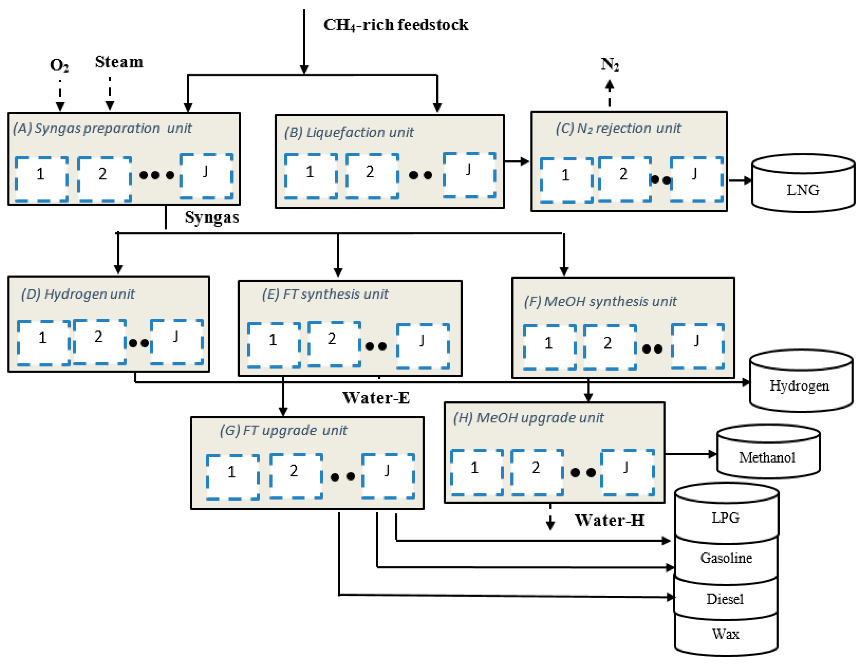
Figure 2.
General solution strategy for sequential use of simulation and optimization for natural gas utilization system.
Figure 2.
General solution strategy for sequential use of simulation and optimization for natural gas utilization system.


Table 1.
Different possible technologies & operating modes considered in the superstructure.
| Major Processing Unit (i) | Possible Processes/Technologies | Considered Technology | Operating Modes (Mi) |
| Syngas preparation unit (A) |
|
|
|
| Liquefaction unit (B) |
|
|
|
| N2 rejection unit (C) |
|
|
|
| Hydrogen unit (D) |
|
|
|
| FT synthesis unit (E) |
|
|
|
| Methanol synthesis unit (F) |
|
|
|
| Product upgrading unit (G&H) |
|
|
|
Table 2.
Economic Data [38].
Table 2.
Economic Data [38].
| Natural Gas Feedstock | $ 4.4 per MMBtu |
|---|---|
| LNG | $7 per thousand cubic feet |
| LPG | $2.5 per gallon |
| Gasoline | $2.8 per gallon |
| Diesel | $3 per gallon |
| Wax | $2 per gallon |
| Methanol | $500 per ton |
Table 3.
Yields and products flowrates obtained from simulation and LP model.
| Products | Natural Gas (kg/h) | Yield * | Min. Demand (kg/h) | Max. Demand (kg/h) | LP Model Output (kg/h) |
|---|---|---|---|---|---|
| LNG | 1,044,157 | 0.690 | 1,000,000 | 1,200,000 | 1,090,000 |
| Losses associated with LNG | 232,343 | 0.152 | 230,000 | 235,000 | 230,000 |
| LPG | 114,000 | 0.075 | 110,000 | 120,000 | 120,000 |
| Gasoline | 227,911 | 0.150 | 220,000 | 230,000 | 230,000 |
| Diesel | 174,730 | 0.110 | 170,000 | 180,000 | 180,000 |
| Wax | 99,900 | 0.070 | 95,000 | 100,000 | 100,000 |
| Losses associated with GTL | 735,159 | 0.480 | 733,000 | 735,200 | 733,000 |
| Methanol | 870,000 | 0.574 | 850,000 | 900,000 | 900,000 |
| Losses associated with methanol | 419,200 | 0.270 | 400,000 | 410,000 | 400,000 |
| Available NG supply (kg/h) | 1,515,000 | - | - | - | - |
* Yield defined as product flowrate divided by feedstock flowrate.
Table 4.
LNG production results for different methane feedstock utilization levels.
| LNG | 100% | 70% | 50% | 30% |
|---|---|---|---|---|
| Total capital cost, $M | 18.45 | 14.30 | 11.60 | 8.90 |
| Amortized capital cost, $M/year | 2.24 | 1.74 | 1.42 | 1.08 |
| Total operating cost, $M/year | 248.10 | 174 | 124 | 74.5 |
| Total utilities cost, $M/year | 229.60 | 161 | 115 | 18.9 |
| Desired rate of return, %/year | 10 | 10 | 10 | 10 |
| Lifetime of the project, year | 20 | 20 | 20 | 20 |
| LNG mass flow rate, kg/h | 1,128,350 | 789,845 | 564,175 | 338,505 |
| LNG yield | 0.88 | 0.62 | 0.44 | 0.26 |
| Objective function, $M | 196 | 134 | 92.60 | 51.10 |
Table 5.
Methanol production results for different methane feedstock utilization levels.
| Methanol | 100% | 70% | 50% | 30% |
|---|---|---|---|---|
| Total capital cost, $M | 44.8 | 33.7 | 25 | 19.3 |
| Amortized capital cost, $M/year | 5.45 | 4.10 | 3.04 | 2.35 |
| Total operating cost, $M/year | 71.5 | 58.5 | 50.4 | 42.3 |
| Total utilities cost, $M/year | 12.0 | 50.6 | 43.4 | 36.2 |
| Desired rate of return, %/year | 10 | 10 | 10 | 10 |
| Lifetime of the project, year | 20 | 20 | 20 | 20 |
| Methanol mass flowrate, kg/h | 688,053 | 481,615 | 344,011 | 206,401 |
| Water mass flowrate, kg/h | 480 | 336 | 240 | 144 |
| Methanol yield | 0.67 | 0.47 | 0.33 | 0.20 |
| Objective function, $M | 1100 | 845 | 568 | 291 |
Table 6.
GTL (LTFT) production results for different methane feedstock utilization levels.
| GTL LTFT | 100% | 70% | 50% | 30% |
|---|---|---|---|---|
| Total capital cost, $M | 86.4 | 64 | 44.0 | 30.4 |
| Amortized capital cost, $M/year | 10.5 | 7.8 | 5.35 | 3.7 |
| Total operating cost, $M/year | 31.6 | 22.9 | 16.2 | 10.6 |
| Total utilities cost, $M/year | 24.3 | 17.0 | 11.7 | 1.96 |
| Desired rate of return, %/year | 10 | 10 | 10 | 10 |
| lifetime of the project, year | 20 | 20 | 20 | 20 |
| LPG mass flowrate, kg/h | 12,850 | 4471 | 2725 | 2395 |
| Gasoline mass flowrate, kg/h | 83,664 | 57,696 | 41,179 | 27,773 |
| Diesel mass flowrate, kg/h | 162,909 | 114,612 | 76,502 | 40,226 |
| Wax mass flowrate, kg/h | 610,756 | 443,272 | 310,548 | 188,175 |
| Water mass flowrate, kg/h | 65,799 | 34,693 | 32,462 | 19,477 |
| LPG yield | 0.012 | 0.004 | 0.003 | 0.002 |
| Gasoline yield | 0.081 | 0.056 | 0.040 | 0.027 |
| Diesel yield | 0.158 | 0.111 | 0.074 | 0.040 |
| Wax yield | 0.592 | 0.430 | 0.301 | 0.182 |
| Objective function, $M | 1780 | 1400 | 935 | 513 |
Table 7.
GTL (HTFT) production results for different methane feedstock utilization levels.
| GTL HTFT | 100% | 70% | 50% | 30% |
|---|---|---|---|---|
| Total capital cost, $M | 90.5 | 57.7 | 47.2 | 34.4 |
| Amortized capital cost, $M/year | 11.0 | 7.02 | 5.74 | 4.18 |
| Total operating cost, $M/year | 4560 | 1510 | 1150 | 923 |
| Total utilities cost, $M/year | 4170 | 1400 | 1060 | 852 |
| Desired rate of return, %/year | 10 | 10 | 10 | 10 |
| lifetime of the project, year | 20 | 20 | 20 | 20 |
| LPG mass flowrate, kg/h | 67,898 | 308,035 | 202,597 | 205,452 |
| Gasoline mass flowrate, kg/h | 308,035 | 223,772 | 136,950 | 137,400 |
| Diesel mass flowrate, kg/h | 202,597 | 158,931 | 103,560 | 94,112 |
| Wax mass flowrate, kg/h | 205,452 | 77,533 | 50,213 | 47,776 |
| Water mass flowrate, kg/h | 124,745 | 87,321 | 62,504 | 61,502 |
| LPG yield | 0.066 | 0.299 | 0.196 | 0.199 |
| Gasoline yield | 0.2987 | 0.217 | 0.133 | 0.133 |
| Diesel yield | 0.196 | 0.154 | 0.100 | 0.091 |
| Wax yield | 0.199 | 0.075 | 0.049 | 0.046 |
| Objective function, $M | 282 | 1960 | 1410 | 1480 |
Table 8.
CO2 equivalent values in tons/year for different utilization options.
| Utilization Option/Percentage | 100% | 70% | 50% | 30% |
|---|---|---|---|---|
| LNG | 0.01471095 | −7.23 × 10⁷ | −1.21 × 10⁸ | −1.69 × 10⁸ |
| Methanol | −1.14 × 10⁴ | −7.95 × 10³ | −5.68 × 10³ | −3.41 × 10³ |
| LTFT | 3.94 × 10⁵ | 1.57 × 10⁵ | 1.96 × 10⁵ | 1.17 × 10⁵ |
| HTFT | 1.94 × 10⁶ | 1.36 × 10⁶ | 9.72 × 10⁵ | 9.95 × 10⁵ |
© 2018 by the authors. Licensee MDPI, Basel, Switzerland. This article is an open access article distributed under the terms and conditions of the Creative Commons Attribution (CC BY) license (http://creativecommons.org/licenses/by/4.0/).
Share and Cite
MDPI and ACS Style
Al-Sobhi, S.A.; Elkamel, A.; Erenay, F.S.; Shaik, M.A. Simulation-Optimization Framework for Synthesis and Design of Natural Gas Downstream Utilization Networks. Energies 2018, 11, 362. https://doi.org/10.3390/en11020362
AMA Style
Al-Sobhi SA, Elkamel A, Erenay FS, Shaik MA. Simulation-Optimization Framework for Synthesis and Design of Natural Gas Downstream Utilization Networks. Energies. 2018; 11(2):362. https://doi.org/10.3390/en11020362
Chicago/Turabian StyleAl-Sobhi, Saad A., Ali Elkamel, Fatih S. Erenay, and Munawar A. Shaik. 2018. "Simulation-Optimization Framework for Synthesis and Design of Natural Gas Downstream Utilization Networks" Energies 11, no. 2: 362. https://doi.org/10.3390/en11020362
Note that from the first issue of 2016, this journal uses article numbers instead of page numbers. See further details here.