Article

An Analysis for the Influences of Fracture Network System on Multi-Stage Fractured Horizontal Well Productivity in Shale Gas Reservoirs

1
PetroChina Southwest Oil & Gas Field Company, Chengdu 610000, Sichuan, China
2
Petroleum Engineering College, Southwest Petroleum University, Chengdu 610500, Sichuan, China
3
PetroChina Tarim Oilfield Company, Korla 841000, Xinjiang, China
*
Author to whom correspondence should be addressed.
Energies 2018, 11(2), 414; https://doi.org/10.3390/en11020414
Submission received: 25 January 2018 / Revised: 3 February 2018 / Accepted: 6 February 2018 / Published: 11 February 2018

Abstract

:
This paper presents two representative models to analyze the flow dynamic of multi-scale porous medium in hydraulic fractured horizontal shale gas wells. In this work, considering the characteristic mechanisms (multi-scale porous space, desorption and diffusion), flow equations in shale are established. After that, two representative models (discrete fracture model and dual-porosity model) are tailored to our issues. Solved by the control-volume finite element method (CVFEM), influences of fracture network system on productivity in shale reservoirs are analyzed in detail. Based on the analysis, the effects can be summarized as follow: at the beginning of production, high conductivity fracture network means more free gas could be produced; at the later part of production, high conductive fracture network can form a large low pressure region, which can not only stimulate the desorption of adsorbed gas, but also reduce the flow resistance to the well. Finally, the sensitivities of characteristic parameters in shale are discussed.

1. Introduction

Shale gas reservoir is a typical unconventional resource, which has played an irreplaceable role in world energy consumption since the beginning of this century. The reservoir is characterized by self-sealing and self-sourcing, multi-scale porosity and extremely tight matrix with ultra-low permeability. Moreover, proven by huge amount of field practices, fractured horizontal well could be the only way to obtain commercial production from shale gas reservoir [1,2]. In recent years, with the consideration of complex boundary constraints, dual-storage and multi-scale seepage mechanisms, flow dynamic models of fractured horizontal wells in shale gas reservoir are presented by many scholars. However, as a significant indicator of production rate, fracture network system still need comprehensive discussions. In this paper, based on the previous studies of multi-scale storage and seepage mechanisms and considered representative fracture network models, the partial differential flow equations in shale gas reservoirs are established. Then, with the combination of control-volume finite element method (CVFEM) numerical solution [3] and discrete fracture network algorithm, the production decline curves and pressure transient distributions are obtained. After that, the influences of diffusion, adsorbed gas, Langmuir volume and net-fracture system on production performances are analyzed. In particular, this paper focuses on the discussions about fracture network system.
Different from conventional reservoirs, the pore diameter distribution in shale is characterized by a bimodal curve occuring in the 10–1000 nm range [4]. Due to the brittleness of shale, after stimulation operation, fracture network system would become an indispensable part of the porosity. Obviously, the multimodal pore space may lead to the multi-mechanisms and complicated state equations of the gas flow in shale, such as ad-desorption, diffusion, slippage and stress sensitivity.
As reported, in shale formations, natural gas is generally trapped as both free gas and adsorbed gas [5]. The existence of kerogen and higher contents of clay minerals in shale has undoubtedly caused the larger surface of nanopores [6,7]. In contrast to conventional reservoirs, the content of gas adsorbed on the surfaces might be up to 85%, while the other 15% is held as free gas in macropore spaces [8]. More importantly, according to Mengal’s research [9], during the production period, the adsorbed gas can be extracted through the pressure depletion, which is an important contribution to keep the steady productivity in later period. In recent works, scholars [10,11,12] hold out that the ad-desorption theory in some shale should be described by the Brunauer-Emmett-Teller (BET) isotherm. However, in this paper, the ad-desorption law conforms to the Langmuir formula, which is proven by most observations [13,14,15,16].
Since the nanopore volume contributes the majority of shale porosity, gas flow in shale matrix should be described by multi-mechanisms (Figure 1). Ertekin et al. (1986) establish a dual mechanism model to describe the fluid flow in tight porous media [17]. Comparing the Fick diffusion with the Klinkenberg equation, the gas flow in micropores is calculated by a dynamic apparent permeability factor. Many studies adopted a similar idea to model shale gas seepage mechanisms by modified apparent permeability coefficient. According to the definition, Roy and Raju (2003) obtained the Knudsen number by calculating the ratio of the gas molecular mean free path and shale pore radius [18]. The results show that the slip flow and transitional flow are the typical flow regime in shale, which is different from the linear flow equation of conventional gas reservoirs. Ozkan et al. (2010) studied the flow mechanisms in shale matrix and micro fracture system [19], and developed a dual-mechanisms model by coupling diffusion with Darcy flow to describe the gas flow in shale matrix.
Javadpour et al. (2007) put forward an improved method for the Knudsen number calculation [20]. Then, the flow regimes are classified through the improved formula. Considering shale pore structures with the calculated results, Javadpour (2009, 2013) presented a gas apparent permeability to describe the seepage mechanism in nano-pore [21,22], which is a combination of viscous flows and Knudsen diffusion. Civan (2010, 2011, 2013) used a simplified second-order slip equation and several empirical parameters to model a seepage permeability formula in tight porous media, and by incorporating the Knudsen diffusion into the slippage equation [23,24], an apparent permeability formula for shale gas reservoir was proposed [25]. According to Javadpour’s results, Swami and Settari (2012) coupled Darcy flow, Knudsen diffusion and slip flow to establish the nano-scale seepage mechanism in shale [26]. As shown by the calculations, the apparent permeability of shale gas reservoir increased with the pressure depletion, which indicates the multi-mechanism has important influence on the later production period. Based on molecular dynamic theories, Deng et al. (2014) proposed a multi-mechanism model considering the gas diffusion, slippage effect and adsorption desorption by solving the Beskjok–Kaeniadakis equation [27]. The permeability is treated as a function of the adsorption layer, which is not easy to determine for field practices. According to historical works, gas diffusion, slip flow, and Darcy flow, as the main flow regimes of gas flow in shale, are considered in this paper. Moreover, to facilitate the calculation, the apparent permeability is derived as a function of the Knudsen number.
Shale formations have a high content of lime, mica, calcareous and other brittle minerals. Take the Longmaxi formation, a representative shale formation in the Sichuan basin, as an example, the average brittle mineral content is up to 60%. After hydraulic stimulation, the structural fractures, shrinkage fractures and overpressure fractures can be connected by the artificial fractures. The widely distributed fracture network system with high conductivity is defined as the stimulated reservoir volume (SRV), which plays a significant role for commercial production in unconventional reservoirs. Thus far, different methods are used by scholars to study the influences of the SRV in shale. Wu (2009) established a triple-porosity model to describe the gas flow in shale [28]. In this model, the stimulated reservoir is divided into micro and macro fracture system. Through detailed analysis, the effects of SRV system on economic benefits in unconventional reservoirs are revealed; however, un-stimulated zone and characteristics flow mechanisms of shale fail to be discussed. Based on the classical Warren–Root dual-porosity model, an equivalent Multi-stage fractured horizontal (MFH) model in shale [29] is presented by Bello and Watenbargen (2010). Although the flow regimes and production dynamics is discussed in detail in the work, the diffusion and adsorption effects in shale are neglected. Moreover, the model assumes that linear flow is the only regime in MFH well, which is not accurate and could lead to an unconvinced result in radial or elliptic flow periods. Since the linear flow assumption is convenient for derivation and solution, the linear flow model is widely used for research on unconventional reservoir [30,31,32,33]. In fact, because of the early flow around fractures is linear, the linear flow results are in good agreement with the accurate solutions in the early period of time. Nevertheless, the existence of fracture with high conductivity makes the duration of the linear flow not assumable. Therefore, the liner flow model is more suitable to describe the flow in homogeneous and unconventional reservoirs without fracture network system. To overcome this limitation, scholars try to study the gas flow through numerical simulation. With the consideration of multi-scale flow mechanisms and ad-desorption, Jiang (2015) used dual permeability model to characterize the production dynamic in shale [34]. The results show that the desorption gas is an important production supplements in low pressure period. Wang (2015) used finite difference method to solve a MFH well flow model in shale [35]. The model combines the slippage effect, viscous flow and Knudsen diffusion mechanism of shale gas reservoirs. The calculation indicates that the fracture network system could form a low pressure area in shale reservoirs which can stimulate the gas desorption. Although the literature presents several significant and useful suggestions to shale reservoirs development, limited by the orthogonal grids, conventional bi-wing fracture and explicit algorithm, the contribution of fracture network system for gas extraction is still lacking from the discussion.
In this paper, to study the influences of characteristic mechanisms on flow dynamic in shale, the models give a comprehensive consideration of multi-scale flow mechanisms, such as diffusion flow, desorption and slippage flow. More significantly, both discrete fracture model and dual-porosity model are presented to elaborate the stimulation of fracture network for the gas flow rate (Figure 2). Then, with the assistances of unstructured grids, district fracture network (DFN) model and control volume finite element method (CVFEM), the flow equations are solved implicitly. Ultimately, the influences of characteristic parameters on production rate are discussed by sensitivity analyses, which provide some insights into the study of flow dynamic in shale.

2. Mathematical Model

2.1. Model Assumption

To describe the gas flow in shale, some idealizations and assumptions are made (Figure 3):
(1)
The model is derived for single-phase isothermal gas flow in shale.
(2)
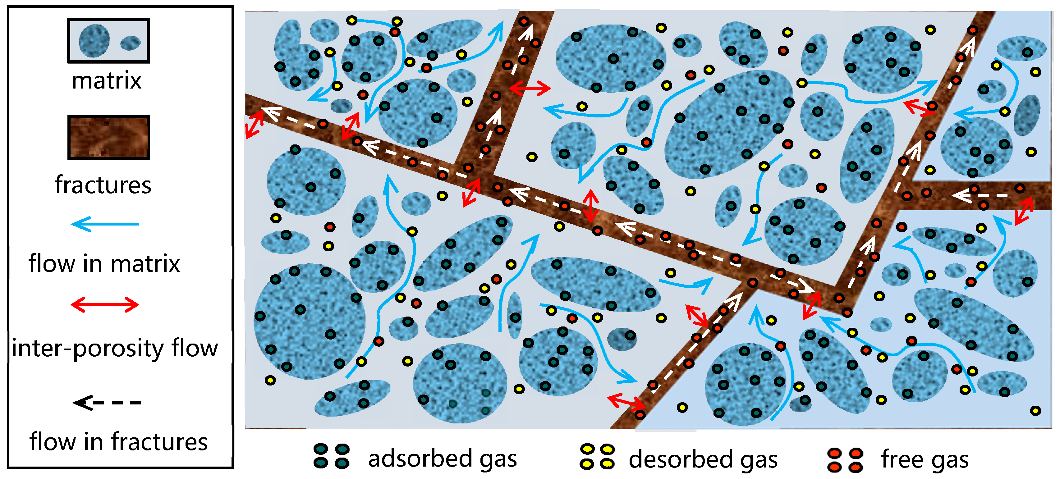
Both natural fractures and hydraulic fractures are main flow paths, and filled with the free gas. Additionally, shale matrix is filled with part of the free gas and almost all of the adsorption gas.
(3)
The inter-porosity flux between shale matrix and fracture system is described by the pseudo-steady mechanism.
(4)
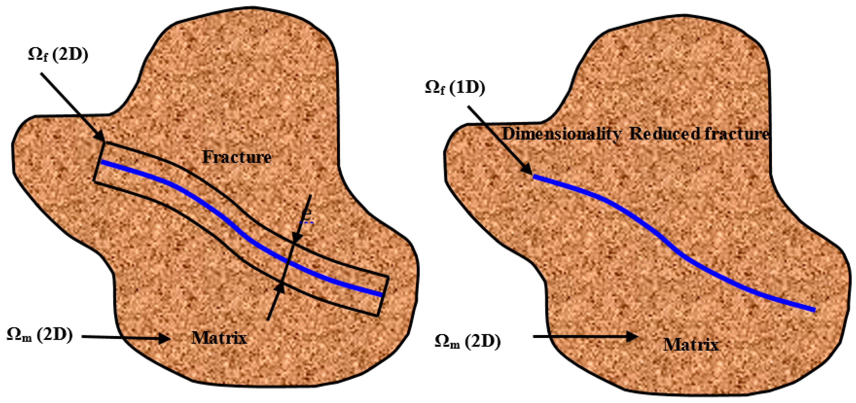
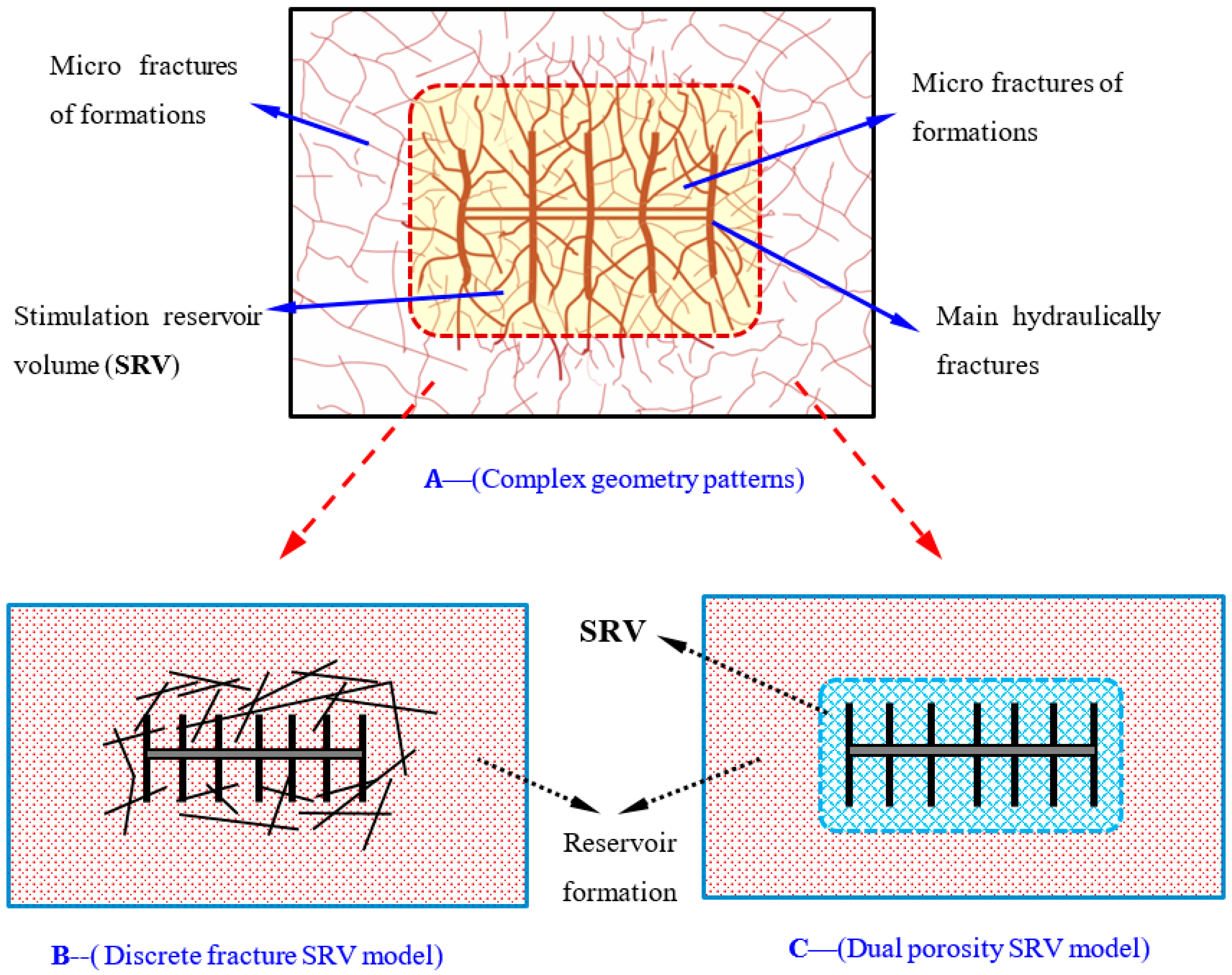
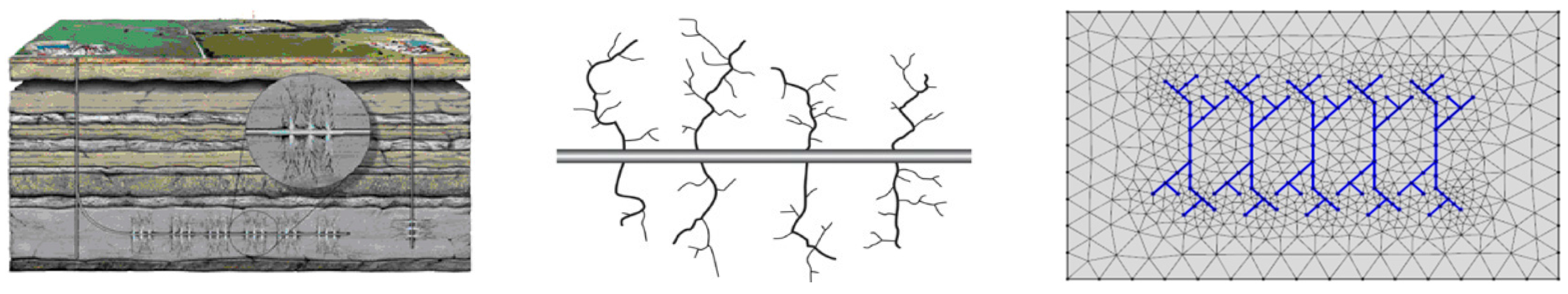
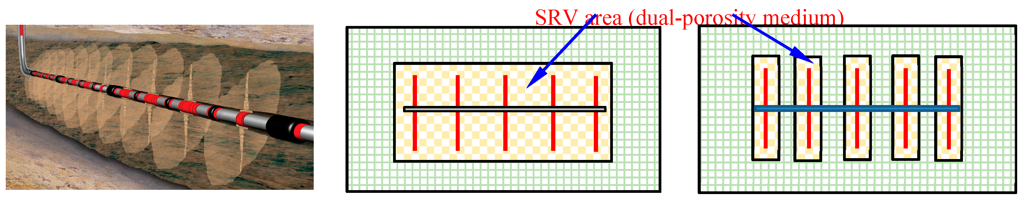
With the consideration of the stress sensitivity, a dual-porosity composite model and a DFN model are established to reflect the effects of fracture networks.
(5)
The main hydraulic fractures are assumed to be finite-conductivity.

2.2. Adsorption/Desorption

According to the similarity of coalbed methane, scholars have long noticed that the adsorption gas is a significant feature in shale. As Hill reported [8], approximately 30–60% of the gas occurs by adsorption mechanism. Based on the analysis of experiments, the majority of current research uses Langmuir’s isotherm to describe the adsorbed gas [36,37,38,39]. Moreover, the theory is also adopted in many commercial simulators [40]. As the Langmuir equation shows, under constant temperature condition, the relationship between gas pressure and adsorbed volume can be expressed as:
V E = V L p p L + p
where VL and PL are the Langmuir volume and Langmuir pressure, respectively, which represent the adsorption capability and reflect the characteristic of the curve.

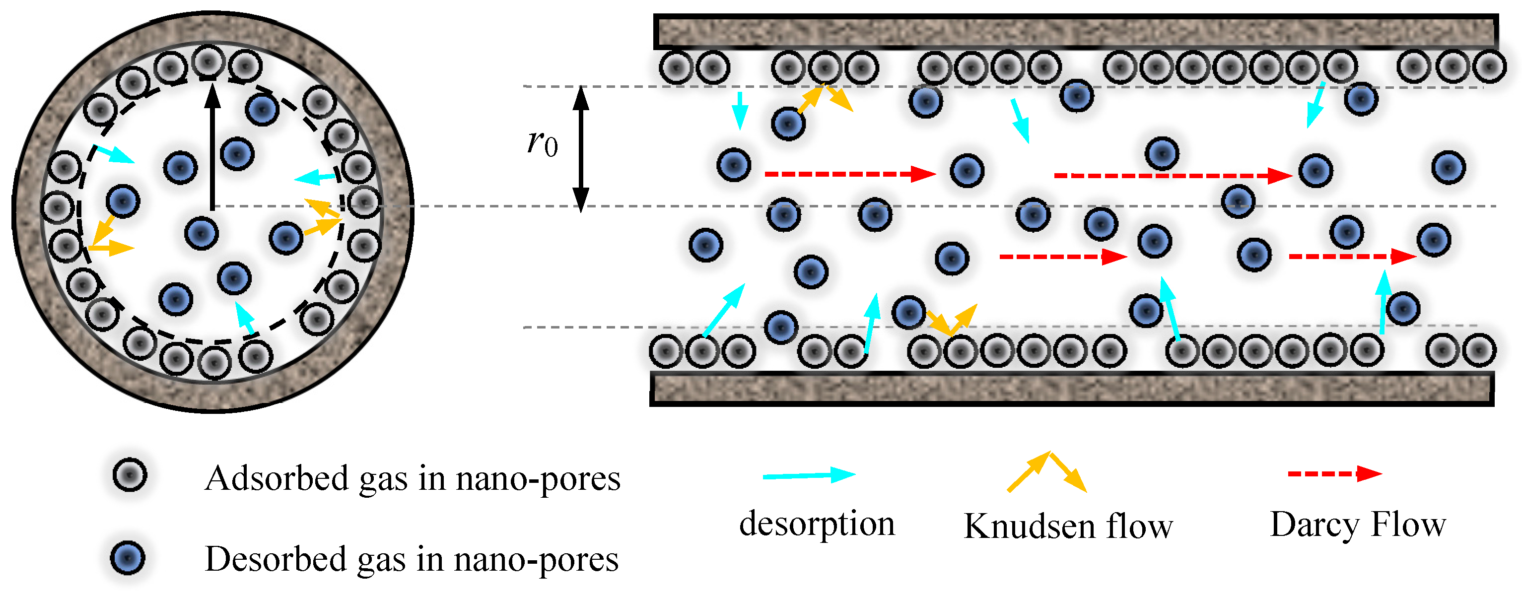
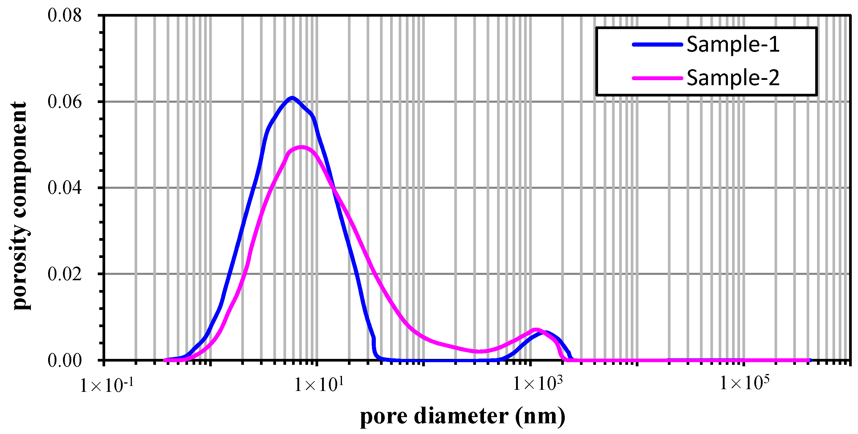
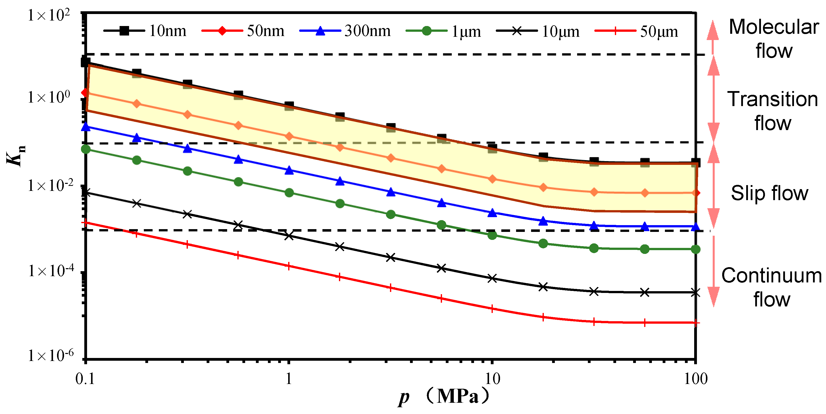
2.3. Flow Regimes and Mechanisms in Micro-Pores

Historic research of shale pore structures reveals that the pore distribution is bimodal. Figure 4 shows representative pore distributions curves of Longmaxi formation Sichuan basin, where the diameter of micropores range 10–100 nm, which is extremely tight compared to conventional formations. According to core experiments, the matrix permeability of shale ranges from 10−5 to 10−4 mD.
The ratio of the mean free path to the characteristic length is defined as the Knudsen number, which is known as the key parameter to recognize flow regimes, and can be calculated by
K n = λ L
where L is effective pore radius, and λ is the molecular mean free path, which is given by
λ = 10 15 k B T 2 π δ 2 p
where kB is the Boltzmann constant, and kB = 1.3806 × 10⁻²³ J/K; δ is the molecule collision distance in nm. Because it is difficult to calculate the collision distance, Civan (2010) put forward Equation (4) to calculate molecular mean free path.
λ = 3.16 × 10 9 μ p π R T 2 M g
By substituting the real gas state equation into Equation (4), we obtain the molecular mean free path of real gas by
λ = 3.16 × 10 9 μ Z p π R T 2 M g
According to the calculation results of Knudsen number, the regimes of gas flow in porous medium can be classified as free-molecular flow, transition flow, slip flow and continuum flow (Figure 5). Because the pore diameter range of conventional reservoirs is larger than 1 μm, the flow regimes of these formation is governed by continuum flow, which can be described by Darcy’s law. Moreover, taking pore distributions of shale matrix into account, the corresponding regimes in shale micro-pores are slip flow and transition flow (the yellow region in Figure 5). Thus, the comprehensive flow model in shale must be a coupling mechanism of viscous flow, slip flow and Knudsen flow.

2.3.1. Slip Flow

When Knudsen number is between 0.001 and 0.1, the flow caused by the collision between gas molecules is more obvious than the flow caused by the collision between gas molecules and pore surfaces. The flow regime is dominated by the slip flow, which can be expressed as
J S = k ( 1 + 128 15 π 2 K n tan 1 ( 4 K n 0.4 ) ) ( 1 + 4 K n 1 b K n ) d p d l

2.3.2. Knudsen Flow

When Knudsen number is more than 0.1, the probability of gas molecules collision is equal to the collision between gas molecules and pore surfaces. The gas transport is defined as Knudsen diffusion. Previous works have proven that Knudsen diffusion contributes a significant part of gas transport flux in nanopores. Assuming that the molecule rebounds in accordance with the basic law of diffuse reflection, the Knudsen diffusion for real gas can be calculate by
J K = 31.54 ( k ) 0.67 p M g Z R T ( 1 p 1 Z Z p ) d p d l

2.3.3. Total Gas Flux

As shown in Figure 5, gas transport in shale micropores is governed by slip flow and transition flow regimes. Therefore, the flux equation is a coupling mechanism including viscous flow, slip flow and Knudsen flow, which makes the total flux in shale much more complex than conventional formation. Based on the mechanism research of the slip flow and Knudsen diffusion, and with the assumption that the interaction between the two mechanisms is negligible, the total flux equation can be obtained by combining Equations (6) and (7).
J t = J S + J K = k ( 1 + 128 15 π 2 K n tan 1 ( 4 K n 0.4 ) ) ( 1 + 4 K n 1 b K n ) d p d l            31.54 ( k ) 0.67 p M Z R T ( 1 p 1 Z Z p ) d p d l

2.4. Flow-Governing Equations

According to the motion equation and mass balance law, the gas flow in shale is governed by the following equations.
For the shale matrix system
[ k me μ g B g p m ] q mf + q des = ( ϕ m / B g ) t
For the fracture system
[ k fe μ g B g p ] + q mf q fF = t [ ϕ f B g ]
For the hydraulic (discrete) fracture system
[ k Fe μ g B g p ] + Q + q fF = t [ ϕ F B g ]
where Q is the source intensity at wellbore, q fF is the inter-porosity flux between fracture system and hydraulic fracture system, and q mf is the inter-porosity flux between matrix and fracture system, which can be calculated by
q mf = α k me μ g B g ( p m p f )
The flux between fracture and matrix system should be calculated accurately since the pressure difference is obvious between the two systems. Nevertheless, because of the low dimension of hydraulic fracture (2D fracture patches in 3D or Pseudo-3D reservoirs, 1D fracture lines in 2D reservoirs), and a better flow capacity in both fracture region and hydraulic fracture system, the pressure at discrete hydraulic fracture meshes can be considered equal to the adjacent fracture blocks. Based on the coupling condition, for fracture blocks containing discrete hydraulic fractures, the equations can be solved as a pseudo system.
qdes is the desorption volume, which can be calculated form isothermal ad-desorption curves. Once the Langmuir adsorption isotherm is used to fit ad-desorption experiment results, qdes can be written as
q des = ( 1 ϕ m ϕ f ) t ( V L p m p L + p m )
kζe (ζ = m, f, F) is the apparent permeability for each system. According to the flow mechanisms study in Section 2.3, and considering the stress sensitivity of fractures, it can be expressed by
k ς e = { [ k ς ( 1 + 128 15 π 2 K n tan 1 ( 4 K n 0.4 ) ) ( 1 + 4 K n 1 b K n ) + 31.54 ( k ς ) 0.67 p M g Z R T ( 1 p 1 Z Z p ) ] ( ς = m ) k ς i e β ( p ς i p ς )                   ( ς = f ,   F )

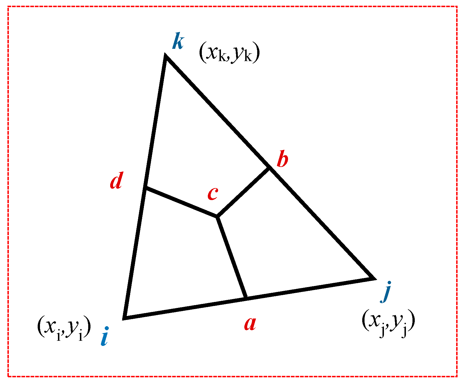
2.5. Numerical Solution

Because of the accurate description for complex boundary conditions, unstructured grid system is preferred to mesh the complex flow region of shale reservoirs, rather than Cartesian grid system. In this section, the control volume finite element method (CVFEM) based on the unstructured triangle mesh is used to obtain numerical solutions (Figure 6).
Because of the different flow and desorption mechanisms, the governing Equations (9)–(11) are distinguished. However, because the nonlinear items would be iterated by implicit solution, the matrix, fracture and hydraulic fracture systems can be expressed in a basic form.
[ λ p ] = ( ϕ / B g ) t λ = k μ B g
Equation (15) can be written in an equivalent integral form:
Ω [ λ p ] d Ω Ω ( ϕ / B g ) t d Ω = 0  
Similar to the finite difference method, the partial differential items can be written as discrete equations using CVFEM:
Ω [ λ p ] d Ω = l = 1 N T i l ( p i p l )
For the typical triangle element (Figure 7), transmissibility of CVFEM is
T i l = 1 4 A ( λ x a i a l + λ y b i b l ) ( l = j , k )
where A is the area of the triangle element, and
{ a i = y j y k ;   b i = x k x j a j = y k y i ;   b j = x i x k a k = y i y j ;   b k = x j x i
Since the partial differential of time is independent of the space domain, the discrete form of Equation (16) is
T ij ( p i p j ) + T ik ( p i p k ) A 3 Δ t ( ( ϕ B ) i n + 1 ( ϕ B ) i n ) = 0
The physical meaning of Equation (19) is the material balance in the area controlled by node i of the triangle element. For each triangle element, the balance equations of three nodes can be obtained
( T ij + T ik T ij T ik T ji T ji + T jk T jk T ki T kj T ki + T kj ) ( p i p j p k ) A 3 Δ t ( ( ϕ B ) i n + 1 ( ϕ B ) i n ( ϕ B ) j n + 1 ( ϕ B ) j n ( ϕ B ) k n + 1 ( ϕ B ) k n ) = 0
For the desorption item, it can be considered as
A 3 Δ t ( ( [ ( 1 ϕ ) V E ] ) i n + 1 ( [ ( 1 ϕ ) V E ] ) i n ( [ ( 1 ϕ ) V E ] ) j n + 1 ( [ ( 1 ϕ ) V E ] ) j n ( [ ( 1 ϕ ) V E ] ) k n + 1 ( [ ( 1 ϕ ) V E ] ) k n )
VE is the adsorbed gas volume per unit rock framework volume (m3/m3).
For the inter-porosity flux item, it can be written as
α A 3 ( ( k m / μ B g ) i 0 0 0 ( k m / μ B g ) j 0 0 0 ( k m / μ B g ) k ) ( Δ p i Δ p j Δ p k )
According to the preceding derivation, the balance equations of the systems can be expressed as:
For matrix system,
T m ( e ) p m ( e ) W ( e ) ( p m ( e ) p f ( e ) ) [ ( V E ( e ) ) n + 1 ( V E ( e ) ) n ] = [ ( N m ( e ) ) n + 1 ( N m ( e ) ) n ]
For fracture system,
T f ( e ) p f ( e ) + W ( e ) ( p m ( e ) p f ( e ) ) = [ ( N f ( e ) ) n + 1 ( N f ( e ) ) n ]
where,
η   =   m ,   f ;   p η ( e ) = ( p 1 p 2 p 3 ) η T
Tη(e) is the transmissibility matrix of element, T η ( e ) = ( T 12 k + T 13 k T 12 k T 13 k T 21 k T 21 k + T 23 k T 23 k T 31 k T 32 k T 31 k + T 32 k ) η .
Nη(e) is the cumulative matrix of element, N η ( e ) = A 3 Δ t ( ( ϕ B g ) 1 ( ϕ B g ) 2 ( ϕ B g ) 3 ) η .
W(e) is the inter-porosity flow matrix of element,
W ( e ) = α A 3 ( ( k m / μ B g ) 1 0 0 0 ( k m / μ B g ) 2 0 0 0 ( k m / μ B g ) 3 )
VE(e) is the element adsorption matrix, V E ( e ) = A 3 Δ t ( [ ( 1 ϕ t ) V E ] 1 [ ( 1 ϕ t ) V E ] 2 [ ( 1 ϕ t ) V E ] 3 ) m .
Based on discrete fracture model (Figure 8) [41,42,43], the equivalent equation for the control volume region containing discrete fractures is,
Ω d PDEs   d Ω = Ω m PDEs   d Ω m + w F × Ω f PDEs   d Ω f
Through Equation (25), the element discretization equation of fracture and hydraulic fracture system can be written,
T f + F ( e ) p f ( e ) + W ( e ) ( p m ( e ) p f ( e ) ) + Q = [ ( N f + F ( e ) ) n + 1 ( N f + F ( e ) ) n ]
where, T f + F ( e ) = η = f , F T η ( e ) and N f + F ( e ) = η = f , F N η ( e ) .

3. Results and Discussion

In this section, two representative fracture network models (discrete fracture model and dual-porosity model) are solved, and the characteristic performances of the SRV in shale are discussed. The effects of hydraulic fracture length, diffusion, Langmuir volume, fracture conductivity, stress sensitivity factor, fracture network permeability and multi-scale flow mechanisms on production performance are also analyzed. The basic synthetic data are given in Table 1.

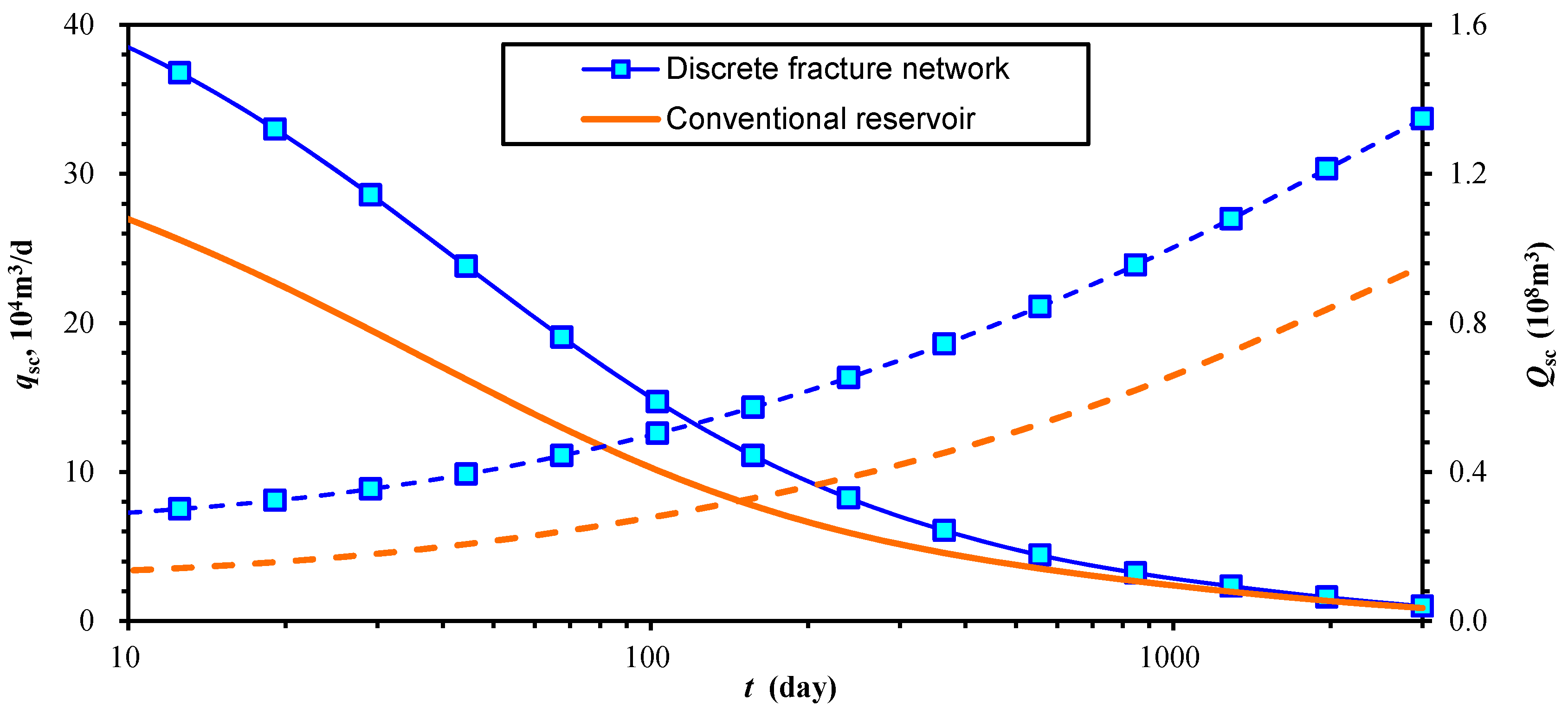
3.1. Effects of Fracture Network on Production

It is generally believed that the technique of multi-stage fractured horizontal well is the key to efficient development of shale gas reservoir. Because the fracture network system is very complex, this paper presents a discrete fracture SRV and a dual-porosity SRV system to discuss the effects of fracture network.
During hydraulic fracturing, if the net pressure for fracture extension is greater than the sum of the difference of two horizontal principle stresses and rock tensile strength, branch fractures are generated during main fracture extension, which can be described using DFN model, as shown in Figure 9.
Due to the difficulty of precisely describing the branch fractures (either geological recognition or reservoir engineering calculation), the dual-porosity composite model can be used to represent a multi-stage fractured horizontal well (MFHW) in shale gas reservoir (Figure 10).
Figure 11 compares the production rate curves of unconventional reservoirs and conventional homogeneous reservoir. At the beginning of production, high conductivity fracture network means more flow paths from reservoir to wellbore, which results in a higher production. At the latter part of production, it can be seen from the pressure distribution figures (Figure 12) that either dual-porosity model or discrete fracture model can form a large low pressure region, which improves the desorption gas production as well as reduces the flow resistance to the well.
According to the results discussion, both the dual-porosity model and the discrete fracture model can reflect the characteristic performance of SRV in shale. The contribution of fracture networks is summarized as
(1)
They improve the free gas flow capability in the early period.
(2)
They increase the flow interface between the fractured and un-fractured zone.
(3)
They stimulate the desorption of the adsorbed gas;
Notably, once the fracture distribution can be obtained quantitatively, the DFN model may present a more accurate description of the gas flow dynamic and the inter-porosity flux, especially for the early period. In the mid-later period, because the low pressure region formed by the fracture network system may hide the discreteness of fractures, the dual-porosity model would obtain the satisfied results. Although the DFN model needs more complicated treatments and calculations than the dual-porosity model, limited by uncertainty of the fracture network, the dual-porosity model is still a useful and recommended method for numerical simulation in shale. In view of this, the dual-porosity model is used to analyze the sensitivity in the next section.

3.2. Sensitivity Analyses

Different from conventional reservoirs, gas flow in shale is affected by many characteristic parameters, such as hydraulic fracture numbers, hydraulic fracture length, hydraulic fracture height, conductivity Langmuir volume and stress sensitivity factor.

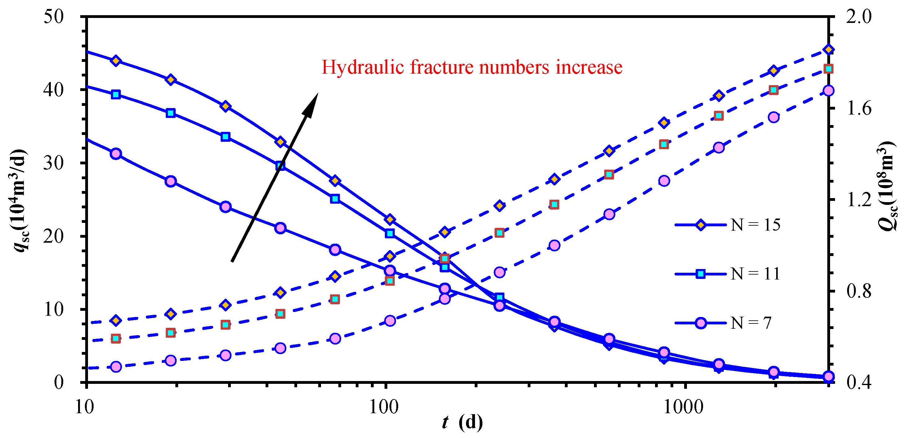
3.2.1. Hydraulic Fracture Numbers (N)

Figure 13 shows the influence of hydraulic fracture number on production performance of the horizontal well. With the increase of hydraulic fracture numbers, gas production increases; such effect becomes smaller with increase of the fracture numbers. For the same fracture and horizontal well length, there is an optimal number for hydraulic fractures. At the late production period, flow will form an approximately rectangular area of low pressure, which can be considered as a potential body. Thus, the effect of number of fractures on the production becomes very small. After 500 days, the production rates of horizontal wells with different numbers of fractures are almost equal, and, according to the material balance principle, cumulative production of each well is close to the same after a long time.

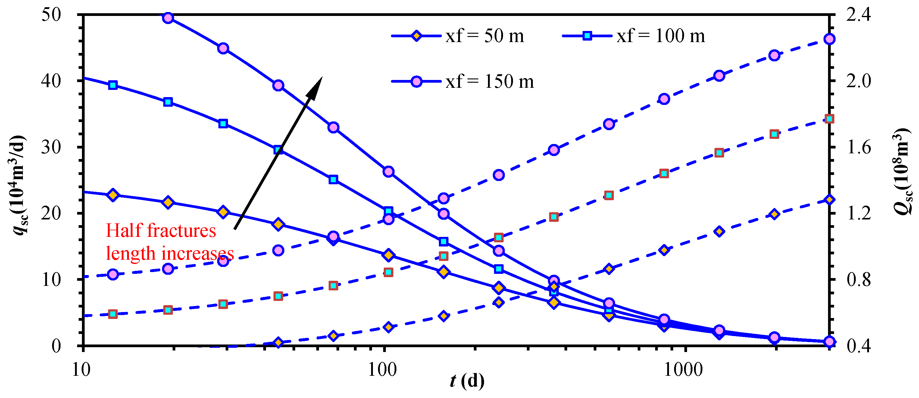
3.2.2. Hydraulic Fracture Length (xF)

Figure 14 shows the effect of the fracture length on the production of a MFH well in shale reservoir. As the fracture length increases, production rate and cumulative production increase. This is because the fracture half-length increase will significantly improve the single well controlling area with the same horizontal well length. The figure shows the production performance of a MFH well with fracture half-length of 50 m, 100 m and 150 m, corresponding, respectively, to model regions 1200 m × 300 m, 1200 m × 400 m and 1200 m × 500 m. Therefore, in the development of shale gas reservoir, extension of the fracture length can obtain higher production.

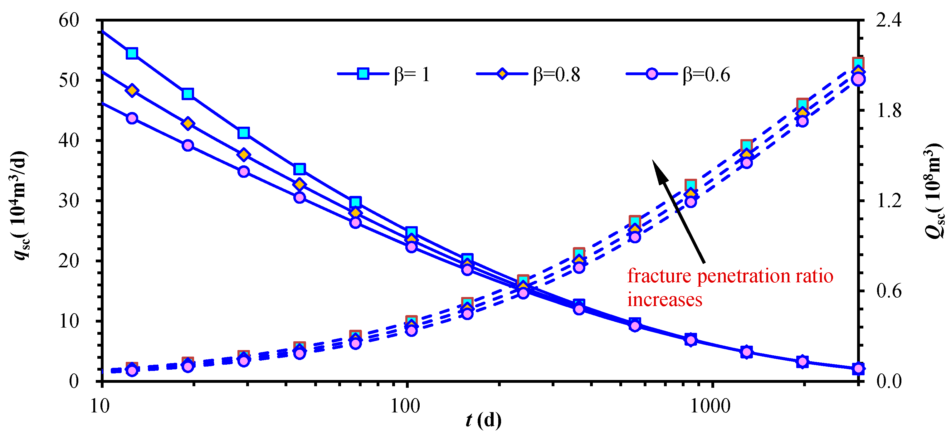
3.2.3. Hydraulic Fracture Height (hF)

The fracture penetration ratio β, which is the ratio of hydraulic fracture height to reservoir thickness, is defined as
β = h F h
Figure 15 shows the influence of hydraulic fracturing degree on production of a MFH well in shale gas reservoir. Fracture penetration ratio directly affects the early production. After some days, an approximate rectangular low pressure region is created surrounding the multistage fractured horizontal well. At this time, the effect of fracture penetration ratio is not obvious.

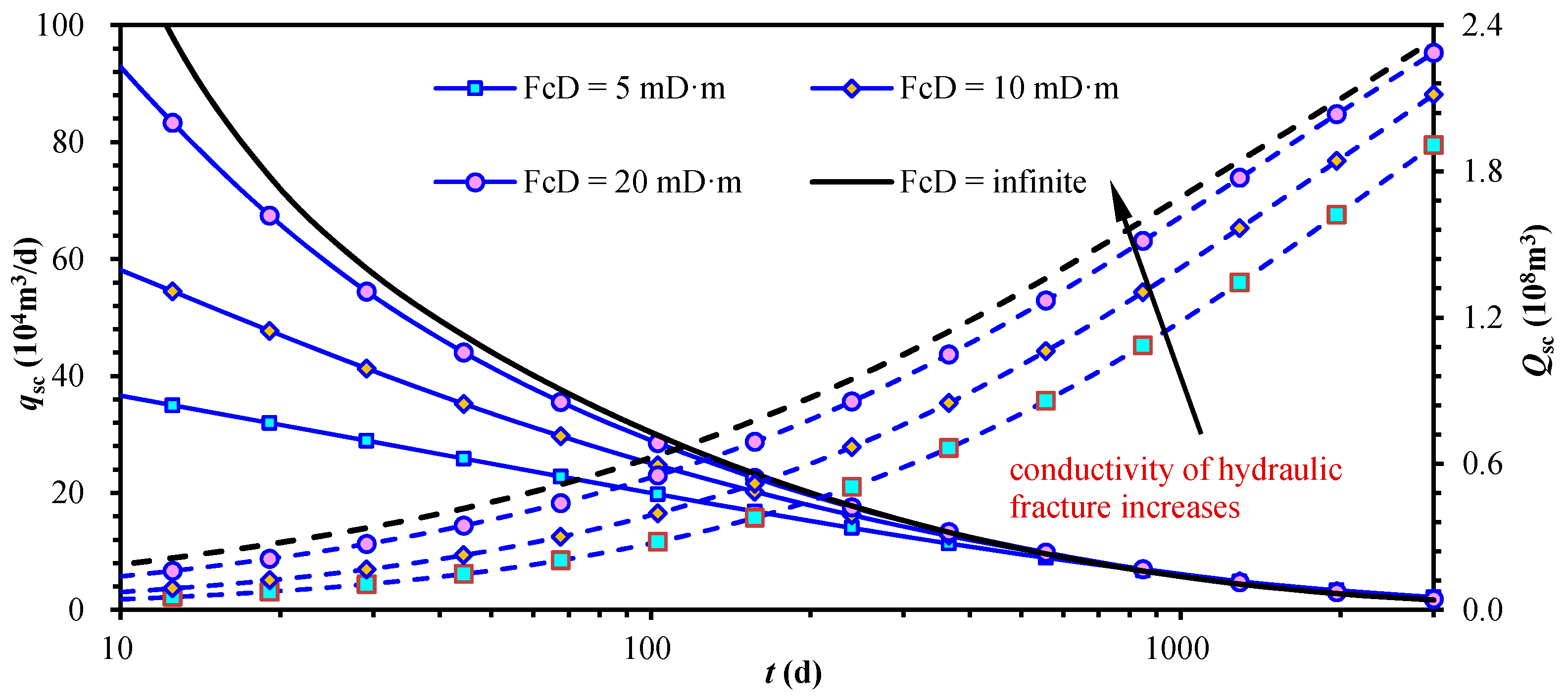
3.2.4. Hydraulic Fracture Conductivity (FcD)

The effect of hydraulic fracture conductivity on production is shown in Figure 16. It can be seen that production rate and cumulative production of the fractured horizontal well increase with increase of fracture conductivity. This effect is more obvious during the early-time flow period and diminishes with production time. Note that the increase of early production with fracture conductivity tends to maximize at certain level. As shown in the plot, for hydraulic fracture conductivity of 20 mD·m, the production rate and cumulative production are close to those of a horizontal well with infinite conductive fractures.
According to previous analysis, there is an optimal value of fracture conductivity for hydraulic fracturing design. For fracture conductivity of 20 mD·m, the calculated fracture permeability is 20D for fracture width of 0.001 m. Obviously, this is easy to achieve during normal fracturing operation. Therefore, it is not worth trying to improve well production through increasing hydraulic fracture conductivity.

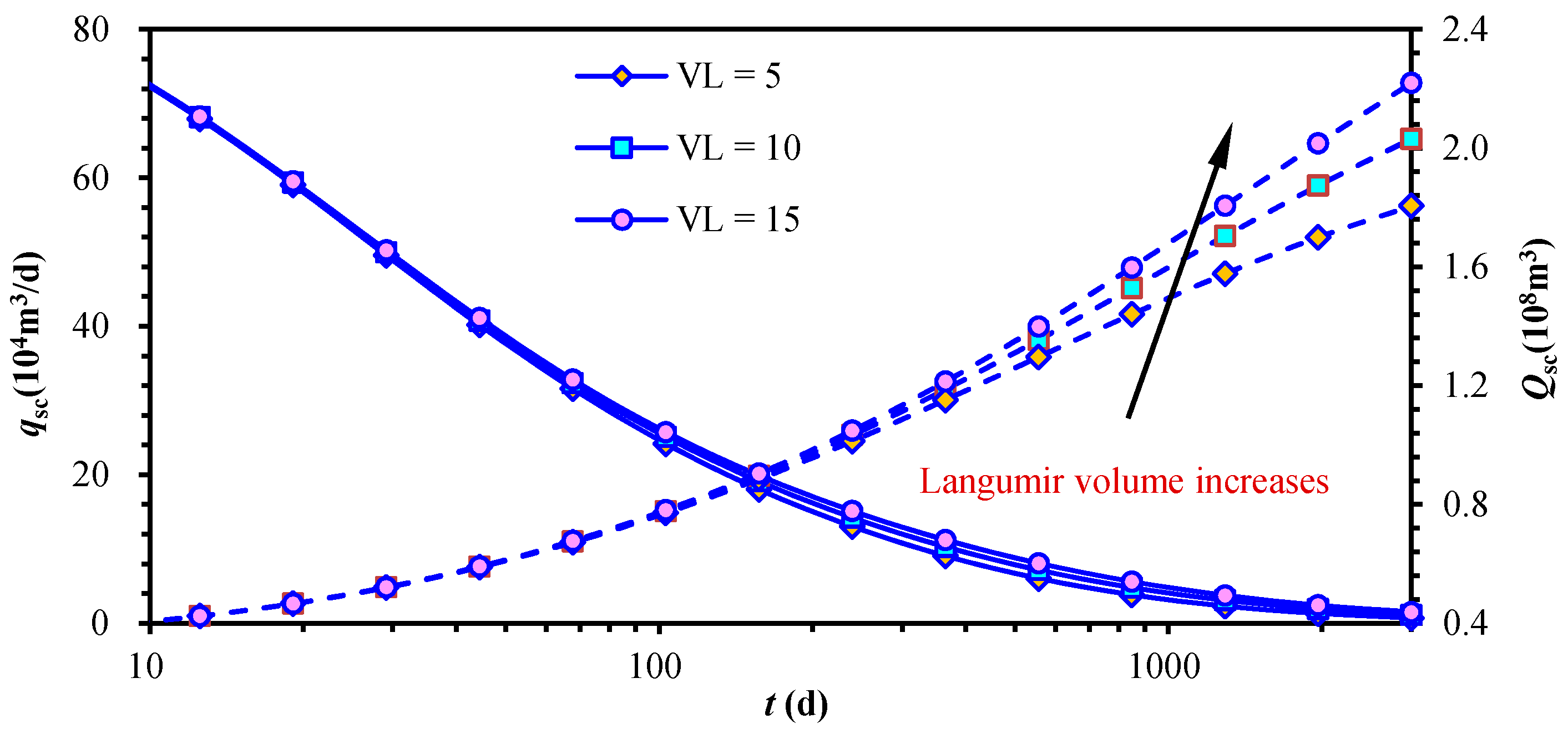
3.2.5. Langmuir Volume (Vm)

The influences of Langmuir volume on production performance is shown in Figure 17. It is clearly observed that VL mainly influences the curves in the mid-later flow period, which is the inter-porosity flow between matrix and natural fracture system. The larger VL is, the greater production rate for a constant BHP; after the quick decline period, production curve becomes flat. This is because a bigger value of Langmuir volume represents a larger amount of adsorbed gas in shale matrix which decreases the formation pressure drop and supplements the gas capacity.

3.2.6. Stress Sensitivity Coefficient (α)

As Figure 18 shows, the production rate and accumulative production both decrease when stress sensitivity increases. According to Equation (14), when pressure declines, the higher stress sensitivity leads to higher decrease of natural fracture permeability. If we assume the stress sensitivity coefficient is 0.01, 0.05 and 0.1, after 3000 days, the recovery is 52%, 49% and 47%, respectively.

4. Conclusions

This paper focuses on the flow rate performance of a MFH well in shale. Based on the discrete fracture model and dual-porosity model, the influences of fracture network system is analyzed. Moreover, with the consideration of gas adsorption/desorption, stress dependence and multi-scale flow mechanisms in the equations, the sensitivities of the characteristic parameters in shale are discussed. The main conclusions of this paper can be summarized as follows:
(1)
The contribution of fracture networks on productivities can be described as:
(a)
They improve the free gas flow capability in the early period.
(b)
They increase the flow interface between the fractured and un-fractured zone.
(c)
They stimulate the desorption of the adsorbed gas.
(2)
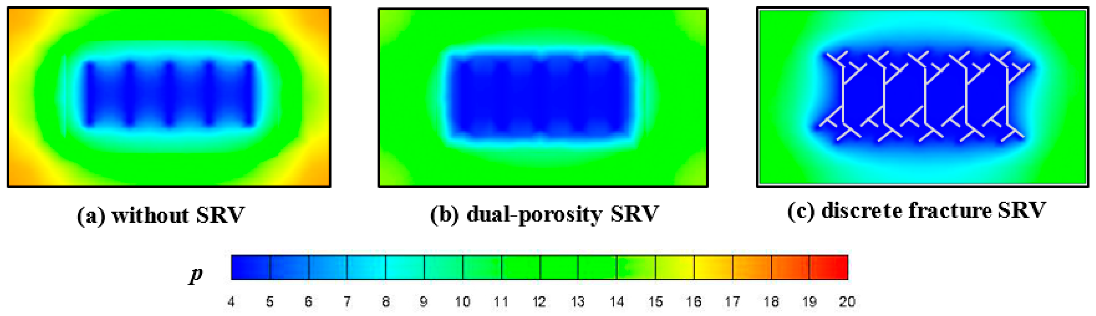
Once the fracture distribution can be obtained quantitatively, the DFN model may present a more accurate description of the gas flow dynamic and the inter-porosity flux in the early flow period. Nevertheless, limited by uncertainty of the fracture network, the dual-porosity model is still a useful and recommended method for numerical simulation in shale.
(3)
Sensitivity analyses reveal that the increases of hydraulic fracture number, length and Langmuir volume represent a higher flow rate, and the marginal effect of fractures number should be noticed in fracturing engineering.

Acknowledgments

This work is supported by the National Natural Science Foundation of China (Grant No. 51534006).

Author Contributions

Yu Dai analyzed the experiment data; Xinhua Ma provided core samples and designed the study; Liehui Zhang corrected English; Bing Zhong deduced formulas; Jianfa Wu drawn figures; Zhengwu Tao searched literatures; Deliang Zhang wrote the paper.

Conflicts of Interest

The authors declare no conflict of interest.

Nomenclature

Bgthe ratio of gas volume at reservoir condition and gas volume at surface condition, rm3/sm3
hformation thickness, m
KnKnudsen number, dimensionless
kBBoltzmann constant, kB = 1.3806 × 10⁻²³ J/K
kpermeability, mD
Lcharacteristic length of shale pore, nm
Mggas molecular weight, g/mol
pLLangmuir pressure, MPa
Rgas constant, 8.314 J/(mol·K)
Ttemperature, K
VLLangmuir volume, sm3/m3
VEadsorbed gas volume per unit rock volume at a constant pressure, sm3/m3
Zthe ratio of real gas volume and ideal gas volume, m3/m3
λgas molecular mean free path, nm
δmolecule collision distance, nm
μgas viscosity, mPa·s
ϕporosity, fraction
Subscript
mmatrix
ffracture
Fhydraulic fracture

References

  1. Wang, K.; Liu, H.; Luo, J.; Wu, K.; Chen, Z. A comprehensive model coupling embedded discrete fractures, multiple interacting continua and geomechanics in shale gas reservoirs with multi-scale fractures. Energy Fuel 2017, 31, 7758–7776. [Google Scholar] [CrossRef]
  2. Wu, K.; Li, X.; Wang, C.; Yu, W.; Chen, Z. Model for surface diffusion of adsorbed gas in nanopores of shale reservoirs. Ind. Eng. Chem. Res. 2015, 54, 3225–3236. [Google Scholar] [CrossRef]
  3. Chen, Z.; Huan, G.; Ma, Y. Computational Methods for Multiphase Flows in Porous Media; Society for Industrial and Applied Mathematics: Philadelphia, PA, USA, 2006. [Google Scholar]
  4. Bustin, R.M.; Bustin, A.M.; Cui, A.; Ross, D.; Pathi, V.M. Impact of shale properties on pore structure and storage characteristics. In Proceedings of the SPE Shale Gas Production Conference, Fort Worth, TX, USA, 16–18 November 2008. [Google Scholar]
  5. Jenkins, C.D.; Boyer, C.M. Coalbed- and shale-gas reservoirs. J. Pet. Technol. 2008, 60, 92–97. [Google Scholar] [CrossRef]
  6. Curtis, B.J. Fractured shale-gas systems. AAPG Bull. 2002, 86, 1921–1938. [Google Scholar]
  7. Wu, Y.S.; Li, J.; Ding, D.; Wang, C.; Di, Y. A generalized framework model for the simulation of gas production in unconventional gas reservoirs. SPE J. 2014, 19, 845–857. [Google Scholar] [CrossRef]
  8. Hill, D.G.; Nelson, C.R. Gas Productive Fractured Shales: An Overview and Update. Gas TIPS 2000, 6, 4–13. [Google Scholar]
  9. Mengal, S.A.; Wattenbarger, R.A. Accounting for adsorbed gas in shale gas reservoirs. In Proceedings of the SPE Middle East Oil and Gas Show and Conference, Manama, Bahrain, 25–28 September 2011. [Google Scholar]
  10. Zhang, Z.Y.; Yang, S.B. On the adsorption and desorption trend of shale gas. J. Exp. Mech. 2012, 27, 492–497. (In Chinese) [Google Scholar]
  11. Alnoaimi, K.R.; Kovscek, A.R. Experimental and numerical analysis of gas transport in shale including the role of sorption. In Proceedings of the SPE Annual Technical Conference and Exhibition, New Orleans, LA, USA, 30 September–2 October 2013. [Google Scholar]
  12. Yu, W.; Sepehrnoori, K.; Patzek, T.W. Evaluation of gas adsorption in Marcellus Shale. In Proceedings of the SPE Annual Technical Conference and Exhibition, Amsterdam, The Netherlands, 27–29 October 2014. [Google Scholar]
  13. Lu, X.C.; Li, F.C.; Watson, A.T. Adsorption studies of natural gas storage in Devonian Shales. SPE Form. Eval. 1995, 10, 109–113. [Google Scholar] [CrossRef]
  14. Shabro, V.; Torres-Verdin, C.; Sepehrnoori, K. Forecasting gas production in organic shale with the combined numerical simulation of gas diffusion in Kerogen, Langmuir desorption from surfaces, and advection in nanopores. In Proceedings of the 2012 SPE Annual Technical Conference and Exhibition, San Antonio, TX, USA, 8–10 October 2012. [Google Scholar]
  15. Dong, Z.; Holditch, S.A.; Mcvay, D.A. Resource evaluation for shale gas reservoirs. In Proceedings of the SPE Hydraulic Fracturing Technology Conference, The Woodlands, TX, USA, 6–8 February 2012. [Google Scholar]
  16. Haghshenas, B.; Clarkson, C.R.; Chen, S. Multi-porosity multi-permeability models for shale gas reservoirs. In Proceedings of the SPE Unconventional Resources Conference Canada, Calgary, AB, Canada, 5–7 November 2013. [Google Scholar]
  17. Ertekin, T.; King, G.R.; Schwerer, F.C. Dynamic gas slippage: A unique dual-mechanism approach to the flow of gas in tight formations. SPE Form. Eval. 1986, 1, 43–52. [Google Scholar] [CrossRef]
  18. Roy, S.; Raju, R. Modeling gas flow through micro channels and nanopores. J. Appl. Phys. 2003, 93, 4870–4878. [Google Scholar] [CrossRef]
  19. Ozkan, E.; Raghavan, R.; Apaydin, O.G. Modeling of fluid transfer from shale matrix to fracture network. In Proceedings of the SPE Annual Technical Conference and Exhibition, Florence, Italy, 20–22 September 2010. [Google Scholar]
  20. Javadpour, F.; Fisher, D.; Unsworth, M. Nanoscale gas flow in shale gas sediments. J. Gas Can. Pet. Technol. 2007, 46, 55–61. [Google Scholar] [CrossRef]
  21. Javadpour, F. Nanopores and apparent permeability of gas flow in mudrocks (shales and siltstone). J. Gas Can. Pet. Technol. 2009, 48, 16–21. [Google Scholar] [CrossRef]
  22. Javadpour, F.; Moghanloo, G.R. Contribution of Methane Molecular Diffusion in Kerogen to Gas-in-Place and Production. In Proceedings of the SPE Western Regional & AAPG Pacific Section Meeting 2013 Joint Technical Conference, Monterey, CA, USA, 19–25 April 2013. [Google Scholar]
  23. Civan, F. Effective correlation of apparent gas permeability in tight porous media. Trans. Porous Media 2010, 82, 375–384. [Google Scholar] [CrossRef]
  24. Civan, F.; Rai, C.S.; Sondergeld, C.H. Shale-gas permeability and diffusivity inferred by improved formulation of relevant retention and transport mechanisms. Trans. Porous Media 2011, 86, 925–944. [Google Scholar] [CrossRef]
  25. Civan, F.; Devegowda, D.; Sigal, R. Critical evaluation and improvement of methods for determination of matrix permeability of shale. In Proceedings of the SPE Annual Technical Conference and Exhibition, New Orleans, LA, USA, 30 September–2 October 2013. [Google Scholar]
  26. Swami, V.; Settari, A. A pore scale gas flow model for shale gas reservoir. In Proceedings of the Americas Unconventional Resources Conference, Pittsburgh, PA, USA, 5–7 June 2012. [Google Scholar]
  27. Deng, J.; Zhu, W.Y.; Ma, Q. A new seepage model for shale gas reservoir and productivity analysis of fractured well. Fuel 2014, 124, 232–240. [Google Scholar] [CrossRef]
  28. Wu, Y.S.; Moridis, G.J.; Bai, B.; Zhang, K. A Multi-Continuum Model for Gas Production in Tight Fractured Reservoirs. In Proceedings of the SPE Hydraulic Fracturing Technology Conference, The Woodlands, TX, USA, 19–21 January 2009. [Google Scholar]
  29. Bello, R.O.; Watenbargen, R.A. Multi-stage hydraulically fractured horizontal shale gas well rate transient analysis. In Proceedings of the 2010 SPE North Africa Technical Conference and Exhibition-Energy Management in a Challenging Economy, Cairo, Egypt, 14–17 February 2010. [Google Scholar]
  30. Aboaba, A.; Cheng, Y. Estimation of fracture properties for a horizontal well with multiple hydraulic fractures in gas shale. In Proceedings of the 2010 SPE Eastern Regional Meeting, Morgantown, WV, USA, 13–15 October 2010. [Google Scholar]
  31. Ozkan, E.; Brown, M.; Raghavan, R.; Kazemi, H. Comparison of fractured-horizontal-well performance in tight sand and shale reservoirs. SPE Reserv. Eval. Eng. 2011, 14, 248–259. [Google Scholar] [CrossRef]
  32. Brown, M.; Ozkan, E.; Ragahavan, R.; Kazemi, H. Practical solutions for pressure-transient responses of fractured horizontal wells in unconventional shale reservoirs. SPE Reserv. Eval. Eng. 2011, 14, 663–676. [Google Scholar] [CrossRef]
  33. Stalgorova, E.; Mattar, L. Practical analytical model to simulate production of horizontal wells with branch fractures. In Proceedings of the SPE Canadian Unconventional Resources Conference, Calgray, AB, Canada, 30 October–1 November 2012. [Google Scholar]
  34. Jiang, J.M.; Rami, M.Y. A multimechanistic multicontinuum model for simulating shale gas reservoir with complex fractured system. Fuel 2015, 161, 333–344. [Google Scholar] [CrossRef]
  35. Wang, J.; Luo, H.; Liu, H.; Ji, Y.; Cao, F.; Li, Z.; Sepehrnoori, K. Variations of Gas Flow Regimes and Petro-Physical Properties During Gas Production Considering Volume Consumed by Adsorbed Gas and Stress Dependence Effect in Shale Gas Reservoirs. In Proceedings of the 2015 SPE Annual Technical Conference & Exhibition, Houston, TX, USA, 28–30 September 2015. [Google Scholar]
  36. Wang, F.P.; Reed, R.M. Pore networks and fluid flow in gas shales. In Proceedings of the 2009 SPE Annual Technical Conference & Exhibition, New Orleans, LA, USA, 4–7 October 2009. [Google Scholar]
  37. Silin, D.; Kneafsey, T. Shale gas: Nanometer-scale observations and well modelling. J. Can. Pet. Technol. 2012, 51, 464–475. [Google Scholar] [CrossRef]
  38. Zhao, Y.L.; Zhang, L.H.; Zhao, J.Z.; Luo, J.X.; Zhang, B.N. Triple porosity modeling of transient well test and rate decline analysis for multi-fractured horizontal well in shale gas reservoirs. J. Pet. Sci. Eng. 2013, 110, 253–262. [Google Scholar] [CrossRef]
  39. Wang, H.T. Performance of multiple fractured horizontal wells in shale gas reservoirs with consideration of multiple mechanisms. J. Hydrol. 2014, 510, 299–312. [Google Scholar] [CrossRef]
  40. Computer Modeling Group Ltd. (CMG). GEM User Guide; Computer Modeling Group Ltd.: Calgary, AB, Canada, 2012. [Google Scholar]
  41. Karimi-Fard, M.; Firoozabadi, A. Numerical simulation of water injection in 2D fractured media using discrete-fracture network. In Proceedings of the 2001 SPE Annual Technical Conference & Exhibition, New Orleans, LA, USA, 30 September–3 October 2001. [Google Scholar]
  42. Karimi-Fard, M.; Durlofsky, L.J.; Aziz, K. An Efficient Discrete-Fracture Model Applicable for General-Purpose Reservoir Simulators. In Proceedings of the 2003 SPE Reservoir Simulation Symposium, Houston, TX, USA, 3–5 February 2003. [Google Scholar]
  43. Moinfar, A.; Varavei, A.; Sepehrnoori, K.; Johns, R.T. Development of a coupled dual continuum and discrete fracture model for the simulation of unconventional reservoirs. In Proceedings of the 2013 SPE Reservoir Simulation Symposium, The Woodlands, TX, USA, 18–20 February 2013. [Google Scholar]
Figure 1. The flow in nan-pores of shale reservoirs.
Energies 11 00414 g001
Figure 2. Hydraulic multiple fractured horizontal well with the stimulated reservoir volume (SRV) and its simplified models.
Energies 11 00414 g002
Figure 3. Gas storage and flow mechanisms in shale gas reservoirs.
Energies 11 00414 g003
Figure 4. The pore distributions curves of Longmaxi formation Sichuan basin.
Energies 11 00414 g004
Figure 5. The Knudsen number of different pore diameters.
Energies 11 00414 g005
Figure 6. The triangle meshes and control volume.
Energies 11 00414 g006
Figure 7. The typical triangle element.
Energies 11 00414 g007
Figure 8. Concise description of the discrete fracture model network (DFN) model.
Energies 11 00414 g008
Figure 9. DFN model mesh of a fracture network system in shale.
Energies 11 00414 g009
Figure 10. Dual-porosity model of a fracture network system in shale.
Energies 11 00414 g010
Figure 11. Curves of production rate and accumulative production of a multi-stage fractured horizontal well (MFHW) in shale.
Energies 11 00414 g011
Figure 12. The pressure distributions of different SRV models (3000 days).
Energies 11 00414 g012
Figure 13. Effect of hydraulic fracture numbers increase on production of a MFHW in shale.
Energies 11 00414 g013
Figure 14. Effect of the fracture length on the production of shale gas reservoirs.
Energies 11 00414 g014
Figure 15. Effect of Hydraulic Fracturing Degree on Production of a MFHW in Shale.
Energies 11 00414 g015
Figure 16. Effect of Hydraulic Fracture Conductivity on Production of a MFHW in Shale.
Energies 11 00414 g016
Figure 17. Effect of Langmuir volume on production performance of a MFHW in shale.
Energies 11 00414 g017
Figure 18. Effect of stress sensitivity coefficient on production performance of a MFHW in shale.
Energies 11 00414 g018
Table 1. Synthetic data used for the results discussion.
Reservoir ParametersValueReservoir ParametersValue
Formation thickness, h, m50Reservoir boundary, X × Y, m800 × 500
Initial reservoir pressure, pi, MPa 20Reservoir temperature, T, °C100
Gas specific gravity, rg, fraction0.6Bottom-hole pressure, pw, MPa4
Horizontal wellbore length, L, m1000Hydraulic fractures numbers, N5
Half fracture length, xf, m100Langmuir pressure, PL, MPa4
Inner region fracture porosity, Φf1, %3Inner region fracture permeability, kf1, mD0.01
Outer region fracture porosity, Φf2, %1Outer region fracture permeability, kf2, mD0.001
Matrix porosity, Φm, %1Matrix permeability, km, mD0.0001
Hydraulic fracture width, m0.001Stress sensitive coefficient, α, MPa−10.01
Langmuir Volume, VL, m3/m310--

