Article

Hypothesis Tests-Based Analysis for Anomaly Detection in Photovoltaic Systems in the Absence of Environmental Parameters

Department of Electrical and Information Engineering, Polytechnic University of Bari, st. E. Orabona 4, I-70125 Bari, Italy
Energies 2018, 11(3), 485; https://doi.org/10.3390/en11030485
Submission received: 28 January 2018 / Revised: 18 February 2018 / Accepted: 22 February 2018 / Published: 25 February 2018
(This article belongs to the Special Issue PV System Design and Performance)

Abstract

:
This paper deals with the monitoring of the performance of a photovoltaic plant, without using the environmental parameters such as the solar radiation and the temperature. The main idea is to statistically compare the energy performances of the arrays constituting the PV plant. In fact, the environmental conditions affect equally all the arrays of a small-medium-size PV plant, because the extension of the plant is limited, so any comparison between the energy distributions of identical arrays is independent of the solar radiation and the cell temperature, making the proposed methodology very effective for PV plants not equipped with a weather station, as it often happens for the PV plants located in urban contexts and having a nominal peak power in the 3÷50 kWp range, typically installed on the roof of a residential or industrial building. In this case, the costs of an advanced monitoring system based on the environmental data are not justified, consequently, the weather station is often also omitted. The proposed procedure guides the user through several inferential statistical tools that allow verifying whether the arrays have produced the same amount of energy or, alternatively, which is the worst array. The procedure is effective in detecting and locating abnormal operating conditions, before they become failures.

1. Introduction

The random variability of atmospheric phenomena affects the available irradiance intensity for photovoltaic (PV) generators. During the clear days an analytic expression for the solar irradiance can be defined, whereas this is not possible for cloudy days. The effects of the environmental conditions are studied in [1,2,3,4,5]. After the installation of a PV plant, a system for monitoring the energy performance in every environmental condition is needed. As the modules are main components of a PV plant, deep attention is focused on their state of health [6]. For this reason, techniques commonly used to verify the presence of typical defects in PV modules are based on infrared analysis [7,8], eventually supported by unmanned aerial vehicles [9], on luminescence imaging [10], or on their combination [11], while automatic procedures to extract information using thermograms are proposed in [12,13]. Nevertheless, these approaches regard single modules of the PV plants. When there is no information about the general operation of the PV plant, other techniques can be considered to prevent failures and to enhance the energy performance of the PV system, such as artificial neural networks [3,14], statistics [15,16,17], and checking the electrical variables [18,19,20]. More in detail, some of the PV fault detection algorithms are based on electrical circuit simulation of the PV generator [21,22], while other researchers use approaches based on the electrical signals [23,24]. Moreover, predictive model approaches for PV system power production based on the comparison between measured and modeled PV system outputs are discussed in [15,25,26,27]. Standard benchmarks [28], called final PV system yield, reference yield and Performance Ratio (PR), are currently used to assess the overall system performance in terms of energy production, solar resource, and system losses. These benchmarks have been recently used to review the energy performance of 993 residential PV systems in Belgium [29] and 6868 PV installations in France [30]. Unfortunately, these indices have two drawbacks: they only supply rough information about the performance of the overall PV plant and they do not allow any assessment of the behavior of single PV plant parts. Moreover, when important faults such as short circuits or islanding occur, the electrical variables and the produced energy have fast and not negligible variations, so they are easily detected. These events produce drastic changes and can be classified as high-intensity anomalies. On the other hand, low-intensity anomalies such as the ageing of the components or minimal partial shading produce minimal variations on the electrical variables and on the produced energy, so they are not easily detectable. Moreover, these minor anomalies can evolve into failures or faults, so their timely identification can avoid more serious failures and limit the occurrence of out of order states. With respect to the configuration defined in the design stage, any PV plant can be single-array or multi-array, being an array a set of connected PV modules, for which the electrical variables and the produced energy are measured. Moreover, PV plants with only two arrays are not common: the alternatives are between one-array PV plant—this is the case of small nominal peak power PV plant—and multiple-array PV plant for higher nominal peak power PV plant. The multiple-array solution is very common, because it has several advantages, thanks to the partition of the produced energy: lower current for each array (thus reduced section of the solar cables), high flexibility in the choice of the components (inverter, switches, electrical boxes, etc.), O&M services on each single array, avoiding situations where the whole plant is out of order, and so on. Moreover, the large PV plants, having a nominal peak power higher than 100 kWp are usually equipped with a weather station, able to measure and store the environmental parameters, which affect the energy production, i.e., the solar irradiance, temperature and wind. Frequently, the large PV plants with nominal peak power higher than 1 MWp are equipped with more than one weather station, because of the large occupied area, typically about 2 ha/MWp. Obviously, these last ones are solar farms and are located in extra-urban territory. Instead, the PV plants usually installed in a urban context have a nominal peak power that ranges between 3÷50 kWp; the minimum value refers, for example, to a PV plant on the roof of a residential building, while the maximum value corresponds to a PV plant of a small company that locates it on the roof of its industrial building or in a free private area. These PV plants are usually multi-array and are not equipped with a weather station, because the costs of an advanced monitoring system are not negligible with respect to the initial investment as well as to the costs of a yearly O&M service, so these medium size PV plants are usually equipped with a simplified monitoring system, which stores the total produced energy, the electrical variables on the AC and DC side, having also the possibility to send alerts to the owner via SMS or email. This system does not perform any analysis of the produced energy, so it cannot detect any anomaly before it becomes a failure, and it can only alert when the failure is already happened. In these cases, valid support is provided by the PhotoVoltaic Geographical Information System (PVGIS) [31] of the European Commission Joint Research Centre (EC-JRC) that is based on the historical data of the solar irradiance. 
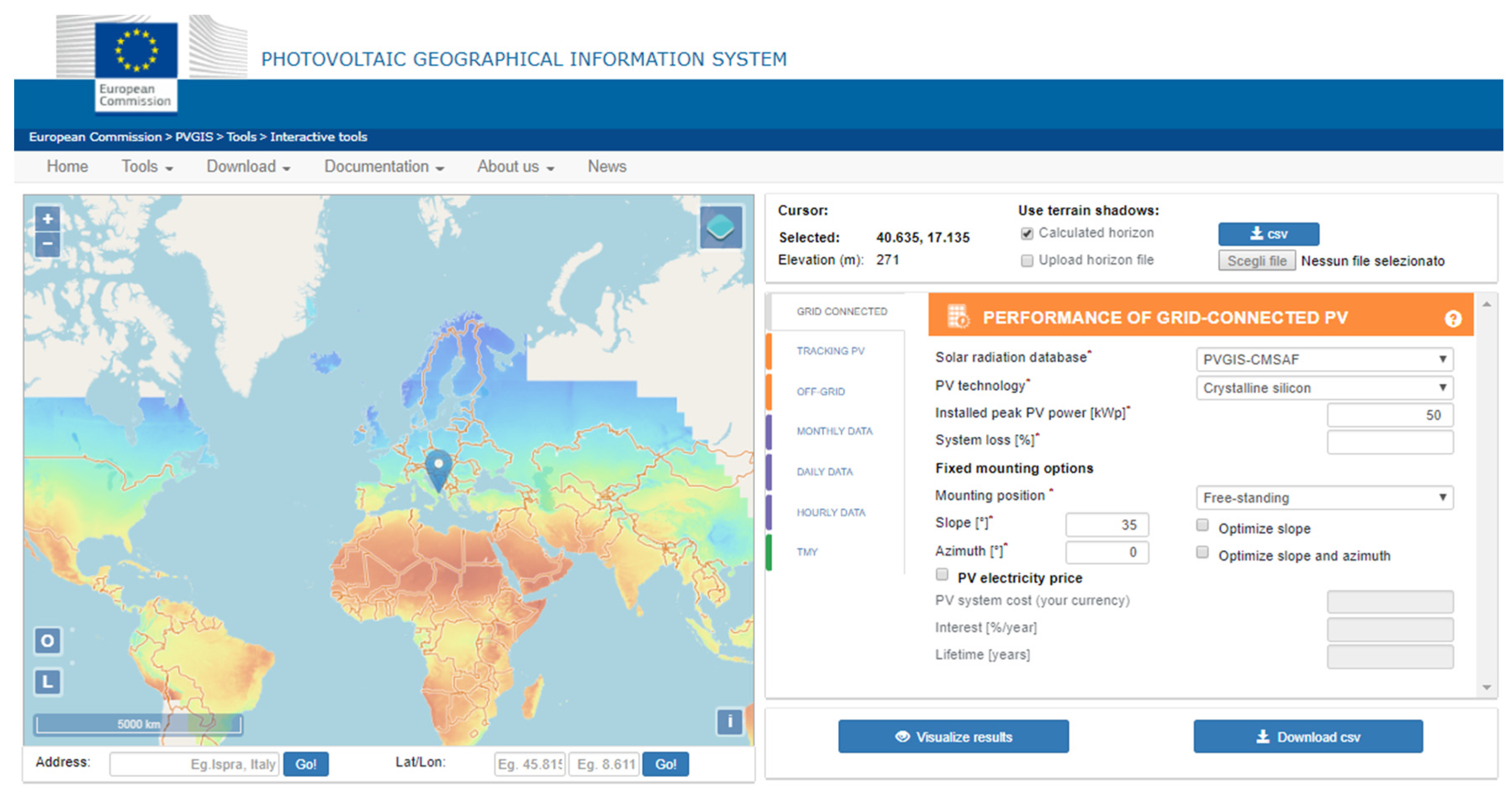
Figure 1 is a screenshot of the website. On the left hand-side, a colored map with the solar radiation is reported and the user can select the location of the PV plant, whereas, on the right hand-side, the user can insert the information on the typology of the PV plant (off-grid, grid-connected, tracking-based), the specifications of the PV plant (module technology, slope, rated power, etc.), and the required energy production data (monthly, daily, hourly). In this way, it is possible to estimate the productivity of the PV plant under investigation and to compare it with the real energy production. This can represent a preliminary check of the operation of the PV plant and will be used later, in the Section 3 and Section 4. Nevertheless, it is extremely important to prevent a failure, detecting any anomaly in a timely way for two reasons. Firstly, when an anomaly is present, the energy production is already lower than the expected one and this implies an economic loss. Secondly, a timely action of the O&M service allows restoring the damaged parts of the PV systems with minimum costs and minimum time out of order, reducing either the Mean Time To Repair (MTTR)—because the damage is limited—or the Mean Down Time (MDT), because the restore action is planned while the PV plant is still operating. This strategy, evidently, greatly increases the availability of the PV plant and its yearly energy performance.
With this in mind, this paper proposes a methodology to detect an anomaly in the operation of a PV system; this methodology can be easily applied to any multi-array PV plant, but it is particularly useful for PV plants not equipped with a weather station. This is often the situation of the PV plants in urban contexts, as previously explained. The proposed methodology, in fact, compares the energy distributions of the arrays with each other, on the basis of a statistical algorithm that does not consider the environmental parameters as inputs. This is possible because the area occupied by the PV modules of a PV plant in the urban context is limited and then the average environmental conditions can be considered to affect the identical arrays in the same way. The proposed procedure is completely based on several hypothesis tests and is a cheap and fast approach to monitor the energy performance of a PV system, because no additional hardware is required. The procedure also allows continuous monitoring because it is cumulative and new data can be added to the initial dataset, as they are acquired by the measurement system. The methodology is based on an algorithm, which suggests the user, step by step, the suitable statistical tool to use. The first one is the Hartigan’s Dip Test (HDT) that is able to discriminate an unimodal distribution from a multimodal one. The verification of the unimodality can be also done on the basis of a relationship between the values of skewness and kurtosis [32,33]; nevertheless, in this paper only HDT will be used, because it is usually more sensitive than other methods. The check on the unimodality is very important to decide whether a parametric test can be used to compare the energy distributions of the arrays or not, because the parametric tests, being based on known distributions, are more performing than the nonparametric ones. Nevertheless, the parametric tests can be applied, only if specific assumptions are satisfied. A powerful parametric test to compare more than two statistical distributions is the well-known ANalysis Of VAriance (ANOVA) [34] that is based on three assumptions. The proposed algorithm suggests using the Jarque-Bera’s test and the Bartlett’s test to verify the assumptions. In the negative case, the procedure suggests to use the Kruskal-Wallis test or the Mood’s median test, in absence or in presence of outliers in the dataset, respectively. As a last step, Tukey’s test is run to do a multi-comparison one-by-one between the mean values of the distributions, in order to determine which estimates are significantly different.
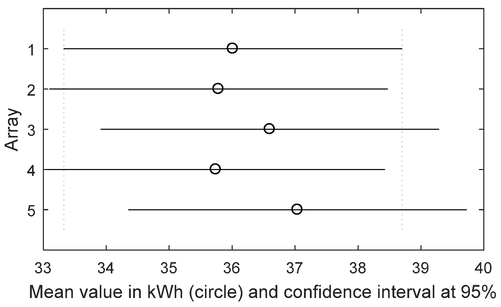
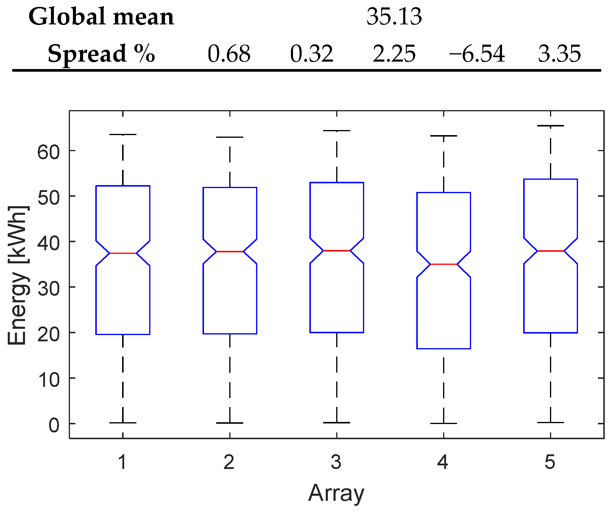
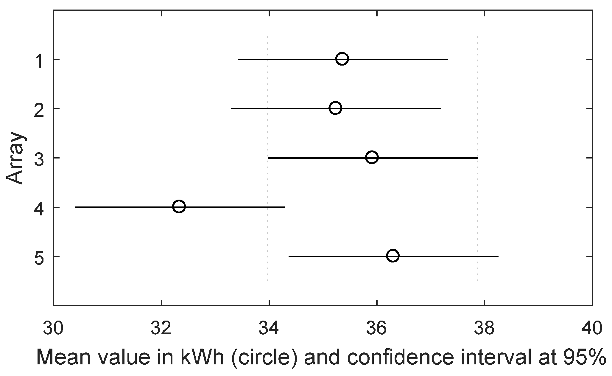
A case-study is discussed in the paper. The algorithm is applied to a real operating PV plant and the methodology is run four times: the first one, based on the energy dataset of one month; the second one, based on the energy dataset of three months; the third one, based on the energy dataset of six months; the last one, based on the energy dataset of the whole year. The paper is structured as follows: Section 2 describes the proposed algorithm, Section 3 describes the PV system under examination, Section 4 discusses the results, and the Conclusions end the paper.

2. Statistical Methodology

In this paper, it is consider that the PV plant is composed of A identical arrays, with A > 2 for the reasons already explained in the Introduction. This constraint is mandatory for the proposed methodology, because it is based on the comparison among the energy distributions of the arrays constituting the PV system. Each array is usually equipped with a measurement system that measures the values of the produced energy in AC, other than the values of voltage and current of both the DC and AC sides of the inverter, with a fixed sampling time, ∆t. At the generic time-instant t = qt of the j-th day, the q-th sample vector of the k-th array is defined as x j , k ( q ) = [ E j , k ( q )   v j , k , D C ( q )   i j , k , D C ( q )   v j , k , A C ( q )   i j , k , A C ( q ) ] , for k = 1 , , A , j = 1 , , D (being D the number of the investigated days), q = 1 , , Q , where q = 1 characterizes the first daily sample at the analysis time t = Δ t and q = Q defines the last daily sample, acquired at the time t = Q · Δ t . For our aims, let us consider only the dataset constituted by the energy values E j , k ( q ) . Thus, the proposed methodology can be applied to any PV plant, having a measurement system that measures at least the produced energy, no matter which are the other measured variables. The k-th array, at the end of the j-th day, has produced the energy E j , k = q = 1 Q E j , k ( q ) , therefore the complete dataset of the energy produced by the PV plant in a fixed investigated period can be represented in a matrix form:
E = ( E 1 , 1 E 1 , A E D , 1 E D , A )
The columns of the matrix (1) are independent each other, because the values of each array are acquired by devoted acquisition units, so no inter-dependence exists among the values of the columns, which can be considered as separate statistical distributions. The flow chart in 
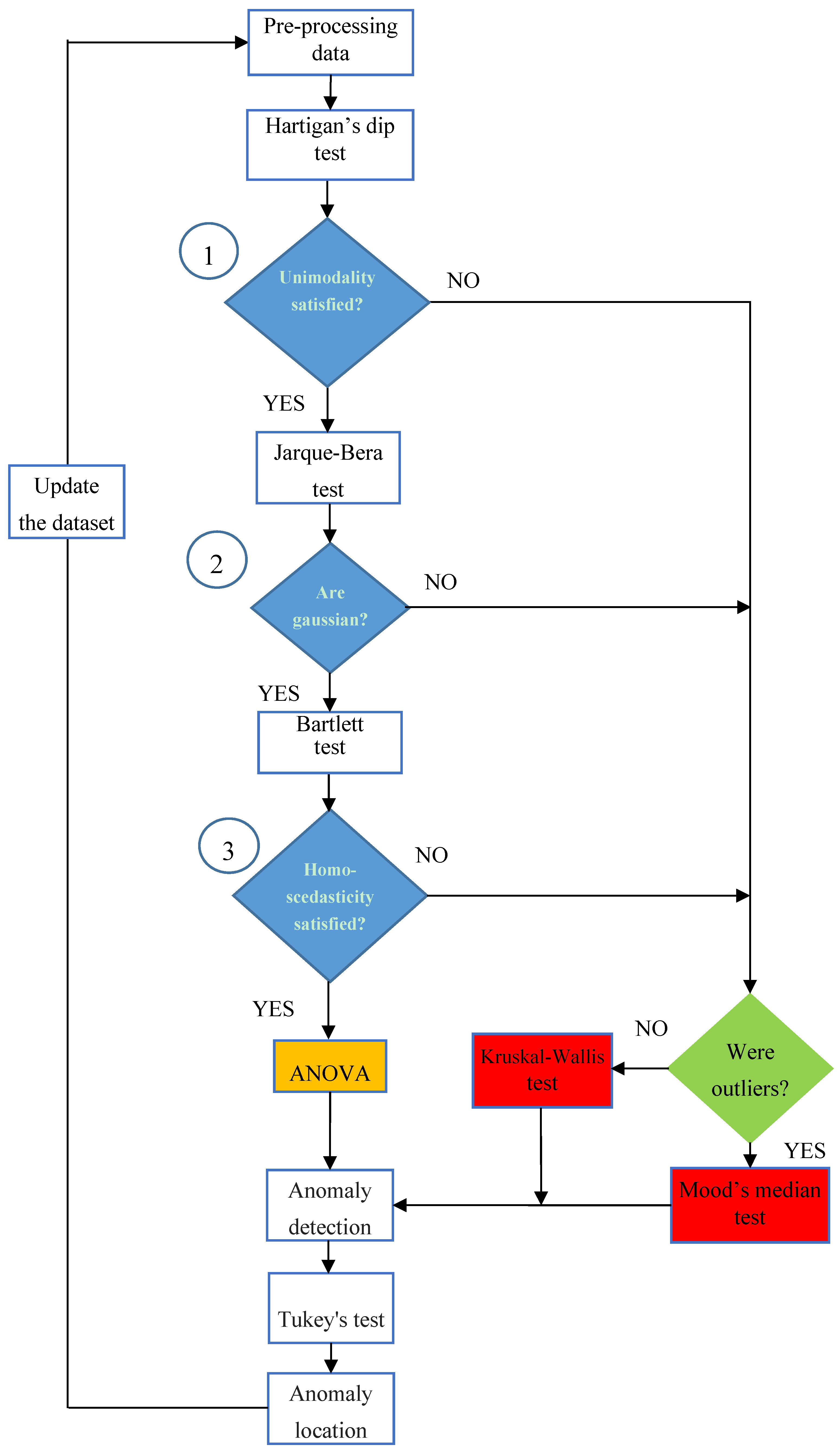
Figure 2 proposes the methodology to detect and locate any anomaly, before it becomes a fault.
It is based on the mutual comparison among the energy distributions of the arrays; therefore the environmental data are not necessary. Obviously, this approach is valid only if the arrays are identical (same PV modules, same number of modules for each array, same slope, same tilt, same inverter, and so on); in fact, under this assumption, the energy produced by any array must be almost equal to the energy produced by any other array of the same PV plant, in each period as well as in the whole year (the changing environmental conditions affect the arrays in the same way, if they are installed next to each other without any specific obstacle).
Thus, the comparative and cumulative monitoring of the energy performance of identical arrays allows one to determine, within the uncertainty defined by the value of the significance level α, if the arrays are producing the same energy or not. The first step of Figure 2 is the pre-processing of the energy dataset collected as previously explained, in order to check if outliers are present; the information about the presence or not of the outliers will be also useful later (green block). By default, an outlier is a value that is more than three scaled Median Absolute Deviations (MAD) away from the median. For a random dataset X = [ X 1 , X 2 , , X D ] , the scaled MAD is defined as:
M A D = F × m e d i a n ( | X j m e d i a n ( X ) | ) for   j = 1 , , D
where F is the scaling factor and is approximately 1.4826 for a normal distribution.
After the data pre-processing, it is necessary to verify if the arrays have produced the same amount of energy. This goal can be pursued by using parametric tests or non-parametric tests. As the parametric tests are based on a known distribution of the dataset, they are more reliable than the non-parametric ones, which are, instead, distribution-free. For this reason, it is advisable to use always the parametric tests, provided that all the needed assumptions are satisfied.
In particular, the parametric test known as ANOVA calculates the ratio between the variance among the arrays’ distributions (divided by the freedom degree) and the variance within each array distribution (divided by the freedom degree). In other words, ANOVA evaluates whether the differences of the mean values of the different groups are statistically significant or not. For this aim, ANOVA calculates the following Fisher’s statistic, F, [35]:
F = D A 1 · k = 1 A ( x ¯ k X ¯ ) 2 1 A ( D 1 ) · k = 1 A j = 1 D ( x k j x ¯ k ) 2
where x ¯ k is the mean value of the k-th distribution, X ¯ the global mean, x k j the j-th occurrence of the k-th distribution. The cumulative distribution function F allows to determine a p-value, which has to be compared with the significance level α, as later explained.
ANOVA is based on the null hypothesis H0 (Equation (4)) that the means of the distributions, μ k , are equal:
H 0 :   μ 1 = μ 2 = μ 3 = = μ A
versus the alternative hypothesis that the mean value of at least one distribution is different from the others. The output of the ANOVA test, as any other hypothesis test, is the p-value, which has to be compared with the pre-fixed significance value α. Usually, α = 0.05, so, if p-value < α then the null hypothesis is rejected, considering acceptable to have a 5% probability of incorrectly rejecting the null hypothesis (this is known as type I error).
Smaller values of α are not advisable to study the data of a medium-large PV plant, because the complexity of the whole system requires a larger uncertainty to be accepted. Nevertheless, ANOVA can be used only under the following assumptions:
(a)
all the observations are mutually independent;
(b)
all the distributions are normally distributed;
(c)
all the distributions have equal variance.
Finally, ANOVA can be applied also for limited violations of the assumptions (b) and (c), whereas the assumption (a) is always verified, if the measures come from independent local measurement units. So, before applying ANOVA test, several verifications are needed and they are represented by the three blue blocks of 
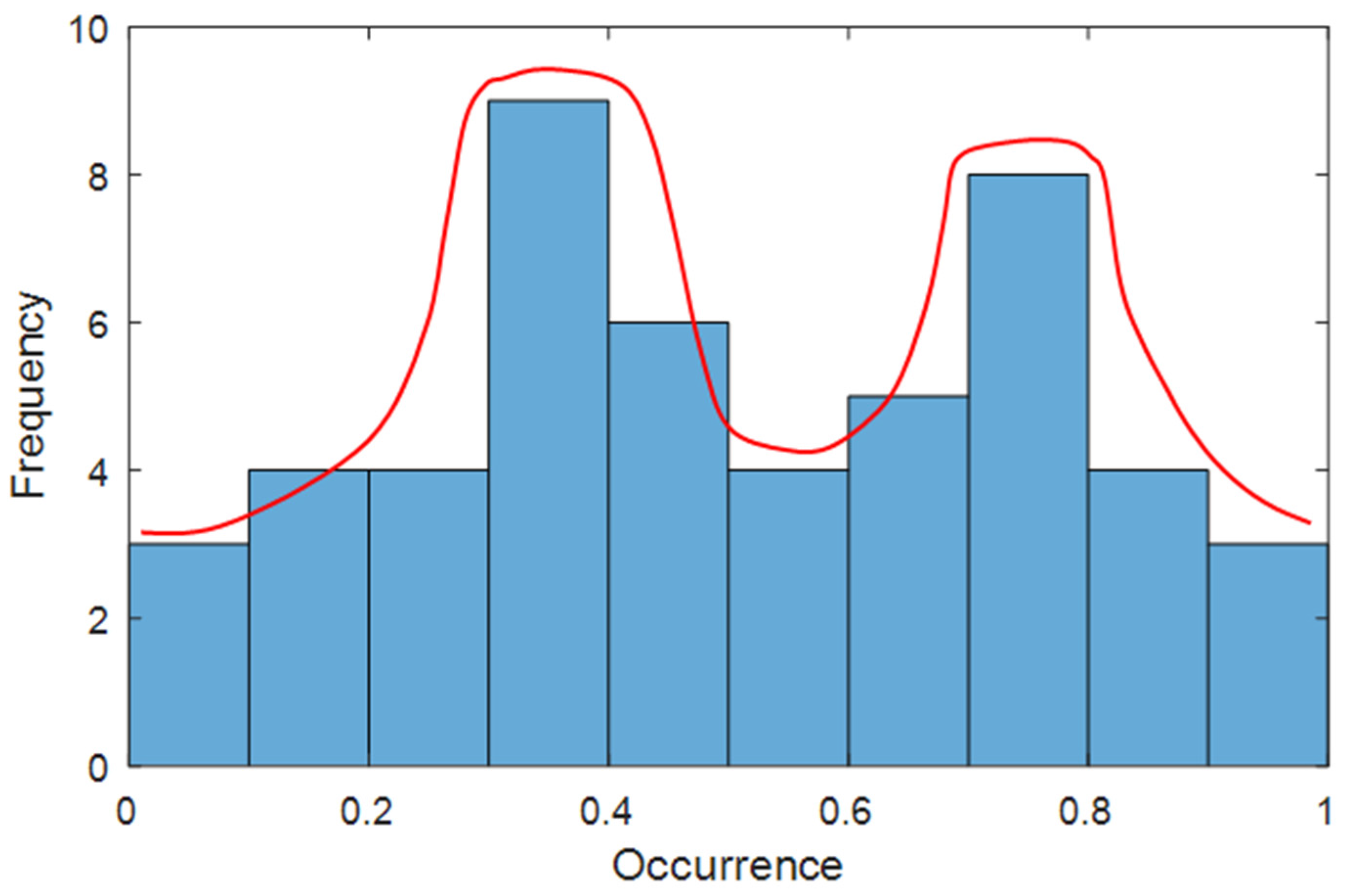
Figure 2. The first check (blue block 1) regards the unimodality of the dataset of each array, because a multimodality distribution, e.g., the bimodal distribution in Figure 3, is surely not Gaussian and violates the condition (b). Moreover, the daily-based energy distribution of an array of a well-working PV system is unimodal, because the daily solar radiation has the typical Gaussian waveform, which is unimodal; therefore, the multimodality of a daily-based energy distribution is a clear alert of a high-intensity anomaly. The Hartigan’s Dip Test (HDT) is able to check the unimodality [36] and is based on the null hypothesis that the distribution is unimodal versus the alternative one that it is at least bi-modal. The HDT is a non-parametric test, so it is distribution-free. HDT return a p-valueHDT. By fixing the significance value α = 0.05, if p-valueHDT < α is satisfied, the null hypothesis of the unimodality is rejected, the distribution is surely not Gaussian, ANOVA cannot be applied and a nonparametric test has to be used.
In the general case of A arrays, with A > 2, the nonparametric test has to be chosen between Kruskal-Wallis test (K-W) [37,38] and Mood’s Median test (MM), under the constraint of the green block; both K-W and MM do not require that the distributions are Gaussian, but only that the distributions are continuous.
In the presence of outliers (detected, if present, in the first block), MM performs better than K-W, otherwise K-W is a good choice. Both K-W and MM are based on the null hypothesis that the median values of all the distributions are equal versus the alternative one that at least one distribution has a median value different from the others. As K-W as MM returns a p-valueK-W(MM) that has to be compared with the significance value α = 0.05. If p-valueK-W(MM) < α is satisfied, the null hypothesis is rejected and the arrays have not produced the same energy; otherwise, they have. Instead, if the unimodality is satisfied, other checks are needed, before deciding whether ANOVA can be applied. In fact, it is needed to verify the previous assumptions (b) and (c). Only if both of them are satisfied (blue blocks 2 and 3, respectively), ANOVA can be applied.
To check the condition (b), an effective statistical tool is the Jarque-Bera’s Test (JBT). The JBT is distribution-free and based on independent random variable. It is a hypothesis test, whose null hypothesis is that the distribution is gaussian. Then, it calculates a statistical parameter, called JB, and returns a p-valueJBT. By fixing the significance value α = 0.05, if p-valueJBT < α is satisfied, the null hypothesis is rejected and the distribution is not gaussian, otherwise it is. It results:
JB = D 6 · [ σ k 2 + k u 2 4 ]
Being D the sample size, σ k the skewness and k u the Pearson’s kurtosis less 3 (also known as excess kurtosis). The skewness is defined as:
σ k = 1 D j = 1 D ( x j x ¯ ) 3 ( σ ^ 2 ) 3 2
Being D the sample size, x ¯ = 1 D j = 1 D x j the mean value, and σ ^ 2 = 1 D j = 1 D ( x j x ¯ ) 2 the variance. The skewness is the third standardized moment and measures the asymmetry of the data around the mean value. Only for σ k = 0 the distribution is symmetric; this is a necessary but not sufficient condition for a gaussian distribution. In fact, while the Gaussian distribution is surely symmetric, nevertheless there exist also symmetric but not gaussian distributions.
The excess kurtosis, instead, is defined as:
k u = 1 D j = 1 D ( x j x ¯ ) 4 ( σ ^ 2 ) 2 3
with the previous meaning of the parameters. The kurtosis is the fourth standardized moment and measures the tailedness of the distribution. Only for k u = 0 , the distribution is mesokurtic, which is the necessary but not sufficient condition for a Gaussian distribution. If the check of the blue block 2 is not passed, a non-parametric test (K-W or MM) has to be used, in accordance with the green block. Instead, if this verification is passed, it needs to test the assumption (c) of ANOVA, i.e., the homoscedasticity (blue block 3). This assumption can be verified by means of the Bartlett’s Test (BT), which is again a hypothesis test that returns a p-valueBT. The BT is effective for Gaussian distributions; in fact, in the flow-chart of Figure 2 it is used only if the distributions are Gaussian. Also in this case, it is possible to fix the common significance value α = 0.05 and to compare it with the p-valueBT. If the inequality p-valueJBT < α is satisfied, the null hypothesis is rejected and the variances of the distributions of the arrays are different, then the condition (c) is violated, and ANOVA cannot be applied. In this case, it is necessary to use K-W or MM, in accordance with the green block. Otherwise, ANOVA can be applied and it return another p-valueAN that must be compared with the significance level α = 0.05. If the inequality p-valueAN < α = 0.05 is satisfied, then the null hypothesis ( H 0 :   μ 1 = μ 2 = μ 3 = = μ A ) is rejected and the conclusion is that the identical arrays have not produced the same amount of energy; so, a low-intensity anomaly is present and it is located in the array that has the mean value different from the other ones. To detect it, a multi-comparison analysis—one-to-one—between the distributions is done by means of the Tukey’s Test (TT), which is a modified version of the well-known t-test and returns a p-valueTT, which states whether the means between two distributions are equal or not. For a small sample size (about 20 samples) the TT is reliable only for normal distribution, instead, for a lager sample size it is valid also for not normal distributions, because of the central limit theorem. Otherwise, no criticality is present and the dataset can be updated with new data to continue the monitoring of the PV plant. As the energy dataset increases, the monitoring becomes more accurate.

3. Description of the PV Plant under Investigation

The system under examination is a real operating 49.5 kWp grid-connected PV plant, installed in the south of Italy on the roof of the industrial building of a company. The PV plant has been designed and installed under the scheme of the feed-in tariff, financed by the Government. The 330 modules of the PV plant are equally divided in five arrays, each of them constituted by 66 PV modules. The nominal peak power of a single module is 150 W, and then the nominal peak power of a single array is 9.9 kWp. Each array is connected to the grid via a 10 kW inverter. The system faces the south and the slop is about 30°. By inserting these values in the previously mentioned PVGIS [31] of the EC-JRC, it results that the estimated yearly energy production is about 64,724 kWh, corresponding to about 1307 kWh/kWp per year. Moreover, the website provides also the estimated monthly energy production, which will be used in the next Section 4.1, Section 4.2, and Section 4.3. The PV plant is equipped with a datalogger that stores the data from the five arrays. The datalogger has a sample time of 2 s. After 10 min, the measured samples are equal to 30 (samples/min) × 10 (min) = 300 samples; an internal software calculates the average value of these 300 measured samples, whereas the energy produced in this time-slot of 10 min is calculated as P a v e r a g e · 10 60 [ k W h ] . This value is stored into the datalogger. So, the sampling time of the energy is 10 min, therefore there are 6 samples/hour, hence 144 samples/day, that are summed in the proposed procedure. Thus, the unique value of a day is not an average value, but a cumulative data that takes into account the variability of the environmental conditions happened during the whole day.
The measured variables are the power in AC, the energy in AC, and the voltage Vdc of each inverter; moreover, the number of the operating hours is stored. The default monitoring system of the PV plant uses the power in AC and the voltage Vdc, the daily and total energy produced by each inverter, and the number of the operating hours. It is worth noting that the monitoring system is an internal software of the datalogger. As the operation of the monitoring system occupies the internal memory, for default the internal monitoring system does not utilize all the data available into the datalogger, in order not to occupy the internal memory quickly. This approach allows to monitor the PV plant for a longer time, but only the high-intensity anomalies can be detected. Instead, to detect even the low-intensity anomalies, it is necessary to use the methodology described in Figure 2 and all the data stored into the datalogger. Moreover, even if the measurement system of this PV plant does not measure all the variables mentioned in the Section 2 (the produced energy, other than the voltage and current in both the DC and AC side), nevertheless it acquires the produced energy that is the unique variable necessary for the proposed methodology; so it can be applied. The observation period refers to a full year during which the plant has shown some malfunctions, whereas in the previous years the PV plant has not shown any malfunctions, therefore the results of the previous years are not reported in the paper.

4. Cumulative Statistical Analysis

The energy performance of the PV plant described in Section 3 has been studied by means of the statistical methodology proposed in Section 2. Statistical data analysis has been carried out in Matlab R2017 environment by using the standard routines of the Statistics toolbox and by implementing the flow chart of Figure 2. In particular, a Matlab routine that implements just the procedure of Figure 2 has been written and run for each analysis discussed later. As some tests (ANOVA, K-W, JBT) are implemented in the Statistics Toolbox of Matlab, these native-routines are recalled from the main routine, when necessary. As already explained, each array is equipped by a devoted measurement system, then the five distributions are mutually independent.
Four analyses are discussed, based on the dataset of the energy produced by each array:
  • one-month analysis (January);
  • three-months analysis (January–March);
  • six-months analysis (January–June);
  • one-year analysis (January–December).
The increase of the time window, updating the dataset as described in Figure 2, allows understanding how some characteristic benchmarks of the PV plants vary during the year, as new data are acquired. The following results will be reported for each analysis: the p-valueHDT of each distribution to test the unimodality; the p-valueJBT of each distribution to test whether each one of them is gaussian; the p-valueBT to test the homoscedasticity among the distributions; the p-valueAN to test whether all the distributions have the same mean value; the p-valueK-W(MM) of the non-parametric test (when ANOVA cannot be applied) to check whether all the distributions have the same median value; the box plot of the ANOVA test or of the non-parametric test; the mean value of each distribution and its spread with respect to the global mean of the PV plant.

4.1. One-Month Analysis (January)

Table 1 reports the main numerical values of the parameters calculated by applying the procedure in Figure 2.
This dataset is constituted by 31 cumulative samples/array, each sample being the sum of 144 samples/day. The energy dataset of the first month does not contain outliers. The p-valueHDT > α = 0.05 for each distribution, so all the distributions are unimodal. To apply ANOVA, conditions (b) and (c) have to be verified.
Table 1 reports the JB values and the related p-valueJBT; as p-valueJBT > α = 0.05, all the distributions are Gaussian, so condition (b) of ANOVA is satisfied. Condition (c) about the homoscedasticity has to be verified by means of BT (see Figure 2). The p-valueBT = 0.999 in Table 1 (again higher than α = 0.05) says that the homoscedasticity is verified, then all the variances are equal. Therefore, the main conditions of the flow chart in Figure 2 (blocks 1,2,3) are satisfied and ANOVA can be applied. The p-valueAN = 0.999 in Table 1 says that the distributions have the same mean values, so all the arrays have produced the same energy in this month. Figure 4 is the box plot of ANOVA. For each box, the central red mark indicates the median, and the bottom and top edges of the box indicate the 25th and 75th percentiles, respectively. The whiskers extend to the most extreme data points. Figure 4 highlights that the five distributions have produced almost the same energy, both with respect to the median value (in red color) and to the first and third inter-quartiles; moreover, outliers are absent. Therefore, no anomaly is present in the PV plant. Particularly, from PVGIS [31], it results that the estimated average energy of the PV plant in January should be about 3173 kWh, corresponding to a daily average energy for each array of about 3173/(31 × 5) = 20.5 kWh, that is almost equal to the global mean value 19.74 kWh of Table 1. Figure 5 diagrams the mean value and confidence interval at 95% of each distribution; the values are very similar each other, as it results also from Table 2 that reports the one-to-one comparisons of the mean values. In particular, the high p-values confirm that the differences are not significant.

4.2. Three-Months Analysis (January–March)

Table 3 reports the main numerical values of the parameters calculated by following the algorithm of Figure 2 for the energy dataset of three months, including the first month already considered in the previous analysis. This dataset is constituted by 90 cumulative samples/array, each sample being the sum of 144 samples/day. The p-valueHDT > α = 0.05 for each distribution, so all the distributions are still unimodal. The p-valueJBT > α = 0.05, so all the distributions are gaussian and the condition (b) of ANOVA is satisfied. The homoscedasticity is also satisfied (p-valueBT > α = 0.05). Therefore, the main conditions of the flow chart in Figure 2 (blocks 1,2,3) are satisfied and ANOVA can be newly applied. The p-valueAN = 0.998 affirms that the distributions have the same mean values, so all the arrays have produced the same energy also in these three months. Figure 6 is the box plot of ANOVA and it highlights that the five distributions have produced almost the same energy, both with respect to the median value (in red color) and to the first and third inter-quartiles; moreover, outliers are not present. Therefore, no anomaly is present in the PV plant in these three months. Particularly, from PVGIS [31], it results that the estimated average energy of the PV plant in the period January–June should be about 11,695 kWh, corresponding to a daily average energy for each array of about 11,695/(90 × 5) = 25.99 kWh, that is almost equal to the global mean value 25.95 kWh of Table 2.
Figure 7 plots the mean value and confidence interval at 95% of each distribution; the values are very similar each other, as it results also from Table 4 that reports the one-to-one comparisons of the mean values. In particular, the high p-values confirm that the differences are not significant.

4.3. Six-Months Analysis (January–June)

Table 5 displays the main numerical values of the parameters obtained by the application of the procedure in Figure 2, after updating the previous energy dataset (used for the January–March analysis), by adding the data of the successive three months. This dataset is constituted by 181 cumulative samples/array, each sample being the sum of 144 samples/day. The pre-processing of the new dataset has excluded the presence of outliers. The p-valueHDT > α = 0.05 for each distribution, so all the distributions are still unimodal. As p-valueJBT < α = 0.05 for each distribution, then the null hypothesis is rejected and the constraint of the block 2 (corresponding to the condition (b) of ANOVA) is not satisfied: the distributions are not Gaussian. Therefore, it has no sense to verify the homoscedasticity, because it is mandatory to use a nonparametric test. As no outlier is present, it is advisable to use K-W, as suggested by the green block. The p-valueK-W = 0.861 affirms that the distributions have the same median values, so all the arrays have produced the same energy also in these six months, even if the distributions are no longer Gaussian. Figure 8 is the box plot of K-W and it highlights that the five distributions have produced almost the same energy, both with respect to the median value (in red color) and to the first and third inter-quartiles; moreover, it is confirmed that outliers are not present. Therefore, no anomaly is present in the PV plant in these six months. Particularly, from PVGIS [31], it results that the estimated average energy of the PV plant in the period January–June should be about 32,285 kWh, corresponding to a daily average energy for each array of about 32,285/(181 × 5) = 35.67 kWh, that is almost equal to the global mean value 36.23 kWh of Table 3. Figure 9 illustrates the mean value and confidence interval at 95% of each distribution; the values are very similar each other, as it results also from Table 6 that reports the one-to-one comparisons of the mean values. In particular, the high p-values confirm that the differences are not significant.

4.4. One-Year Analysis (January–December)

Table 7 displays the main numerical values of the parameters obtained by the application of the procedure in Figure 2, after updating the previous energy dataset (used for the January–June analysis), by adding the data of the successive six months. This dataset is constituted by 365 cumulative samples/array, each sample being the sum of 144 samples/day. The pre-processing of the new dataset has excluded the presence of outliers. The p-valueHDT > α = 0.05 for each distribution, except for the distribution n. 4, for which p-valueHDT(4) = 0.006 < α = 0.05; therefore, the condition of the block 1 about the unimodality is not satisfied for all the distributions and ANOVA cannot be applied. Consequently, it is mandatory to use a nonparametric test. As no outlier is present, it is advisable to apply K-W, as suggested by the green block. As p-valueK-W = 0.009 < α = 0.05, the null hypothesis is rejected, so the distributions have different median values. This implies that the arrays have not produced the same energy in the complete year, even if they had produced the same energy for the first six months. Figure 10 is the box plot of K-W and it highlights that the median value of the distribution n. 4 is significantly different from the others. It is also confirmed that outliers are not present. Particularly, from PVGIS [31], it results that the estimated average energy of the PV plant in the period January–December should be about 64,724 kWh, corresponding to a daily average energy for each array of about 64,724/(365 × 5) = 35.46 kWh, that is almost equal to the global mean value 35.13 kWh of Table 4. Therefore, high-intensity anomaly is not present, but a low-intensity anomaly is detected in the array n. 4, as confirmed also by the spreads of the mean values reported in Table 4. It can be observed that the array n. 4 produced 6.54% less than the average energy of the PV plant. Figure 11 shows the mean value and confidence interval at 95% of each distribution. It can be observed that the array n. 4 is very different from the other ones, as it results also from Table 8 that reports the one-to-one comparisons of the mean values. In particular, the p-value 0.043 < α = 0.05 rejects the hypothesis that the distribution 4 and 5 have the same mean value.

5. Conclusions

The paper proposes a statistical algorithm to monitor the energy performance of PV plants and detect anomalies. The procedure is cumulative and the algorithm can be iterated, as new data are acquired by the measurement system, in order to follow the most important benchmarks. The case study, referred to a real operating PV system, has shown the results of four cumulative analyses, starting from the dataset of only one month and finishing with a yearly-based dataset. As real operating PV systems are affected by atmospheric phenomena, their energy distributions are never perfectly Gaussian, so parametric tests should never be applied. Instead, as ANOVA can be applied for modest violations of its assumptions, the issue consists in evaluating the violation, in order to decide whether it is negligible or not. The proposed methodology, based on hypothesis tests, allows this evaluation. The first two analyses (based on the data of one and three months, respectively) have been carried out by means of the parametric test ANOVA, whereas the third and the fourth analyses have been based on the nonparametric test K-W, because the mandatory ANOVA’s assumptions were not satisfied. Moreover, while the first three analyses have not evidenced any anomaly in the PV plant—in fact the energy distributions of the arrays were almost equal—instead the last analysis has shown a not negligible anomaly in the array n. 4. The proposed methodology does not allow identifying the origin of the anomaly, but only to detect and locate it. Finally, the proposed procedure is particularly effective in absence of environmental parameters, i.e., for monitoring PV plants not equipped with a weather station. In this case, the procedure allows extracting the main operating features of the PV plants without adding new hardware; thus, this approach is also cheap. Nevertheless, when a commercial PV plant has to be evaluated, it is mandatory to take into account the environmental parameters; so, if the PV plant is not equipped by a weather station, it is necessary to add this component and to use the monitoring methodologies based on the environmental data, even though this results more expensive.

Conflicts of Interest

The author declares no conflict of interest.

References

  1. Xiao, W.; Ozog, N.; Dundorf, W.G. Topology study of photovoltaic interface for maximum power point tracking. IEEE Trans. Ind. Electron. 2007, 54, 1696–1704. [Google Scholar] [CrossRef]
  2. Mutoh, N.; Inoue, T. A control method to charge series-connected ultraelectric double-layer capacitors suitable for photovoltaic generation systems combining MPPT control method. IEEE Trans. Ind. Electron. 2007, 54, 374–383. [Google Scholar] [CrossRef]
  3. Grimaccia, F.; Leva, S.; Mussetta, M.; Ogliari, E. ANN Sizing Procedure for the Day-Ahead Output Power Forecast of a PV Plant. Appl. Sci. 2017, 7, 622. [Google Scholar] [CrossRef]
  4. Dellino, G.; Laudadio, T.; Mari, R.; Mastronardi, N.; Meloni, C.; Vergura, S. Energy Production Forecasting in a PV Plant Using Transfer Function Models. In Proceedings of the 2015 IEEE 15th International Conference on Environment and Electrical Engineering (EEEIC), Roma, Italy, 10–13 June 2015. [Google Scholar]
  5. Vergura, S.; Pavan, A.M. On the photovoltaic explicit empirical model: Operations along the current-voltage curve. In Proceedings of the 2015 International Conference on Clean Electrical Power (ICCEP), Taormina, Italy, 16–18 June 2015. [Google Scholar]
  6. Guerriero, P.; di Napoli, F.; Vallone, G.; D’Alessandro, V.; Daliento, S. Monitoring and diagnostics of PV plants by a wireless self-powered sensor for individual panels. IEEE J. Photovolt. 2015, 6, 286–294. [Google Scholar] [CrossRef]
  7. Takashima, T.; Yamaguchi, J.; Otani, K.; Kato, K.; Ishida, M. Experimental Studies of Failure Detection Methods in PV module strings. In Proceedings of the 2006 IEEE 4th World Conference on Photovoltaic Energy Conversion, Waikoloa, HI, USA, 7–12 May 2006; Volume 2, pp. 2227–2230. [Google Scholar]
  8. Breitenstein, O.; Rakotoniaina, J.P.; Al Rifai, M.H. Quantitative evaluation of shunts in solar cells by lock-in thermography. Prog. Photovolt. Res. Appl. 2003, 11, 515–526. [Google Scholar] [CrossRef]
  9. Grimaccia, F.; Leva, S.; Dolara, A.; Aghaei, M. Survey on PV Modules’ Common Faults after an O&M Flight Extensive Campaign over Different Plants in Italy. IEEE J. Photovolt. 2017, 7, 810–816. [Google Scholar]
  10. Johnston, S.; Guthrey, H.; Yan, F.; Zaunbrecher, K.; Al-Jassim, M.; Rakotoniaina, P.; Kaes, M. Correlating multicrystalline silicon defect types using photoluminescence, defect-band emission, and lock-in thermography imaging techniques. IEEE J. Photovolt. 2014, 4, 348–354. [Google Scholar] [CrossRef]
  11. Peloso, M.P.; Meng, L.; Bhatia, C.S. Combined thermography and luminescence imaging to characterize the spatial performance of multicrystalline Si wafer solar cells. IEEE J. Photovolt. 2015, 5, 102–111. [Google Scholar] [CrossRef]
  12. Vergura, S.; Marino, F. Quantitative and Computer Aided Thermography-based Diagnostics for PV Devices: Part I—Framework. IEEE J. Photovolt. 2017, 7, 822–827. [Google Scholar] [CrossRef]
  13. Vergura, S.; Colaprico, M.; de Ruvo, M.F.; Marino, F. A Quantitative and Computer Aided Thermography-based Diagnostics for PV Devices: Part II—Platform and Results. IEEE J. Photovolt. 2017, 7, 237–243. [Google Scholar] [CrossRef]
  14. Mekki, H.; Mellit, A.; Salhi, H. Artificial neural network-based modelling and fault detection of partial shaded photovoltaic modules. Simul. Model. Pract. Theory 2016, 67, 1–13. [Google Scholar] [CrossRef]
  15. Harrou, F.; Sun, Y.; Kara, K.; Chouder, A.; Silvestre, S.; Garoudja, E. Statistical fault detection in photovoltaic systems. Sol. Energy 2017, 150, 485–499. [Google Scholar]
  16. Vergura, S.; Carpentieri, M. Statistics to detect low-intensity anomalies in PV systems. Energies 2018, 11, 30. [Google Scholar]
  17. Ventura, C.; Tina, G.M. Development of models for on line diagnostic and energy assessment analysis of PV power plants: The study case of 1 MW Sicilian PV plant. Energy Procedia 2015, 83, 248–257. [Google Scholar] [CrossRef]
  18. Silvestre, S.; Kichou, S.; Chouder, A.; Nofuentes, G.; Karatepe, E. Analysis of current and voltage indicators in grid connected PV (photovoltaic) systems working in faulty and partial shading conditions. Energy 2015, 86, 42–50. [Google Scholar] [CrossRef]
  19. Vergura, S. A Complete and Simplified Datasheet-based Model of PV Cells in Variable Environmental Conditions for Circuit Simulation. Energies 2016, 9, 326. [Google Scholar] [CrossRef]
  20. Vergura, S. Scalable Model of PV Cell in Variable Environment Condition based on the Manufacturer Datasheet for Circuit Simulation. In Proceedings of the 2015 IEEE 15th International Conference on Environment and Electrical Engineering (EEEIC), Roma, Italy, 10–13 June 2015. [Google Scholar]
  21. Chao, K.H.; Ho, S.H.; Wang, M.H. Modeling and fault diagnosis of a photovoltaic system. Electr. Power Syst. Res. 2008, 78, 97–105. [Google Scholar] [CrossRef]
  22. Hamdaoui, M.; Rabhi, A.; Hajjaji, A.; Rahmoum, M.; Azizi, M. Monitoring and control of the performances for photovoltaic systems. In Proceedings of the International Renewable Energy Congress, Sousse, Tunisia, 5–7 November 2009. [Google Scholar]
  23. Kim, I.-S. On-line fault detection algorithm of a photovoltaic system using wavelet transform. Sol. Energy 2016, 226, 137–145. [Google Scholar] [CrossRef]
  24. Rabhia, A.; El Hajjajia, A.; Tinab, M.H.; Alia, G.M. Real time fault detection in photovoltaic systems. Energy Procedia 2017, 11, 914–923. [Google Scholar]
  25. Plato, R.; Martel, J.; Woodruff, N.; Chau, T.Y. Online fault detection in PV systems. IEEE Trans. Sustain. Energy 2015, 6, 1200–1207. [Google Scholar] [CrossRef]
  26. Ando, B.; Bagalio, A.; Pistorio, A. Sentinella: Smart monitoring of photovoltaic systems at panel level. IEEE Trans. Instrum. Meas. 2015, 64, 2188–2199. [Google Scholar] [CrossRef]
  27. Harrou, F.; Sun, Y.; Taghezouit, B.; Saidi, A.; Hamlati, M.E. Reliable fault detection and diagnosis of photovoltaic systems based on statistical monitoring approaches. Renew. Energy 2018, 116, 22–37. [Google Scholar] [CrossRef]
  28. International Electrotechnical Commission (IEC). Photovoltaic System Performance Monitoring—Guidelines for Measurement, Data Exchange and Analysis, International Standard 61724, 1st ed.; International Electrotechnical Commission (IEC): Geneva, Switzerland, 1998. [Google Scholar]
  29. Leloux, J.; Narvarte, L.; Trebosc, D. Review of the performance of residential PV systems in Belgium. Renew. Sustain. Energy Rev. 2012, 16, 178–184. [Google Scholar] [CrossRef] [Green Version]
  30. Leloux, J.; Narvarte, L.; Trebosc, D. Review of the performance of residential PV systems in France. Renew. Sustain. Energy Rev. 2012, 16, 1369–1376. [Google Scholar] [CrossRef] [Green Version]
  31. Available online: http://re.jrc.ec.europa.eu/pvg_tools/en/tools.html (accessed on 20 January 2018).
  32. Rohatgi, V.K.; Szekely, G.J. Sharp inequalities between skewness and kurtosis. Stat. Probab. Lett. 1989, 8, 297–299. [Google Scholar] [CrossRef]
  33. Klaassen, C.A.J.; Mokveld, P.J.; van Es, B. Squared skewness minus kurtosis bounded by 186/125 for unimodal distributions. Stat. Probab. Lett. 2000, 50, 131–135. [Google Scholar] [CrossRef]
  34. Hogg, R.V.; Ledolter, J. Engineering Statistics; MacMillan: Basingstoke, UK, 1987. [Google Scholar]
  35. Roussas, G. An Introduction to Probability and Statistical Inference; Academic Press: Cambridge, MA, USA, 2015. [Google Scholar]
  36. Hartigan, J.A.; Hartigan, P.M. The dip test of unimodality. Ann. Stat. 1985, 13, 70–84. [Google Scholar] [CrossRef]
  37. Gibbons, J.D. Nonparametric Statistical Inference, 2nd ed.; M. Dekker: New York, NY, USA, 1985. [Google Scholar]
  38. Hollander, M.; Wolfe, D.A. Nonparametric Statistical Methods; Wiley: Hoboken, NJ, USA, 1973. [Google Scholar]
Figure 1. PVGIS of the European Commission Joint Research Centre (EC-JRC).
Energies 11 00485 g001
Figure 2. Statistical methodology.
Energies 11 00485 g002
Figure 3. Example of histogram of a bimodal distribution.
Energies 11 00485 g003
Figure 4. Box plot of ANOVA test of the five distributions for the one-month analysis (January).
Energies 11 00485 g004
Figure 5. Mean value of the energy produced by each array for the one-month analysis (January).
Energies 11 00485 g005
Figure 6. Box plot of K-W test of the five distributions for the three-months analysis (January–March).
Energies 11 00485 g006
Figure 7. Mean value of the energy produced by each array for the three-months analysis (January–March).
Energies 11 00485 g007
Figure 8. Box plot of K-W test of the five distributions for the six-months analysis (January–June).
Energies 11 00485 g008
Figure 9. Mean value of the energy produced by each array for the three-months analysis (January–June).
Energies 11 00485 g009
Figure 10. Box plot of K-W test of the five distributions for the one-year analysis.
Energies 11 00485 g010
Figure 11. Mean value of the energy produced by each array for the one-year analysis.
Energies 11 00485 g011
Table 1. p-Value of HDT, JBT, BT, ANOVA for the energy distribution of the arrays, and mean in kWh and spread with respect to the global mean for one-month analysis (January).
Array Number12345
p-valueHDT0.6280.3640.6740.6580.670
JBTJB0.6990.6760.6740.7180.638
p-valueJBT0.5000.5000.5000.5000.500
p-valueBT0.999
p-valueAN0.999
Mean (kWh)19.5919.9019.9119.4619.84
Global mean19.74
Spread %−0.760.800.85−1.400.51
Table 2. One-to-one comparison of the means for the one-month analysis (January).
Comparison between SamplesLowerBoundDifferenceEstimateUpperBoundp-ValueTT
12−8.77−0.318.160.999
13−8.78−0.328.150.999
14−8.340.128.590.999
15−8.71−0.258.210.999
23−8.47−0.018.451
24−8.030.438.900.999
25−8.410.068.521
34−8.020.448.910.999
35−8.400.068.531
45−8.84−0.388.090.999
Table 3. p-Value of HDT, JBT, BT, ANOVA for the energy distribution of the arrays, and mean in kWh and spread with respect to the global mean for three-month analysis (January–March).
Array Number12345
p-valueHDT0.7760.8920.8180.8560.830
JBTJB5.1275.1985.1145.1775.090
p-valueJBT0.0540.0530.0540.0530.055
p-valueBT0.999
p-valueAN0.998
Mean (kWh)25.8425.8226.2325.6226.39
Global mean25.95
Spread %−0.54−0.620.98−1.361.58
Table 4. One-to-one comparison of the means for the three-months analysis (January–March).
Comparison between SamplesLowerBoundDifferenceEstimateUpperBoundp-ValueTT
12−6.680.026.731
13−7.10−0.396.310.999
14−6.490.216.920.999
15−7.25−0.556.150.999
23−7.12−0.416.290.999
24−6.510.196.900.999
25−7.27−0.576.130.999
34−6.090.607.310.999
35−6.86−0.156.550.999
45−7.47−0.765.940.997
Table 5. p-Value of HDT, JBT, BT, (KW) for the energy distribution of the arrays, and mean in kWh and spread with respect to the global mean for six-months analysis (January–June).
Array Number12345
p-valueHDT0.7940.7220.7820.8080.842
JBTJB13.9514.0213.9213.9413.85
p-valueJBT0.0070.0070.0070.0070.007
p-valueBT------------
p-valueK-W0.861
Mean (kWh)36.0135.7836.6035.7437.04
Global mean36.23
Spread %−0.60−1.231.02−1.352.23
Table 6. One-to-one comparison of the means for the three-months analysis (January–June).
Comparison between SamplesLowerBoundDifferenceEstimateUpperBoundp-ValueTT
12−5.140.225.600.999
13−5.96−0.584.780.999
14−5.100.275.640.999
15−6.40−1.024.340.985
23−6.18−0.814.550.993
24−5.330.045.411
25−6.62−1.254.110.968
34−4.510.856.230.992
35−5.81−0.434.930.999
45−6.67−1.294.070.964
Table 7. p-Value of HDT and K-W for the energy distribution of the arrays, and mean in kWh and spread with respect to the global mean for one-year analysis.
Array Number
12345
p-valueHDT0.8200.8460.8980.0060.636
p-valueJBT-----
p-valueBT-----
p-valueK-W0.009
Mean (hWh)35.3735.2435.9232.8336.31
Global mean35.13
Spread %0.680.322.25−6.543.35
Table 8. One-to-one comparison of the means for the one-year analysis.
Comparison between SamplesLowerBoundDifferenceEstimateUpperBoundp-ValueTT
12−3.760.124.010.999
13−4.44−0.553.330.995
14−0.863.026.910.210
15−4.83−0.942.950.964
23−4.56−0.673.210.989
24−0.982.906.790.249
25−4.95−1.062.820.945
34−0.313.577.470.088
35−4.28−0.383.500.998
45−7.85−3.96−0.070.043

