Article

Analyzing and Forecasting Electrical Load Consumption in Healthcare Buildings

by
Rodolfo Gordillo-Orquera 
1,2,*,
Luis Miguel Lopez-Ramos
2,3,
Sergio Muñoz-Romero
2,4,
Paz  Iglesias-Casarrubios
5,
Diego Arcos-Avilés
1,
Antonio G. Marques
2 and
José Luis Rojo-Álvarez
2,3
1
Departamento de Eléctrica y Electrónica, Universidad de las Fuerzas Armadas—ESPE, 171-5-231B Sangolquí, Ecuador
2
Department of Signal Theory and Communications, Rey Juan Carlos University, 28943 Fuenlabrada, Spain
3
Wisenet Signal Processing & Wireless Networks laboratory, University of Agder, 4876 Grimstad, Norway
4
Center for Computational Simulation, Universidad Politécnica de Madrid; Boadilla, 28223 Madrid, Spain
5
Hospital Universitario de Fuenlabrada, 28492 Fuenlabrada, Spain
*
Author to whom correspondence should be addressed.
Energies 2018, 11(3), 493; https://doi.org/10.3390/en11030493
Submission received: 28 January 2018 / Revised: 13 February 2018 / Accepted: 22 February 2018 / Published: 26 February 2018

Abstract

:
Healthcare buildings exhibit a different electrical load predictability depending on their size and nature. Large hospitals behave similarly to small cities, whereas primary care centers are expected to have different consumption dynamics. In this work, we jointly analyze the electrical load predictability of a large hospital and that of its associated primary care center. An unsupervised load forecasting scheme using combined classic methods of principal component analysis (PCA) and autoregressive (AR) modeling, as well as a supervised scheme using orthonormal partial least squares (OPLS), are proposed. Both methods reduce the dimensionality of the data to create an efficient and low-complexity data representation and eliminate noise subspaces. Because the former method tended to underestimate the load and the latter tended to overestimate it in the large hospital, we also propose a convex combination of both to further reduce the forecasting error. The analysis of data from 7 years in the hospital and 3 years in the primary care center shows that the proposed low-complexity dynamic models are flexible enough to predict both types of consumption at practical accuracy levels.

1. Introduction

Electricity load forecasting is an active research topic with significant practical implications for almost any industry or organization. This is not surprising, as the accurate prediction of energy consumption and requirements has a positive impact on operational budgets [1]. In the case of the electrical industry, accurate electrical load forecasting is a useful tool to provide well-founded information and efficient energy management for planning in both the mid and long term and for the grid operation in the short term [2]. Depending on the prediction horizon (i.e., the lead time), forecasting problems are classified into three groups: short-term load forecasts (STLFs), which usually aim to predict the load consumption up to 1 week ahead; medium-term load forecasts (MTLFs), which cover from 1 week to 1 year; and finally, long-term load forecasts (LTLFs), which aim at load prediction for over a year ahead. Most of the studies in recent years have focused on the STLF category [3], whereas MTLFs and LTLFs have received less attention [4,5]. In addition, existing studies have mainly addressed load forecasting for utility companies, whereas fewer works have investigated forecasts for the customer side.
Because of their social relevance, size, and operational characteristics, healthcare buildings are a type of customer that deserves particular attention. However, little attention has been paid to the intuitive fact that their dynamics are considerably different from those of a utility or other middle/large-scale customers. In fact, utilities have shown more interest in predicting the aggregated load of a city, a region, or an entire country or state [6] than in forecasting the consumption of particular customers. Apart from their social relevance, analyzing the specific case of healthcare buildings is justified from multiple points of view. First, the energy needs of large hospitals are comparable to those of a small city. Second, we hypothesize that the load predictability in a hospital will be more accurate, as most systems are controlled in a centralized fashion rather than independently by hundreds or thousands of users. Moreover, because the healthcare activity is very specific, many intrinsic and extrinsic variables affecting the energy consumption are strongly seasonal, either directly (e.g., temperature increase in the summer) or indirectly (e.g., increased illness in the winter). Finally, demographic factors, such as the population age, epidemics, and public health information, are known to have a relevant impact on the health activity (e.g., types of attention, treatments, or duration of the patient staying), and health centers work under their population aggregation with different sizes depending on the health building service, size, and coverage.
To the best of our knowledge, no study has analyzed whether the dynamics of this composition become low complexity, which could be a result of average/aggregation effects, or high complexity, which could be a result of complicated interactions among the actors and elements in the system. The identification of the load complexity forecasting in a hospital can be also useful to propose adequate prediction systems, and if we also model the relationship among the relevant exogenous variables, the information concerning the hospital capacity (i.e., load elasticity), and the power consumption, then managers will be able to readily identify which tasks are more energy demanding. This will reduce the consumption for specific activities while allowing the managers to take advanced load management actions, such as investments in new equipment (e.g., heating, cooling, and ventilation) or even in real-time control systems. All these actions can be taken to achieve significant savings in the electric bill, and they depend on the load prediction accuracy in healthcare buildings [7].
Therefore, in this work, we aim to analyze the dynamics and predictability of the electrical load in healthcare buildings. For this purpose, we have compared the consumption in a large hospital to that of its main primary care center. This allowed us to have similar demographic, environmental, political, and epidemiological conditions. We scrutinized the dynamics of their middle- and short-term predictions, aiming to determine and assess their complexity. For this end, we used multivariate techniques that allowed us not only to predict but also to scrutinize the consumption. First, the intrinsic predictability was assessed using principal component analysis (PCA) and autoregressive (AR) modeling. Second, supervised modeling was addressed by using orthonormal partial least squares (OPLS). Finally, with the aim of improving the prediction capabilities, we also put forward a simple convex combination method that leveraged the PCA and OPLS predictions. After this, we analyzed consumption data from 7 years for the Hospital Universitario de Fuenlabrada (HUF) hospital and from 3 years for the Centro de Especialidades El Arroyo (CEA) primary care center, because of stored-data availability conditions; both are located in Fuenlabrada, Madrid (Spain).
The main contributions of this paper are detailed as follows. First, we performed the electrical load forecast for a 1 year horizon using multivariate analysis (MVA), by extracting a new set of representative features of the load consumption in the hospital and care center, which allowed us to analyze their time patterns. Second, the proposed forecasting algorithms were validated using real data from two different-sized healthcare buildings, which exhibited different patterns in terms of energy consumption but in both cases had low-complexity dynamics. Third, we proposed a simple convex combination to, whenever necessary, merge the supervised and unsupervised MVA approaches into a single method.
The rest of the paper is structured as follows. In Section 2, we detail the methodology used for MVA, including the unsupervised and supervised methods and the algorithms for generating the forecasted output. In Section 3, we describe the datasets considered in this work, corresponding to the two aforementioned healthcare buildings. In Section 4, we present the experiments together with their performance results, and a detailed description is included of the most descriptive components from the PCA and OPLS approaches, which allowed us to scrutinize the complexity of the dynamics. Finally, in Section 5, we present the discussion and main conclusions of this work.

2. Proposed Methodology

MVA methods are required when dealing with high-dimensional datasets described by intercorrelated and dependent variables. In this section, we detail a widely used classic unsupervised approach, given by PCA, and a supervised method, given by OPLS, which have not yet been used in this setting. OPLS overcomes some of the limitations of PCA, retains the advantages of an eigen-decomposition, and provides competitive results in terms of dimensionality reduction. Finally, we introduce an ensemble algorithm (ENS), which brings together both predictions using a simple convex combination, and we describe the mechanisms used for its validation, which were useful to run the numerical experiments.

2.1. Fundamentals of PCA Forecasting

One of the most widely used methods of MVA is PCA, which extracts relevant information from a dataset and allows us to represent it as a set of new orthogonal variables, referred to as principal components [8,9]. In order to analyze the dataset of interest with PCA, we arranged the temporal observations of the electrical load in a data matrix as follows. With y denoting the time series of available data uniformly sampled every 15 min, its entries were arranged into the matrix X R M × N , where  M = 4 × 24 × 7 = 672 (number of quarter-hour samples in a week), and N is the number of weeks in the dataset. Having the data in this form, each row x m = [ x m 1 , x m 2 , , x m N ] corresponded to a particular time of the week (e.g., Mondays at 8:15 AM) and contained a sequence of one-week-separated load measurements. Moreover, each of the N columns represented a set of by-week measurements (e.g., loads of the 10th week of 2011 sampled every 15 min). For PCA analysis, it was preferable to arrange the training data into a square matrix; the weekly arrangement allowed us to obtain a semi-square matrix that facilitated the calculation of its singular values.
Our goal was to find an orthonormal transformation U T R P × M such that when applied to the input data  X R M × N , it generated an alternative representation X = U T X R P × N with lower dimension P M and such that, when inverted to reconstruct the original data matrix as X ˜ = U X , the 2 -norm of the reconstruction error was minimized. With I denoting the identity matrix, this entailed solving the following optimization:
minimize U | | X U U T X | | 2 , subject to U T U = I
If U was square, then any orthonormal matrix was optimal. When U was tall (i.e., it had size M × P with P < M ), the multiplication X = U T X did reduce the dimension of the data, and the optimization became non-trivial. Although non-convex, it is known that the global optimal solution to Equation (1) can be obtained by performing a singular value decomposition (SVD) on X and keeping the P largest singular vectors [10]. To be precise, we consider the SVD of the input data given by
X = QSV T
where Q = [ q 1 , . . . , q M ] R M × M and V = [ v 1 , . . . , v N ] R N × N are orthonormal square matrices containing the left and right singular vectors, respectively, and S R M × N is a rectangular diagonal matrix. Because the P first left singular vectors in matrix Q (those associated with the P largest singular values) are the base elements used to reconstruct X , the solution to Equation (1) is then U = [ u 1 , . . . , u P ] R M × P with u i = q i . The ith singular value in S , denoted as S i i , captures how much energy from the original X is contained in the ith principal component. The right singular vectors in V r = [ v 1 , , v P ] R N × P are the coordinates (i.e., the normalized coefficients) that multiply the base elements in US r in order to recover the matrix X ˜ r = US r V r = U U T X . It is worth noting that the PCA solution can be equivalently obtained from the P principal eigenvectors of the auto-covariance matrix C XX = X X T = Q S S T Q T = Q diag ( S 11 2 , . . . , S M M 2 ) Q T , as well as from formulations maximizing the covariance of X [10].
We have relied here on the assumption that the base elements in U are time invariant and thus are valid to express and (partially) explain future years. Under these conditions, we could perform a forecast on V r , and, on the basis of this, predict the load for the next year by following a few simple additional steps.
The load time series was modeled as the sum of two processes: one at a relatively large timescale process, modeling yearly observed patterns; and another process at a smaller timescale, which modeled the fast (intraday) load deviations from the first model. Because we focused on middle-term forecasting, and the latter process could be assumed to have a zero mean, the proposed forecast consisted essentially of the longer-timescale model prediction. Moreover, this model exploited the aforementioned SVD. The rest of this section describes the procedure for such forecasting.
The longer-timescale model we assumed was based on the observation that the time series of each of the right singular vectors (each right singular vector corresponding to a particular week) exhibited yearly periodicity and a linear trend. (The linear trend was motivated by a gradual increase in temperature in the last years and the fact that a large proportion of the energy consumption variability was due to air conditioning. Several works on climate data analysis have identified linear trends in historical temperature data series [11,12]). Thus, it was modeled as an AR process with a time-varying mean. To identify the model, the first step was to estimate the time-varying mean as the combination of a periodic signal ( T = 1 year) and a component that was linear in time. Once the periodic mean was computed, it was subtracted from the available samples to obtain a residual, which was modeled as an AR process. The last step was to estimate the parameters of the latter AR process.
More specifically, the periodic mean  { μ i ( k ) } k = 1 52 and the linear trend l i of the singular vector time series v i were estimated by minimizing a least-squares criterion:
minimize { μ i ( k ) , l i } t = 1 T μ i ( t mod 52 ) + l i t v i ( t ) 2
and the time series v ˜ i A R was defined as   v ˜ i A R ( k ) = v i ( t ) ( μ i ( t mod 52 ) + l i t ) . The latter was estimated using the model given by:
v ˜ i A R ( k ) = μ A R + j = 1 n A w j v ˜ i A R ( k j )
where μ A R , n A R , and w j are respectively the intercept, the model order, and the linear coefficients of the AR process. These parameters were estimated using a standard procedure, such as least-squares or the Burg method.
The forecasted right singular vectors { v ^ i } i = 1 P were computed as the addition of the periodic mean and the linear trend, evaluated at the forecast horizon of interest:
v ^ i ( t ) = μ i ( t mod 52 ) + l i t
The reduced right-singular-vector estimated matrix was then reconstructed as V ^ r = [ v ^ 1 , , v ^ P ] , and the predicted data matrix was reconstructed as X ^ = US r V ^ r . The sought time-series forecast was then obtained by simply unfolding (vectorizing) the predicted matrix, that is, y ^ : = vec ( X ^ ) .
The described procedure to perform the PCA-based electrical load forecasting is outlined in Algorithm 1.
Algorithm 1 PCA-based algorithm for electrical load forecast.
Input: y
1:
Reshape y into an  M × N matrix X , where M = ( 24 × 4 × 7 ) and N is the number of data weeks.
2:
Mean-center the matrix X into X ˜ , such that X = X ˜ + X ¯ .
3:
Compute U , S , and V such that X ˜ = USV T (perform SVD).
4:
Determine P most significant singular values or principal components.
5:
Identify the linear trend and the periodic means by solving Equation (3).
6:
Forecast coefficients V r ^ = [ v ^ 1 , v 2 , . . . , v P ] according to Equation (5).
7:
Compute the approximation X ^ = X ¯ + U r S r V ^ r T .
8:
Set the PCA prediction as y ^ P C A = vec ( X ^ ) .
Output: y ^ P C A , and U .

2.2. Fundamentals of OPLS Forecasting

0 0Because of its simplicity, PLS is a widely used MVA supervised method for which different variations have been proposed [13,14]. The objective of PLS is to create score vectors of inputs and outputs, which have maximum cross-covariance with each other. However, PLS is not invariant to linear transformations, which means that its predictions can be different depending on how the inputs are selected within the same space. The solution to the lack of invariance is achieved with the OPLS method, also known as reduced-rank regression (RRR) [15], because of its equivalence [16]; it performs an orthogonal projection of the inputs before finding the optimal minimum square error) (MSE) solution.
In order to apply a multivariate supervised method, input and output data matrices, denoted as X and Y respectively, are defined as follows. Each observation or column of X R M × N is a whole year, and thus the variables of an observation are the quarter-hours of this year, N being the number of available years and M being the number of quarter-hours in a year (4 quarter-hours/hour × 24 h/day × 7 days/week × 52 weeks/year = 34944 quarter-hours/year). Unlike PCA, OPLS does not require a special arrangement of the data, and it is possible to use a high-dimensional rectangular matrix, as proposed in this yearly arrangement. The label of each observation, that is, each column of matrix Y R M × N , is the whole next year, containing all the quarter-hours of the year. The input and output auto-covariance matrices are empirically estimated as C XX = XX T and C YY = YY T , and their cross-covariance matrix is estimated as C XY = XY T . The input data features are calculated as X = U T X , where  U = [ u 1 , , u Q ] R M × Q is a projection matrix whose projection vectors are arranged column-wise, and Q < M is the number of projections. The OPLS regression in this case is obtained by solving the following optimization:
minimize U | | Y WU T X | | 2 , subject to U T C XX U = I
where W R M × Q is a matrix of regression coefficients, which is used to compute the predicted load, as outlined in Algorithm 2. We note that the U T C XX U = I constraint is used to guarantee the invariance of the linear transformation. The minimization of Equation (6) with respect to U can be solved by the following generalized eigenvalue problem [16]:
C XY C XY T U = C XX U Λ
where Λ is a diagonal matrix with the Q largest generalized eigenvalues, and the Q columns of U are the corresponding leading generalized eigenvectors.
We note that in this case, we have a high-dimensional data model (i.e., N M ). In order to efficiently obtain the OPLS solution, we can use the representer theorem [17] with a linear kernel denoted as K XX = X T X , where the projection vectors can be defined as a linear combination of the input data, U = XA , where A R N × Q are the mapped projection vectors. Therefore, we can rewrite Equation (6) as
minimize A | | Y WA T K XX | | 2 , subject to A T K XX K XX A = I
Minimizing this objective function with respect to A , the mapped projection vectors can be obtained by solving the following generalized eigenvalue problem:
K XX K YY K XX A = K XX K XX U Λ
where K YY = Y T Y . The optimal OPLS projection vectors are finally computed as U = XA . We note that the solution of Equation (9) requires computing the inverse of the matrix K XX K XX , which is ill-conditioned. Because of this, some type of regularization is required.
Algorithm 2 OPLS analysis and forecast.
Input: X , Y , and Q
1:
Mean-center the variables into a matrix X ˜ .
2:
Compute mapped projection matrix A by solving K X ˜ X ˜ K YY K X ˜ X ˜ A = K XX K XX U Λ .
3:
Compute projection matrix as U = X ˜ A .
4:
Calculate the input data features as X = U T X ˜ .
5:
Compute W = ( X X T ) 1 ( X Y T ) .
6:
Compute the next year’s output, y ^ O P L S = WU T X ˜ .
Output: y ^ O P L S , U , and A .

2.3. Convex Combinations

Generically, a convex combination of a set of points (which may be vectors, scalars, or more generally points in a related space) is a weighted linear combination for which all the coefficients are non-negative and their sum is equal to 1. In the context of ensemble learning or prediction, convex combinations are used as a simple method to merge the output of two or more different predictors [18]. Such a strategy has shown to be effective when a subset of the predictors tends to underestimate the true value and another set overestimates it. For the problem at hand, the ensemble convex predictor takes the following simple form:
y ^ C V X = α y ^ P C A + ( 1 α ) y ^ O P L S
where y ^ P C A and y ^ O P L S are the individually forecasted outputs achieved in Algorithms 1 and 2, respectively, and α [ 0 , 1 ] is the free parameter for this convex combination. It is evident that if α = 0 , the output corresponds to the OPLS algorithm. On the other hand, if α = 1 , the output corresponds to the PCA algorithm.

2.4. Performance Evaluation

The performance of the proposed methods has been quantified in terms of the root-mean-square error (RMSE), the mean absolute percentage error (MAPE), and the percentage of bias (PBIAS). These metrics are defined as follows:
RMSE ( kW ) = 1 y d i = 1 y d ( y i y ^ i ) 2
PBIAS ( % ) = 1 y d i = 1 y d PBIAS day ( i )
MAPE ( % ) = 1 y d i = 1 y d MAPE day ( i )
MAPE day ( % ) = 100 n d i = 1 n d y i y ^ i y i
where y ^ i is the forecasted output, and y i is the true value of the electrical load; i denotes the number of the day in a given year, and n d and y d are defined as in Table 1.
The RMSE is usually proposed as a prediction quality measurement, and it is frequently used to compare the accuracy of different forecasting criteria. MAPE has the advantage of being scale independent, and its use is often recommended as an interpretation measure [19]. The PBIAS measures the average trend of the forecasted output to be larger or smaller than the true data, in such a way that positive values indicate that the model underestimates the electrical load, whereas negative values indicate that the time series are overpredicted by the model.

3. Database Description

In this work, we analyzed historical load data of a high voltage consumer (V ≥ 1 kV) as a case study from two different sized healthcare buildings. The data were usually provided by the utility; they followed a six-period time-of-use (TOU) pricing scheme, and it was required that at least one of the six contracted power levels was greater than 450 kW.
The first dataset was provided by the HUF, located at the Comunidad de Madrid, Spain. The HUF serves a population of 220,000 people (approximately), and it has a total surface of 64,000 m2, a capacity of 406 beds, and nine surgery theaters. The contracted power is 2000 kW, and the mean energy consumption by year is 13,300 MWh. This dataset—shown in Figure 1a—contained quarter-hourly loads from August 1, 2008 to August 31, 2016. Each sample represented the active power in kilowatts during the specific quarter-hour. The information for the period from August 1, 2008 to August 31, 2015 was used for training our algorithms (i.e., for model estimation), whereas the information for the period from August 1, 2015 to August 31, 2016 was used for testing (forecasting evaluation).
As a descriptive analysis of the electrical load, we used a boxplot representation of the available database, as shown in Figure 1a. We note the presence of a long-term linear trend. In Figure 1b, we represent the yearly profile (e.g., year 2015), in which we can observe the seasonal effect of the time series as the load increased during the summer months (from June to August). Figure 1c represents the week/day profile from the HUF, for which different load patterns can be observed on weekdays and weekends.
The second dataset corresponded to the power consumption of the CEA, which is also located in the Comunidad de Madrid, a few kilometers away from the HUF. This is a primary attention center that carries out specialty outpatient activities, with a surface area of 10,050 m2. While this building is considerably smaller than the HUF, the CEA is also a high-voltage consumer and has the same six-period TOU pricing scheme. Differently from the data of the hospital, only 4 years of historical data could be provided, with the same sampling period of 15 min. This dataset contained loads from January 1, 2013 to December 31, 2016, as seen in Figure 1d. We also left out the last year available for this data for testing the algorithms. In the boxplot of Figure 1e, we represent the 2015 yearly profile; it shows the seasonal incremental of the load during the summer months. Figure 1f shows that during the weekdays (i.e., Monday to Friday), the load consumption exhibited a narrower daily pattern compared to the hospital data and an almost flat profile on weekends (i.e., Saturday and Sunday).

4. Experiments and Results

In this section, we present the results obtained by applying the proposed methodology to our datasets from the HUF and the CEA. For each individual method and case, the data were divided into training and testing sets. We start by presenting results regarding the model order selection (for each of the individual predictors as well as for their convex combination). After this, we present the performance results, which are then analyzed in detail, including the (principal) components selected by each of the algorithms. This analysis, together with the assessment of the forecasting performance, allows us to understand the accuracy of the methods in terms of the different dynamics, as well as to study their complexity. The values of the parameters used in our experiments are listed in Table 1.

4.1. Results of Model Order Selection

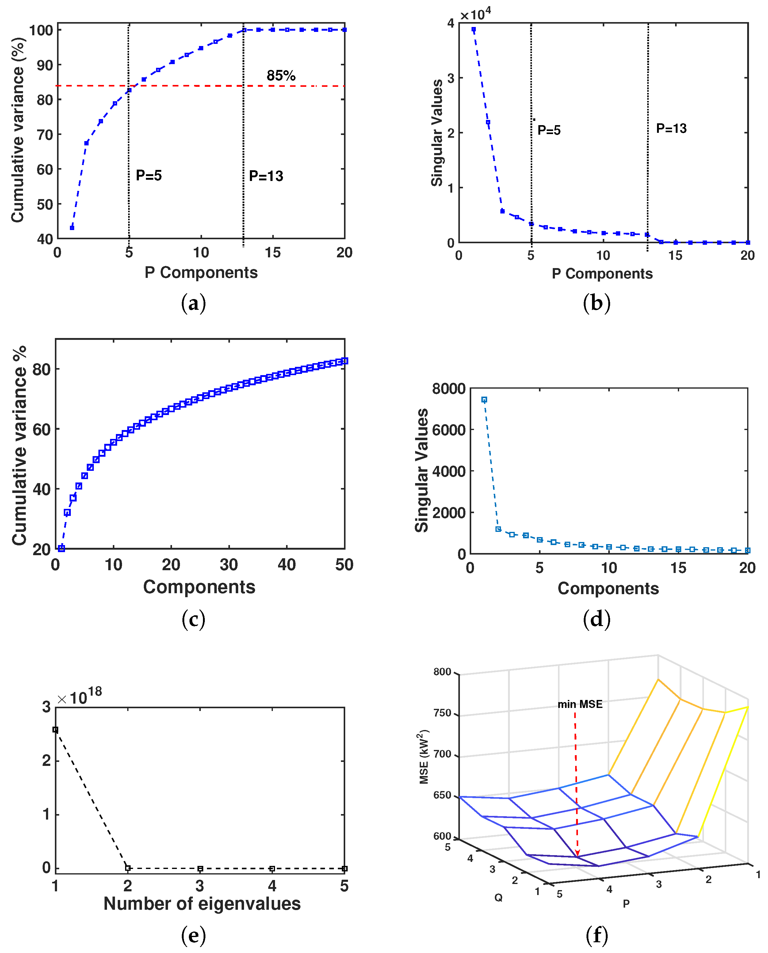
Both PCA and OPLS need to determine their suitable model order (i.e., the minimum number of components) to effectively compress the information while retaining the complexity of the data dynamics. In the PCA approach, we analyzed the dimensionality reduction in terms of the variance (eigenvalue) criterion. For the HUF case, Figure 2a depicts with a red dashed line the threshold to determine the P first principal components when considering 85% of the cumulative variance, as an operative and widely used rule of thumb. We selected P = 5 components according to this rule. Such a choice is confirmed in Figure 2b, where the energy of the original data contained by each component is also shown, although redundantly, for a better visualization. We also observe that almost all of the variance (close to 100%) accumulated at P = 13 components.
For the CEA case, the cumulative variance and the singular values are shown in Figure 2c,d, respectively. We can observe now different decomposition dynamics compared with the HUF case, given by a gradual variation with no clear cut-off point. This implies that a clear model order cannot be obtained and that the choice must be made on the basis of the relative relevance of the error versus the compression performance.
The model order selection in OPLS also requires validating the number of components to be included in terms of the eigenvalue profile. In Figure 2e, we observe that, for the HUF dataset, the first and second eigenvalues accumulated practically all the statistical energy from the OPLS projections, indicating that the required number of features from this model was Q = 2 . For the OPLS in the CEA case, we also selected Q = 2 as the number of principal components, considering that the relationship between the length of the data observation in years and the maximum number of eigenvalues was equal to 2. Given the number of available years and the necessity of prediction and model order selection, it was not possible to scrutinize larger model orders here.
For the HUF data, we have that P = 5 was a suitable order for PCA, whereas an order of Q = 2 was appropriate for OPLS. When designing the parameters for our ensemble (convex combination) algorithm, we needed not only to select the free parameter α (which dictates the weight of the convex combination), but also P and Q. To carry out this joint choice, a leave-one-out cross-validation (LOOCV) scheme and a grid search strategy based on a MSE criterion were performed. For LOOCV, we modified the partitions used to train and test the model; every year of the dataset was used as output, an observation was carried out from the training data. For the grid strategy, we searched for the coordinate in the hyperplane p q with the minimum MSE output. Figure 2f shows the results of a slice in the search process, where hyperparameters P = 4 and Q = 2 were obtained for the model with the minimum MSE.

4.2. Performance Results

Table 2 and Table 3 show the prediction performance using the metrics defined in Equations (11)–(14). For the HUF dataset, the results were consistent with the three methods tested. As expected, the ensemble algorithm obtained the best accuracy (i.e., lowest RMSE and MAPE ≤ 5%) with respect to the individual PCA and OPLS models. In Table 2, a negative value in PBIAS for the PCA method indicates the presence of overestimation. Differently, the PBIAS for the OPLS method was positive, revealing that the forecasted output underestimated the true values. We note that in this case, the PBIAS (≤ 1%) was also reduced for the ensemble algorithm.
For the HUF, the residual analysis in terms of its histograms is shown in Figure 3a, where the bias compensation effect is clearly seen from the mode (maximum peak) of the distributions. Additionally, it can be seen that all methods presented a marked asymmetry in their tails, with negative residual tails being markedly heavier and longer than positive residual tails.
Figure 4a–c boxplots the (error) residuals for the forecasted output in the HUF dataset for the three proposed methods. It can be observed that the PCA method tended to be residual-centered, except after March, when there was a trend of negative residuals dominating, whereas the OPLS method tended to have predominantly positive residuals between November and February. The use of the convex ensemble method yielded a “more centered” set of residuals. In all cases, two kinds of dynamics were revealed: one with lower variance (from October to May), and another with higher variance (from June to September), which was clearly consistent with the yearly seasonality. Figure 4d–f shows the Bland–Altman plots for the three methods. A Blant–Alman plot is a scatter-type representation in which the horizontal axis represents the measured load and the vertical axis represents its corresponding residual. For our dataset, this information showed that heteroscedasticity was indeed present, that is, the variance was not equally distributed along the load. For instance, lower loads consistently had a lower variance, whereas larger loads had an increased variance (and they were biased to negative residuals in all the models). It can be noted that extreme load peaks reduced the variance with respect to the intermediate values, which indicates that the models were more accurate when predicting the peak values.
In Figure 4g–i, residuals are shown for the CEA dataset. Similarly to the HUF dataset, there was a noticeable difference in the variance from June to September, compared to that of the months between October and May. On the other hand, the atypical residuals above the red dotted line were systematically present in the CEA data, while in the HUF case, such a presence was sporadic. This suggests that the model was biased, which was clearly confirmed by the Bland–Altman plots shown in Figure 4j–l. Heteroscedasticity was not so present, but instead, strongly biased residuals were observed, with a systematic trend of low (high) load amplitudes to be associated with negative (positive) residuals. The presence of this kind of bias in Bland–Altman plots often indicates that the model does not adequately capture the forecast dynamics, and, in this case, further analysis of the data and of the eigenvectors could provide useful insights on the model expression capabilities.

4.3. Results of Eigenvector Analysis

Both the PCA and OPLS methods identified eigenvectors whose profile and relevance were extremely useful to analyze the complexity patterns and the different dynamics of the forecasted load. The purpose of this section is to carry out a first analysis of those eigenvectors.
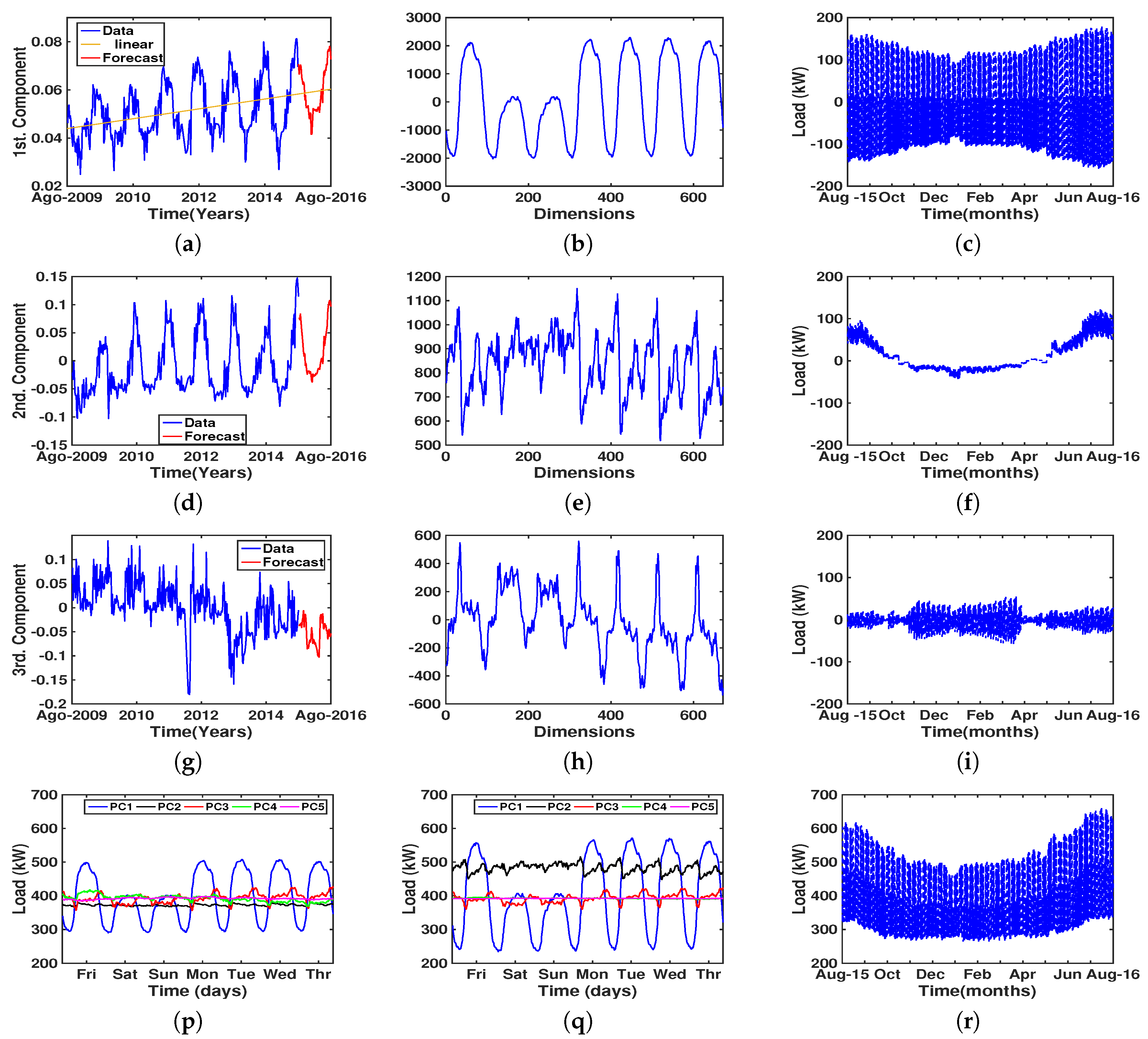
PCA Eigenvector Analysis for HUF. Figure 5 plots the time trajectories for the first three eigenvectors identified after applying PCA to the HUF dataset. Figure 5a shows the projection of the first component on the training data set, showing its annual linear trend by the yellow line superimposed on the load time series. The observed behavior confirms that the component was informative for prediction purposes and that the linear trend had to be accounted for. In red, we have depicted the one-year-ahead forecasted AR component, which followed nicely the pattern of the previous years (blue line). Figure 5b shows the first eigenvector, which clearly accounted for the weekly rhythm with a smooth representation, indicating that this component corresponded to an “average week”. We note that the load component was different on Saturdays and Sundays (second and third peaks) compared with the other days. Figure 5c shows that this pattern represented a smooth trend associated with the two previously identified periods with different residual dynamics but with a slow transition from one to the other as an envelope. Figure 5d,g shows the projections of the second and third components, as well as their AR predicted values, whereas Figure 5e,g represents their associated eigenvectors, which became peaked waveforms, indicating that they were acting as detail markers of the specific form of the average pattern given by the first component. We note that Figure 5f,i shows that their contribution was similarly linked to the two periods with different seasonal dynamics, but the second component showed a smooth behavior, whereas the third component was closer to an on–off switch behavior. To gain further insights, we chose two weeks from our dataset (one from summer and another from winter) and analyzed how strongly each of the different principal components was present in them. As seen in Figure 5p,q, they allowed us to better visualize and understand which component was contributing to an example week in the summer and to another example week in the winter.
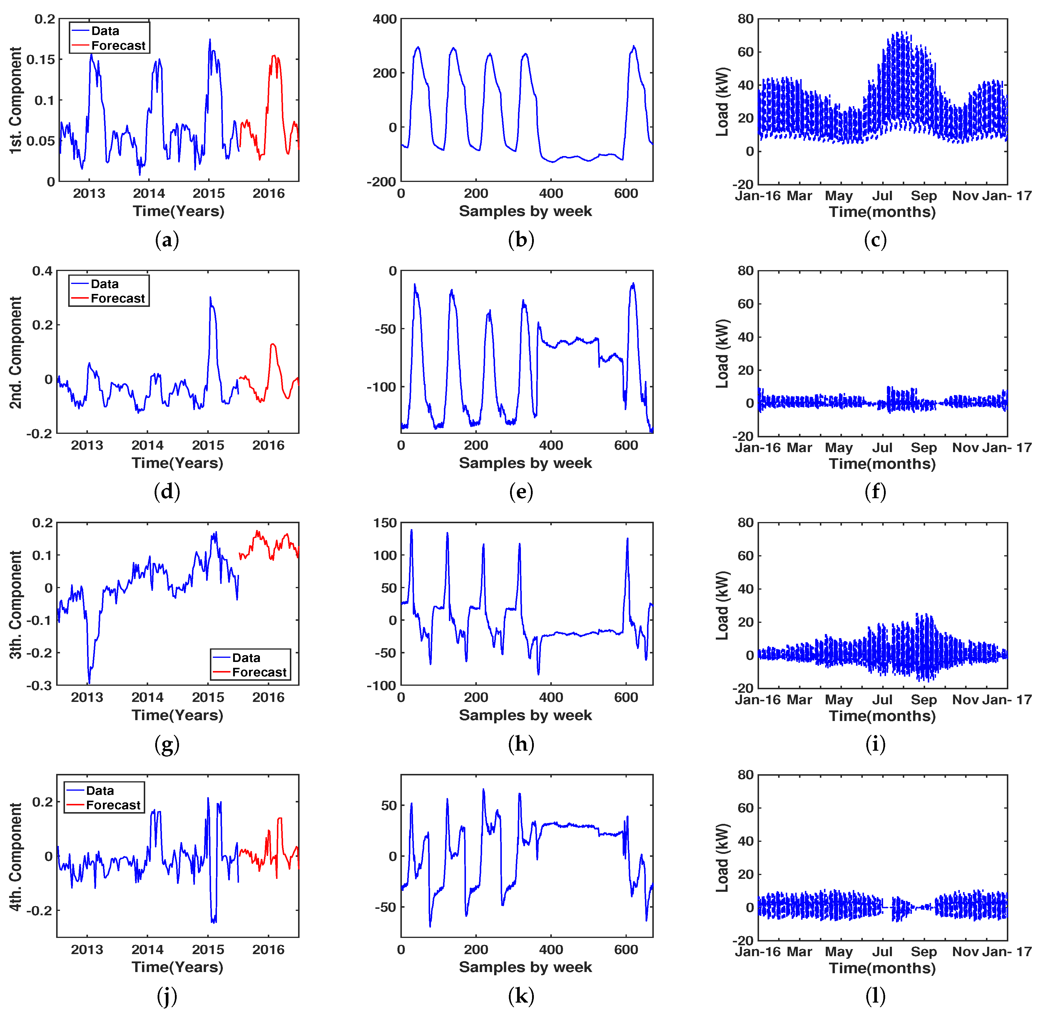
PCA Eigenvector Analysis for CEA. In Figure 6, we scrutinize the time plot of the first four components obtained after applying PCA to the CEA dataset. The first component again had a strongly seasonal variation in the coefficients (a), a smooth weekly pattern with different behavior during weekends (b), and two different dynamics behaviors for the partial estimation of the load (c). While the behavior of the first component was similar to that of the first component in the HUF dataset, a markedly different second component was observed. Being more specific, the coefficients (d) consisted of a seasonal component and a peak in 2015, which was partially predicted in 2016. A smooth eigenvector was observed, but with a flat level during the weekend, which pointed to a load increase, as opposed to the low-level load in the first eigenvector. We note that the third and fourth components were not so strongly periodic in terms of their annual coefficients. Additionally, their eigenvectors again accounted for peak details that included the form of small details when summed to the smooth first eigenvectors. However, a high- and a flat-load level could be seen in each of them during the weekends, which means that they were accounting for dynamics not present in the HUF dataset.
These results prompted further research into the historical management of the CEA. According to subsequent reports from the maintenance department of the CEA, the average temperature in the city in which the care center is located had been increasing during the previous years. As a result, during 2015, the air conditioning system was required to be on during the (summer) weekends; otherwise, it took Monday and Tuesday to recover habitability, particularly for patients. Moreover, during 2016, the situation became harder to manage at the beginning of every day, and the management also decided to maintain the air conditioning at some level during the summer months. This clearly represented a non-stationary situation that interacted with the otherwise simple and similar dynamics of the CEA. If the goal is to generalize this modeling technique to analyze and forecast energy loads in small healthcare buildings other than the CEA, different intervention methods could be used to handle non-stationary situations similar to that observed in this case.
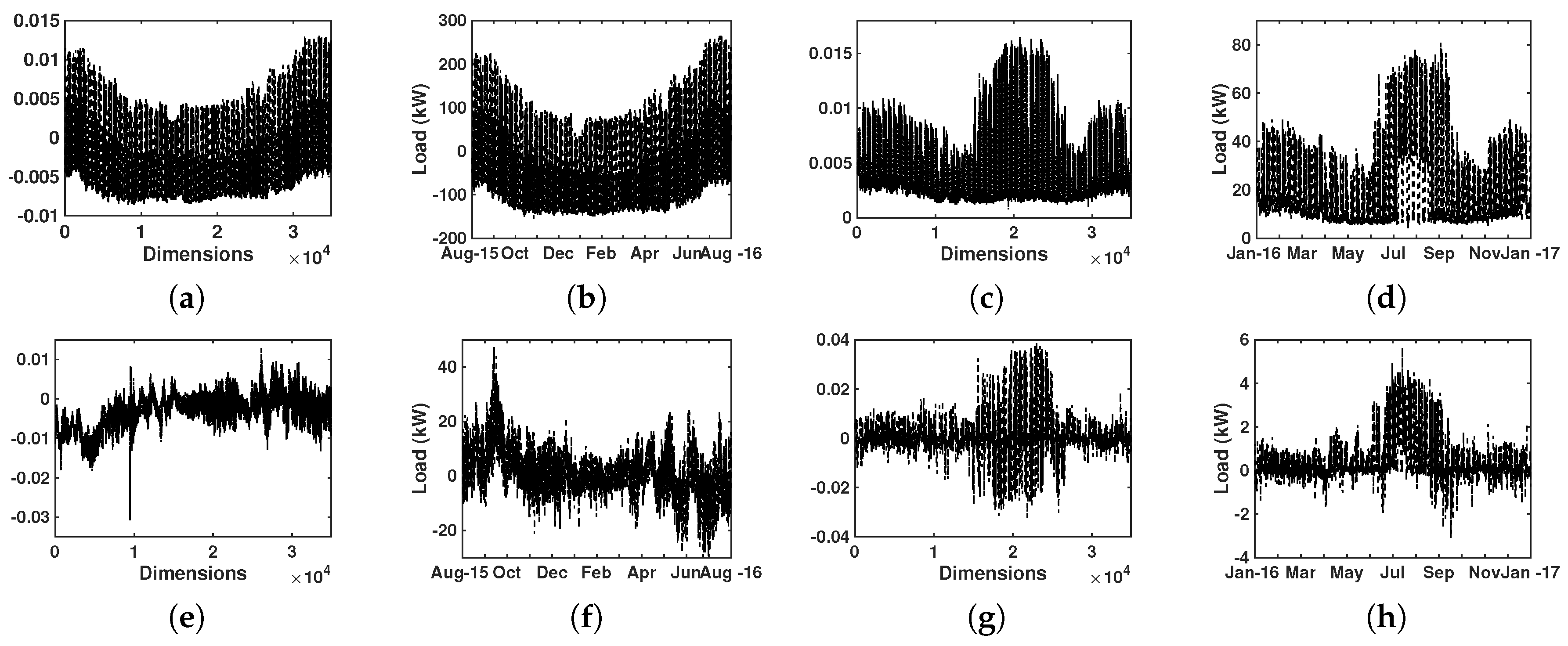
OPLS Eigenvector Analysis. Similarly to the PCA method, we analyzed the principal components of the OPLS models using the first eigenvectors and the data projection on them. As described before, the model order for OPLS was Q = 2 ; hence the two largest eigenvalues were identified and yielded their eigenvectors as the principal components of this supervised model. The interpretation of the results in the OPLS case was somewhat more challenging, as each year was provided as the sum of the two previous annual components. Nevertheless, in Figure 7, we have plotted the contours for the first and second eigenvectors, both for the HUF and for the CEA datasets, together with the projections on their corresponding load profiles. These played similar roles to those the eigenvectors and the signal projection coefficients played in the PCA decomposition.
The results for the HUF dataset revealed that the first component consisted again of smooth and repetitive variations, whereas the second gave the detail not only in terms of the weekly waveform but also for the yearly trend, with some fast transitions and peaks. This means that the expressive capacity of the supervised method allowed it to retain similar explanatory dynamics with just two components, which was advantageous compared with the non-supervised approach that required up to four components. Similar considerations could be made with the CEA model shown in the right panels. In both cases, a closer view into the eigenvectors and the projections showed that the first annual component exhibited a smooth long-term pattern, mixed with weekly and daily variations in both healthcare buildings, whereas the second component included the long-term transients mixed also with weekly and daily variations. For the HUF dataset, the long-term variations in this components also indicated the existence of two seasonal periods (increased and decreased consumption), which were present in both eigenvectors. It is also interesting to note that the increased variance during the summer period was only observed for the coefficients of the second projection but was not for those of the first projection. This contrasted with the CEA dataset, for which the existence of two seasonal periods was observed in both projection coefficients.
Overall, we observed that, while with some differences, the dynamics revealed when using OPLS were relatively similar to those revealed when using PCA. OPLS eigenvectors and coefficients could be seen as capturing the same information as PCA, but with a global description and a better confinement of similar variance in the first component. Nevertheless, the essentials of the dynamics captured by both approaches were strongly consistent.

5. Discussion

This paper has investigated the prediction of the energy consumption of healthcare customers using simple MVA methods. The reason for focusing our research on the customer side and selecting healthcare buildings as special customers was that healthcare services demand continuous and rhythmic energy and electricity use, which in most cases, does not have subsidies from the goverment entities. To our best knowledge, the literature review provides limited information about the analysis and forecasting of electrical loads with data provided by this special type of customer. As a consequence, and in order to meet the above requirements, our research led us to handle a large amount of data (i.e., high-dimensional data), which is the reason we explored the use of MVA methods for analysis and load forecasting.
In the load forecasting literature, a number of prediction methods have been reported and discussed [4,20,21]. Early works relied on well-known statistical methods, such as simple regression, multiple linear regression, and AR integrated moving-average modeling. Recently, the “intelligent methods” have become more relevant. These include artificial neural networks, fuzzy logic, support vector machines, or genetic algorithms, among others, and they have improved the accuracy of load forecasting [22,23,24]. These methods have some advantages, such as their ability of nonlinear approximation and self-learning or a higher adaptive capacity. While, for the particular case of healthcare buildings, these more advanced methods could be useful, the results in this paper indicate that their use should be further motivated. Indeed, the simple MVA methods presented here have not only shown that good prediction accuracy can be achieved, but also that the dynamics present in the analyzed datasets were not very complex.
This piece of research is part of a wider project that seeks the optimal design of the contracted power by the customers, where a yearly load profile is required (i.e., mid-term) [25]. Considering past (i.e., historical) and future (i.e., forecasted) profiles, the contracted power should be selected with accurately estimated information. Additionally, in terms of the target application, the forecasted output should meet another requirement, as far as that it should have high enough detail for keeping the same time resolution as the input data (i.e., sampling time interval of 15 min in our case). This implies the increase of both data dimensions and their cross-correlations.

6. Concluding Remarks

This paper has put forward several MVA methods to understand and predict the electrical load in two types of healthcare buildings. The dynamics of short- and middle-term predictions were analyzed by implementing unsupervised (OPLS), supervised (PCA), and ensemble (convex-combination) methods. The models were trained and adjusted by using historical datasets from 7 years for the HUF (2008–2015), a medium-to-large-sized hospital, and from 3 years for the CEA (2012–2015), a smaller care center. The predictive performance of the proposed models was evaluated by means of a dataset from the year 2016. By analyzing the accuracy of the forecasts in terms of the RMSE, MAPE, and PBIAS metrics, a satisfactory model prediction was obtained for the HUF dataset, achieving a one-year-ahead load profile with an intraday high level of resolution. For the CEA dataset, the analysis revealed an abrupt change in the average prediction error, which served to identify changes in the energy consumption patterns implemented by the managers of the building under study. Finally, the (compression) features generated by the proposed methods revealed insights and provided a detailed description of the energy consumption of the different health-building consumers. Interestingly, in both buildings, the dynamics observed exhibited a low complexity, which facilitated their prediction via linear models. When considered jointly, these findings constitute a solid starting point to identify the savings opportunities in the energy bill of the users at hand, which will be the subject of our future research.
References

Acknowledgments

Special thanks are given to Rafael Chillón and the staff of the HUF for their kind support in the data assembling. This work was partly supported by the research grants PRINCIPIAS, FINALE, KERMES and OMICRON (TEC2013-48439-C4-1-R, TEC2016-75161-C2-1-R, TEC2016-81900-REDT, and TEC2013-41604-R), by the Spanish Government, and by PRICAM (S2013/ICE-2933), from the Comunidad de Madrid, Spain.

Author Contributions

R.G.-O., L.M.L.-R., S.M.-R., and J.L.R.-Á. conceived and designed the experiments. R.G.-O., L.M.L.-R., and S.M.-R. performed the experiments. R.G.-O., S.M.-R., and J.L.R.-Á. organized and wrote the paper, and performed the analysis of the experimental results. R.G.-O. wrote the paper, and L.M.L.-R., S.M.-R., and A.G.M. contributed to writing and reviewing several sections of the manuscript. P.I.-C. elaborated on the hospital data structure. D.A.-A., A.G.M., and P.I.-C. collaborated with a multidisciplinary review.

Conflicts of Interest

The authors declare no conflict of interest.

References

  1. Soliman, S.A.H.; Al-Kandari, A.M. Electrical Load Forecasting: Modeling and Model Construction; Elsevier: Burlington, MA, USA, 2010; ISBN 978-0-12-381543-9. [Google Scholar]
  2. Abu-Shikhah, N.; Elkarmi, F.; Aloquili, O.M. Medium-term electric load forecasting using multivariable linear and non-linear regression. Smart Grid Renew. Energy 2011, 2, 126–135. [Google Scholar] [CrossRef]
  3. Ryu, S.; Noh, J.; Kim, H. Deep neural network based demand side short term load forecasting. Energies 2016, 10, 3. [Google Scholar] [CrossRef]
  4. Khuntia, S.R.; Rueda, J.L.; van der Meijden, M. Forecasting the load of electrical power systems in mid- and long-term horizons: A review. IET Gener. Transm. Distrib. 2016, 10, 3971–3977. [Google Scholar] [CrossRef]
  5. Hu, S.; Chen, J.; Chuah, Y. Energy cost and consumption in a large acute hospital. Int. J. Archit. Sci. 2004, 5, 11–19. [Google Scholar]
  6. Hong, T.; Shahidehpour, M. Load Forecasting Case Study; Department of Energy: Chicago, IL, USA, 2015.
  7. Alhurayess, S.; Darwish, M.K. Analysis of energy management in hospitals. In Proceedings of the 47th International Universities Power Engineering Conference (UPEC), London, UK, 4–7 September 2012; pp. 1–4. [Google Scholar] [CrossRef]
  8. Zhang, S.; Wang, D. Medium and long-term load forecasting based on PCA and BP neural network method. In Proceedings of the International Conference on Energy and Environment Technology, Guilin, China, 16–18 October 2009; pp. 389–391. [Google Scholar] [CrossRef]
  9. Tangirala, A.K. Principles of System Identification: Theory and Practice; CRC Press: Boca Raton, FL, USA, 2015; ISBN 978-1439895993. [Google Scholar]
  10. Hair, J.F.; Black, W.C.; Babin, B.J.; Anderson, R.E. Multivariate Data Analysis; Pearson: London, UK, 2009. [Google Scholar]
  11. Galbraith, J.W.; Green, C. Inference about trends in global temperature data. Clim. Chang. 1992, 22, 209–221. [Google Scholar] [CrossRef]
  12. Zheng, X.; Basher, R.E. Structural Time Series Models and Trend Detection in Global and Regional Temperature Series. J. Clim. 1999, 12, 2347–2358. [Google Scholar] [CrossRef]
  13. Huang, S.C.; Wang, N.Y.; Wu, T.K. High Dimensional Data Mining Systems by Kernel Orthonormalized Partial Least Square Analysis. Int. J. Futur. Comput. Commun. 2015, 4, 364–367. [Google Scholar] [CrossRef]
  14. Muñoz-Romero, S.; Arenas-García, J.; Gómez-Verdejo, V. Iterative orthonormalized partial least squares with sparsity constraints. In Proceedings of the IEEE International Conference on Acoustics, Speech and Signal Processing, Vancouver, BC, Canada, 26–31 May 2013; pp. 3387–3391. [Google Scholar] [CrossRef]
  15. Reinsel, G.C.; Velu, R.P. Multivariate Reduced-Rank Regression: Theory and Applications; Lecture Notes in Statistics; Springer: New York, NY, USA, 1998; ISBN 978-0-387-98601-2. [Google Scholar]
  16. Muñoz-Romero, S.; Arenas-García, J.; Gómez-Verdejo, V. Sparse and kernel OPLS feature extraction based on eigenvalue problem solving. Pattern Recognit. 2015, 48, 1797–1811. [Google Scholar] [CrossRef]
  17. Shawe-Taylor, J.; Cristianini, N. Kernel Methods for Pattern Analysis; Cambridge University Press: Cambridge, UK, 2004; ISBN 0521813972. [Google Scholar]
  18. Wu, Y.K.; Yang, W.W. Optimization of fuzzy relational equations with a linear convex combination of max-min and max-average compositions. In Proceedings of the IEEE International Conference on Industrial Engineering and Engineering Management, Singapore, 2–5 December 2007; pp. 832–836. [Google Scholar] [CrossRef]
  19. Jia, N.; Yokoyama, R.; Zhou, Y.; Gao, Z. A flexible long-term load forecasting approach based on new dynamic simulation theory—GSIM. Int. J. Electr. Power Energy Syst. 2001, 23, 549–556. [Google Scholar] [CrossRef]
  20. Chen, Y.H.; Hong, W.C.; Shen, W.; Huang, N.N. Electric load forecasting based on a least squares support vector machine with fuzzy time series and global harmony search algorithm. Energies 2016, 9, 70. [Google Scholar] [CrossRef]
  21. Hahn, H.; Meyer-Nieberg, S.; Pickl, S. Electric load forecasting methods: Tools for decision making. Eur. J. Oper. Res. 2009, 199, 902–907. [Google Scholar] [CrossRef]
  22. Bagnasco, A.; Saviozzi, M.; Silvestro, F.; Vinci, A.; Grillo, S.; Zennaro, E. Artificial neural network application to load forecasting in a large hospital facility. In Proceedings of the International Conference on Probabilistic Methods Applied to Power Systems (PMAPS), Durham, UK, 7–10 July 2014; pp. 1–6. [Google Scholar] [CrossRef]
  23. Stojanović, M.B.; Božić, M.M.; Stanković, M.M. Mid-term load forecasting using recursive time series prediction strategy with support vector machines. Facta Univ.-Ser. Electron. Energ. 2010, 23, 287–298. [Google Scholar] [CrossRef]
  24. Papaioannou, G.P.; Dikaiakos, C.; Dramountanis, A.; Papaioannou, P.G. Analysis and modeling for short-to medium-term load forecasting using a hybrid manifold learning principal component model and comparison with classical statistical models (SARIMAX, Exponential Smoothing) and artificial intelligence models (ANN, SVM): The case of Greek electricity market. Energies 2016, 9, 635. [Google Scholar] [CrossRef]
  25. Di Silvio, B.; Cesarotti, V.; Introna, V. Evaluation of electricity rates through characterization and forecasting of energy consumption: A case study of an Italian industrial eligible customer. Int. J. Energy Sect. Manag. 2007, 1, 390–412. [Google Scholar] [CrossRef]
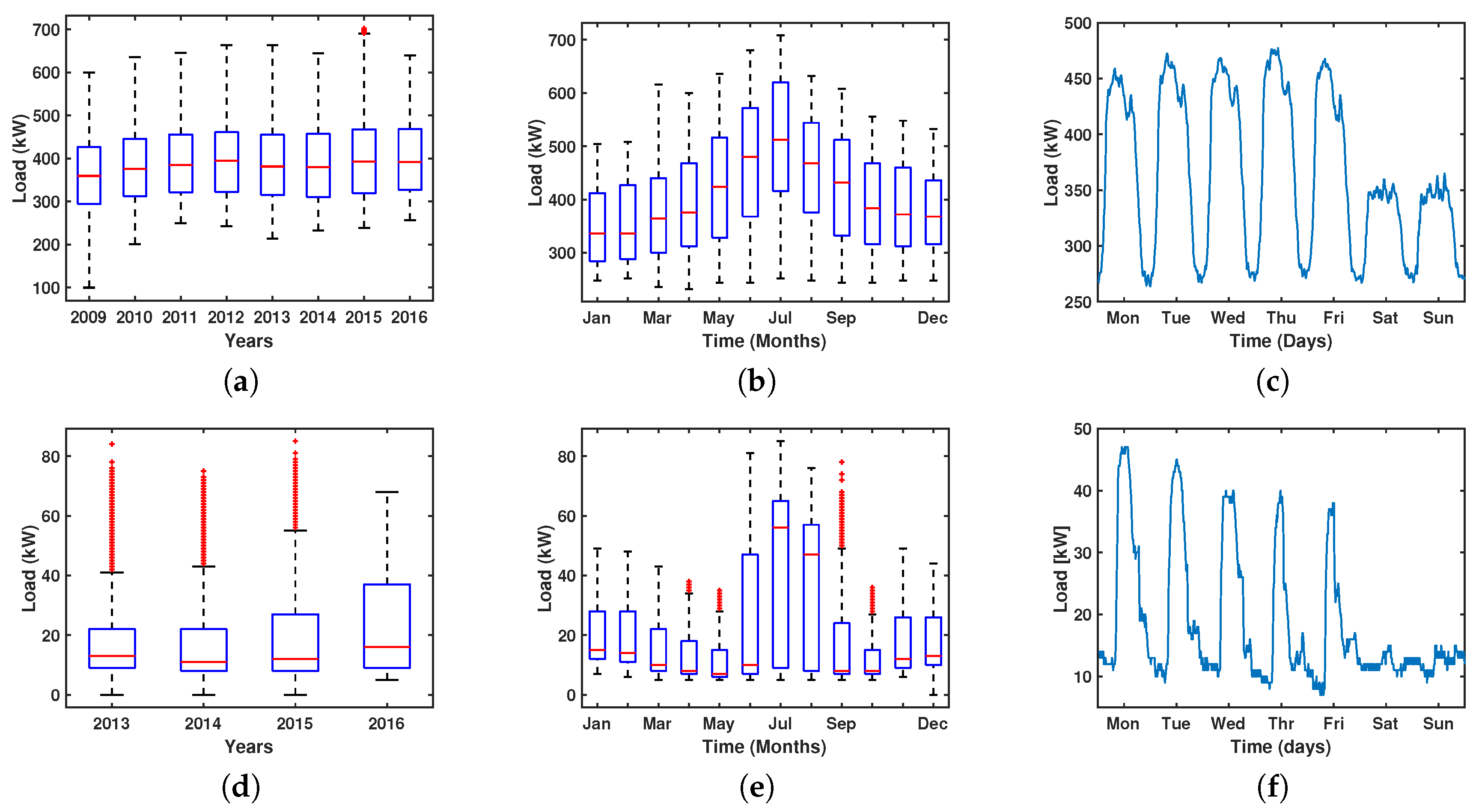
Figure 1. Database representation for the two healthcare buildings, Hospital Universitario de Fuenlabrada (HUF) (up) and Centro de Especialidades El Arroyo (CEA) (down): (a,d) electrical load and available data; (b,e) yearly load profile example; (c,f) weekly load profile example.
Energies 11 00493 g001
Figure 2. Model parameter selection procedures: (a) cumulative variance contribution rate for principal component analysis (PCA) model for Hospital Universitario de Fuenlabrada (HUF); (b) singular values from PCA model in HUF; (c,d) the same for Centro de Especialidades El Arroyo (CEA); (e) eigenvalue decomposition from orthonormal partial least squares (OPLS) in the HUF case; (f) grid search of hyperparameters in the HUF case.
Energies 11 00493 g002
Figure 3. Comparison of residual analysis distributions in terms of the histograms for the three analyzed methods: Hospital Universitario de Fuenlabrada (HUF) (a); Centro de Especialidades El Arroyo (CEA) (b,c). In the latter, two situations are considered: one when accounting for the complete test year (b), and another when excluding the summer (c), during which the management politics changed (see text for details).
Energies 11 00493 g003
Figure 4. Residual analysis for mid-term load forecasting for Hospital Universitario de Fuenlabrada (HUF) from September 2015 to August 2016 (a-f) and for Centro de Especialidades El Arroyo (CEA) from January 2016 to December 2016 (gl). Models for HUF, including residual plots for principal component analysis (PCA) (a), orthonormal partial least squares (OPLS) (b), and ensemble output (c), as well as Bland–Altman plots (d,e,f), in the same order; (gl) show the same representations with CEA data.
Energies 11 00493 g004
Figure 5. Principal component analysis (PCA) load prediction in Hospital Universitario de Fuenlabrada (HUF). For the the first, second, and third components, panels show the projection coefficient over the year (a,d,g), the eigenvector corresponding to the contribution of that component (b,e,h), and the yearly reconstructed partial load with that component (c,f,i). Panels (p,q) show two different reconstructed weeks in the two different periods, and (r) shows the reconstructed load with the first five components.
Energies 11 00493 g005
Figure 6. Principal component analysis (PCA) load prediction for Centro de Especialidades El Arroyo (CEA). For the first, second, third, and fourth components, panels show the projection of the coefficients over the year (a,d,g,j), the eigenvector corresponding to that component (b,e,h,k), and the yearly reconstructed partial load with that component (c,f,i,l).
Energies 11 00493 g006
Figure 7. Orthonormal partial least squares (OPLS) load prediction for Hospital Universitario de Fuenlabrada (HUF) (a,b,e,f) and for Centro de Especialidades El Arroyo (CEA) (c,d,g,h). For the HUF model, the first and second eigenvectors (a,e) are represented together with their coefficient projection on the test year (b,f). Similar plots for CEA are shown in terms of the two first eigenvectors (c,g) and their coefficient projections (d,h).
Energies 11 00493 g007
Table 1. Experiment settings.
SymbolDescriptionValue
T s Sampling time15 min
n H Number of samples by hour 60 / T s = 4
n d Day length of samples n H = 96
n w Week length of samples n d × 7 = 672
n y Year length of samples n w × 52 = 39 . 444
y d Year length in days364
y w Year length in weeks52
LDatabase length in years8 for Hospital of Fuenlabrada; 4 for Centro Especialidads el Arroyo
Table 2. Performance metric calculation.
DatasetData Base from Hospital (L = 7)CEA (L = 3)
Metric/MethodPCAOPLSENSPCAOPLSENS
RMSE (kW)28.9129.5326.7713.3313.1912.99
MAPE (%)5.065.964.8316.2115.1414.63
PBIAS (%)−2.871.38−0.747.585.816.69
Table 3. Performance in terms of training data size for Hospital Universitario de Fuenlabrada (HUF).
MetricMAPE (%)PBIAS (%)
Method/L (Years)7654376543
PCA5.064.935.005.085.11−2.87−1.67−0.84−0.35−3.16
OPLS5.966.116.015.9515.571.381.341.391.871.15
ENS4.835.135.285.324.85−0.74−0.160.270.75−1.00