Identifying the Optimal Offshore Areas for Wave Energy Converter Deployments in Taiwanese Waters Based on 12-Year Model Hindcasts


National Science and Technology Center for Disaster Reduction, New Taipei City 23143, Taiwan
*
Author to whom correspondence should be addressed.
Energies 2018, 11(3), 499; https://doi.org/10.3390/en11030499
Submission received: 8 January 2018
/
Revised: 29 January 2018
/
Accepted: 23 February 2018
/
Published: 27 February 2018
(This article belongs to the Special Issue Wave and Tidal Energy)
Abstract
:A 12-year sea-state hindcast for Taiwanese waters, covering the period from 2005 to 2016, was conducted using a fully coupled tide-surge-wave model. The hindcasts of significant wave height and peak period were employed to estimate the wave power resources in the waters surrounding Taiwan. Numerical simulations based on unstructured grids were converted to structured grids with a resolution of 25 × 25 km. The spatial distribution maps of offshore annual mean wave power were created for each year and for the 12-year period. Waters with higher wave power density were observed off the northern, northeastern, southeastern (south of Green Island and southeast of Lanyu) and southern coasts of Taiwan. Five energetic sea areas with spatial average annual total wave energy density of 60–90 MWh/m were selected for further analysis. The 25 × 25 km square grids were then downscaled to resolutions of 5 × 5 km, and five 5 × 5 km optimal areas were identified for wave energy converter deployments. The spatial average annual total wave energy yields at the five optimal areas (S1)–(S5) were estimated to be 64.3, 84.1, 84.5, 111.0 and 99.3 MWh/m, respectively. The prevailing wave directions for these five areas lie between east and northeast.
1. Introduction
Oceans cover over 70% of the Earth’s surface and represent a wealth of renewable energy resources [1]. Many potential candidates for ocean energy sources exist, including wave energy, tide energy, tidal current energy, thermal gradients and salinity gradients [2,3]. Of these, wave power is currently the most researched area; it represents the largest ocean energy resource and is the most widely distributed marine renewable energy around the world. Many methods of wave energy conversion have been developed to extract wave power from oceans. The overtopping/terminator type of wave energy converter (WEC) consists of two wave reflectors that collect overtopping water and convert the pressure head into power [4]. The raft-type WEC uses relative rotation around a hinge to drive an electrical generation system to convert wave energy to electricity [5]. Another approach involves a point-oscillating absorber type WEC, which utilizes relative translational motion in which the oscillating motion of the floater is converted into electricity by a power take off (PTO) system for the oscillating-body WEC. This type of WEC is widely used for offshore deployments [6]. The two-floater WEC also uses a PTO system to convert ocean wave-induced motion into electricity [7]. The attenuator type of WEC captures energy from the relative motions of two arms as waves pass.
The use of numerical models to assess ocean wave power has been widely adopted on both regional [8,9,10,11] and global scales [12,13,14,15] and has been implemented for several islands, including the Canary Islands, Madeira, and the Azores in the Atlantic Ocean [16,17,18,19], Hawaii and Taiwan in the Pacific Ocean [20,21,22,23], Fuerte Island in the Caribbean Sea [24], and Sardinia and Menorca in the Mediterranean Sea [25,26,27].
Hashemi and Neill [28] used a wave-tide coupled model called the Simulating WAves Nearshore-Regional Ocean Modeling System (SWAN-ROMS) to investigate wave energy resources in the seas along the northwest European shelf. Their results suggested that tidal impact is significant and that the contributions from the effects of tidal currents on wave power resources are greater than the contribution from variations in tide levels. The maximum current speeds of the Kuroshio in the eastern offshore sea of Taiwan range between 0.6 and 1.2 m/s [29]. Therefore, using a tide-surge-wave coupled model is essential for accurately assessing the distribution of wave power in Taiwanese waters.
There are substantial ocean energy resources around the Island of Taiwan. However, the statistical data issued from the Ministry of Economic Affairs, Taiwan, revealed that the annual total electricity generating capacity of Taiwan was 264.1 billion kWh in 2016, of which fuel-fired power accounted for 82% (216.56 billion kWh), nuclear power accounted for 12% (31.69 billion kWh), hydroelectric power accounted for 1.2% (3.17 billion kWh), and renewable power accounted for 4.8% (12.68 billion kWh). Regarding renewable energy, only wind power and solar power are currently utilized in Taiwan. However, exploitation of energy resources in the ocean is urgently needed in Taiwan because they are renewable and do not contribute to atmospheric pollution.
Assessments of optimal locations or hotspots for deploying wave energy converters in previous studies have usually been conducted by reporting the location of selected “points”. For instance, Morim et al. [30] evaluated the wave energy resources and optimal locations along the southeast coast of Australia, and Su et al. [23] assessed the distribution of wave power and hotspots for the surrounding waters of Taiwan. Although this method is quite straightforward, the possible energetic “sea area” where wave energy converters can be deployed is not definite. This is an important issue; wave energy converters should be placed in an “area” rather than at a “point”. In the present study, numerical simulations based on unstructured grids were converted to structured (square) grids to identify energetic “sea areas” using the gridding method available through ArcGIS software. The annual mean wave energy yields of the final optimal areas for WEC deployments were acquired by spatial averaging over 5 km square regions. The approach proposed in the present study is both innovative and helpful for assessing the most appropriate offshore sea areas in which to deploy wave energy converters in Taiwanese waters.
The primary objectives of the present study were as follows: (1) implement a tide-surge-wave fully coupled high-resolution model for Taiwanese waters; (2) validate the fully coupled model with available observations; (3) create spatial distribution maps for annual and 12-year-average wave power; (4) using the gridding method, identify the most energetic and optimal areas in the offshore seas of Taiwan for deploying wave energy converters; and (5) assess the annual total wave energy density and the dominant wave direction in each optimal area.
2. Methods and Data
2.1. Ocean Circulation Model
The sea surface elevations and currents of the waters surrounding Taiwan were simulated with the community ocean model Semi-implicit Cross-scale Hydroscience Integrated System Model (SCHISM). SCHISM is an upgraded and evolved version of the original Semi-implicit Eulerian-Lagrangian Finite-Element/volume (SELFE [31]) model that includes many enhancements and improvements such as a new extension to simulate large-scale eddying regimes and a seamless cross-scale capability ranging from creeks to oceans [32]. SCHISM and SELFE have been widely used to simulate the propagation of tsunami waves [33], to predict water quality and ecosystem dynamics [34,35,36], analyze oil spill diffusion and transport [37], generate flooding maps [38,39], evaluate the extent of inundation induced by extreme river flows, typhoons or hurricanes [40,41] and to estimate tidal-current power [42]. In Taiwanese waters, the surface circulation feature is highly similar to that on the bottom during the spring [43], and weak winter stratification is caused by vertical mixing [44]; therefore, a two-dimensional SCHISM model (SCHISM-2D) vertically integrated with the barotropic mode was employed in this study. The governing equations in the Cartesian coordinate system and two-dimensional form are as follows:
where η(x, y, t) is the free-surface elevation, H = η + h is the total water depth, h is the bathymetric depth, u(x, y, t) and ν(x, y, t) are the horizontal velocity components in the x, y direction, respectively, f is the Coriolis factor, g is the acceleration due to gravity, is the Earth’s tidal potential, α is the effective earth elasticity factor, ρ0 is the reference density of water, and PA(x, y, t) is the atmospheric pressure at the free surface. In Equations (2) and (3), τsx and τsy are the wind stress components in the x, y direction, respectively, and can be expressed as follows:
where Cs is the wind drag coefficient; ρa is the air density; and Wx, Wy are the wind-speed components 10 m above the sea surface in the x, y directions, respectively. Cs is often regarded as an increasing function of wind velocity; however, Powell et al. [45] suggested that Cs should be limited at high wind speeds. The formula to calculate Cs in SCHISM-2D is:
where W is the resultant wind speed at 10 m above the sea surface.
Here, τbx and τby are the bottom shear stress components in the x, y directions and are computed by the following formulas:
where Cd is the bottom drag coefficient, which can be parameterized as follows:
where n is the Manning coefficient, which was set to 0.025 in the model due to the lack of knowledge of the sea-bottom material type. However, the bottom drag coefficient Cd varies with H based on Equation (7).
Here, τrx and τry are the radiation stress components in the x, y directions, respectively, and can be computed following Longuet-Higgins and Stewart [46,47], as shown below:
where Sxx, Sxy and Syy are the wave radiation stress components and are represented according to Battjes [48]:
where N is the spectral wave action density, and the independent variables are the wave relative frequency, σ, and the wave direction, θ. Here, Cg and Cp are the wave group velocity and the wave phase velocity, respectively.
2.2. Spectral Wind Wave Model
A third-generation spectral wind wave model, Wind Wave Model III (WWM-III, 3.0, College of William & Mary, Williamsburg, VA, USA), was adopted to predict the significant wave heights (SWH) and wave peak period (Tp) in the coastal waters of Taiwan. The wave-action equation that governs WWM-III is given as:
where Cgx and Cgy are the wave group velocity components in the x, y direction, Cσ and Cθ are the propagation velocities in σ, θ space, respectively, and Stot is the sum of the source terms for wave variance, including non-linear interactions, wind growth and dissipation by white-capping, bottom friction and wave breaking. The bottom friction and peak enhancement factors are set to 0.067 and 3.3, respectively, based on the formulation of the Joint North Sea WAve Project (JONSWAP) [49]. WWM-III computes waves breaking in shallow-water areas using the method proposed by [50]. A constant wave-breaking coefficient of 0.78 was adopted. The maximum wave direction is 360°, which is discretized into 36 bins in WWM-III. The low- and high-frequency limits of the discrete wave frequency are 0.03 and 1.0 Hz, respectively and are also divided into 36 bins.
SCHISM-2D (College of William & Mary, Williamsburg, VA, USA) computes the depth-averaged current and water surface elevation and then passes the results to the wave model, WWM-III, which sends the radiation stress to SCHISM-2D after solving the wave action equation. More details about the model coupling procedures of SCHISM-WWM-III can be found in [51].
2.3. Meteorological and Boundary Conditions
The wind forcing data used to drive SCHISM-WWM-III were the wind field at 10 m above sea level and the sea level pressure produced by ERA-Interim, which were acquired from public datasets available from the European Center for Medium-Range Weather Forecasts (ECMWF). ERA-Interim is the latest global atmospheric reanalysis, which is normally updated monthly with a two-month delay [52]. The 10-m wind speed in the x, y components were extracted from the ERA-Interim reanalysis results with a temporal resolution of 6 h (four analysis fields per day, at 00:00, 06:00, 12:00 and 18:00 UTC) and a spatial resolution of 0.125° × 0.125° and converted to the unstructured grids of SCHISM-WWM-III using the Inverse Distance Weighting (IDW) method. The IDW formula is:
where pe(x, y) is the value to be estimated (the wind speed in SCHISM-WWM-III), pm(x, y) is the known value (the wind speed in ERA-Interim), and di represents the distances from the n data points to the point estimated n.
The wave boundary conditions of the regional SCHISM-WWM-III, including the significant wave height, the mean wave direction, the mean directional spreading, the peak frequency, and the zero down-crossing frequency, were obtained from a global WaveWatch III (WW III) model developed by the French Research Institute for Exploitation of the Sea (IFREMER) with a spatial resolution of 0.5° × 0.5° and a temporal resolution of 3 h. To obtain the tide boundary conditions, the harmonic constants of eight tidal constituents (M2, S2, N2, K2, K1, O1, P1, and Q1) were extracted from a regional inverse tidal model, China Seas & Indonesia 2016 [53], with a resolution of 1/30° and were set at each node on the open boundary to drive the model.
2.4. Estimation of Wave Power
The extractable wave power per unit of the wave crest length can be calculated through the spectral output of SCHISM-WWM-III and is given in kW per meter as shown below:
where S(σ, θ) is the directional wave variance density spectrum, ρ is the density of seawater, g is the acceleration due to gravity, and d is the water depth. The wave group velocity, cg(σ, θ), can be expressed as follows:
where κ = 2π/L is the number of waves, and L is the wave length. In deep water conditions (d > 0.5L) and cg(σ, θ) = g/4πσ, Then:
The spectral moments of order, n, are defined as follows:
The energy period Te and the significant wave height Hs in terms of spectral moment are as follows:
Therefore, Equation (11) can be simplified to:
If ρ is assumed to be 1025 kg/m3, Equation (18) becomes:
It has been suggested that Te is rarely specified and must be estimated from other variables, while the peak period Tp is often specified by measurements of sea states [23,49,50]. Te is equal to Tp when multiplied by a coefficient α:
in which α = 0.9 was adopted from the standard JONSWAP spectrum with a peak enhancement factor of γ = 3.3 [23,27,54,55]. Thus, the theoretical wave power at any point can be computed using the following expression:
The present study used Equation (15) to evaluate the wave power resources in Taiwanese waters, even when the deep-water hypothesis was not strictly satisfied [56].
Thus, the total annual wave energy per unit length can be generated for a given time interval and is calculated as follows:
where Δti is the temporal sampling interval; Δti = 1 h in the present study.
2.5. Model Configuration
The computational domain covers Taiwan in its entirety as well as its main offshore islands. The region covers the area from a longitude of 114° E to 130° E and a latitude of 19° N to 29° N, as shown in Figure 1a. Two gridded bathymetry datasets were employed in this study. One dataset consists of global data obtained from the General Bathymetric Chart of the Oceans (GEBCO) and has a resolution of 30 arc-seconds. It was generated by combining quality-controlled ship depth soundings with interpolations between the sounding points guided by satellite-derived gravitational data. The other dataset is local data provided by the Department of Land Administration, Ministry of the Interior in Taiwan, with a resolution of 200 m and is distributed over a longitude of only 100° E to 128° E and a latitude of 4° N to 29° N. The bathymetry data for the coupled model were produced by merging the GEBCO and local bathymetry datasets. The method for combining two bathymetry sets is to merge the values in some order of priority using Surface-water Modeling System (SMS) software. A priority must be adopted because data overlaps exist in the source datasets. In the present study, when overlap occurs, the GEBCO data points in a set are considered as lower priority than the local data points; thus, they are not included in the final merged set. When no overlap occurs, all data points are merged. This approach ensured the preservation of the high-resolution local data. Our modeling domain is composed of 278,630 triangular cells and 142,041 non-overlapping, unstructured grids. Coarse meshes with 30 km resolution were arranged on the open ocean boundaries, while fine meshes with 300 m resolution were used along the coastline of Taiwan and the small offshore islands (Figure 1b). After the unstructured grids were created, the final merged, gridded bathymetry dataset was interpolated to each node to represent the bottom elevations in the coupled model (Figure 1a) using the linear interpolation method in SMS software.
In the ocean circulation model, a time step of 120 s was used for the present unstructured-grid system with numerical stability. SCHISM and WWM-III exchange the computational results every five hydrodynamic time steps (i.e., the time step of WWM-III is 600 s).
3. Model Validation
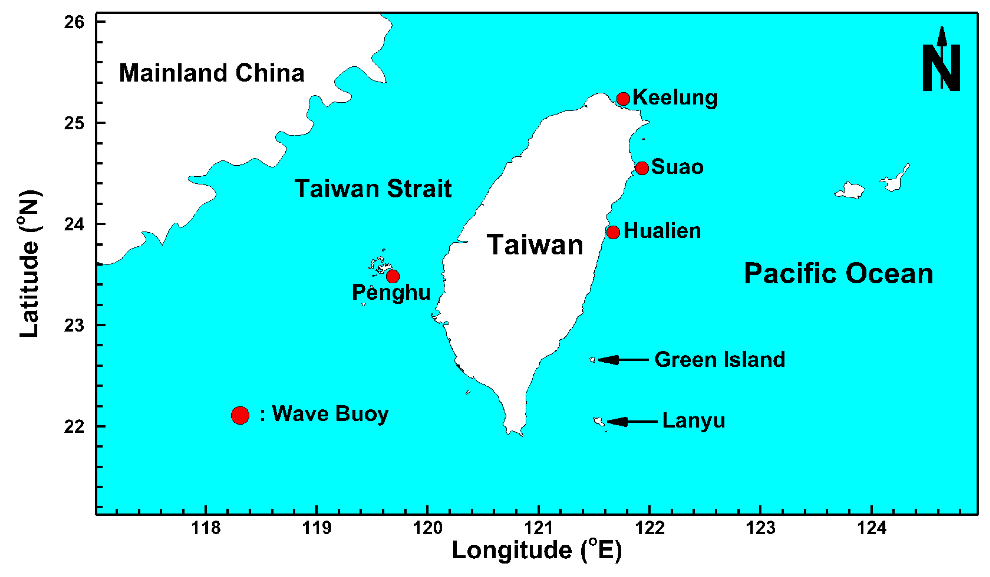
The observations adopted to validate SCHISM-WWM-III were measured significant wave heights (SWH) and peak periods (Tp) provided by the Harbor and Marine Technology Center (HMTC) in Taiwan at four buoys. The distribution map of these four wave buoys around Taiwanese waters is shown in Figure 2. The Keelung, Suao, and Hualien buoys are situated along the northeastern and eastern coast of Taiwan, while the Penghu buoy lies on the western coast of Taiwan (the Taiwan Strait). Figure 3 and Figure 4 present the comparisons of SWH (Figure 3) and Tp (Figure 4) between the model hindcasts and the measurements at the four buoys from 31 January 2016 to 30 December 2016. This period includes normal wind-generated waves (Tp), monsoon-induced waves (Tp) and the abnormal waves (Tp) caused by strong winds from Typhoon Nepartax (a severe typhoon, from 6 July 2016 to 9 July 2016), Typhoon Meranti (a severe typhoon, from 12 September 2016 to 15 September 2016) and Typhoon Megi (a moderate typhoon, from 25 September 2016 to 28 September 2016). The maximum SWH and Tp reached approximately 5.5 m and 14 s, 9.5 m and 16 s, 7.5 m and 15 s and 3.5 m and 13 s at the Keelung, Suao, Hualien, and Penghu buoys, respectively, due to the approach of Typhoon Megi. Peak SWH occurred at Keelung, Suao, and Hualien buoys on 28 September 2016, with a lag of almost one day at the Penghu buoy (as shown in Figure 3 and Figure 4). This result occurred because Typhoon Megi crossed Taiwan from east to west.
The statistical errors of the differences between the model hindcasts and the observations at the four wave buoys are also estimated. The correlation coefficients of the SWH and Tp are 0.86 and 0.74, 0.83 and 0.84, 0.87 and 0.83 and 0.80 and 0.73 for the Keelung, Suao, Hualien, and Penghu buoys, respectively. Even though the hindcasted SWH and Tp agree well with the measurements during both ordinary and extraordinary meteorological conditions, slight discrepancies still exist. It must be emphasized that the numerical wave models fail to capture Tp well, especially during normal meteorological conditions, for instance, April, May and June. The possible reasons include the nature of wave models. Some of the setup assumptions and numerical solutions within the models affect their accuracy [57]. In addition, the lower spatial and temporal resolutions of the wind field data from the ERA-Interim dataset affected model hindcasting, which is more sensitive to Tp. The adoption of higher spatial and temporal resolution wind data could improve the performance [58]. Yet a third reason for poor Tp hindcasts may be due to observational error. However, based on the model-data comparison, the hindcasts of SWH and Tp by SCHISM-WWM-III are relatively reliable and can be further applied to assess the distribution of wave power and wave energy in the waters surrounding Taiwan.
4. Results and Discussion
Sea-state hindcasts covering the period from 2005 to 2016 were conducted to estimate the wave power and wave energy output. Additionally, numerical simulations based on unstructured grids were converted to structured grids with a resolution of 25 × 25 km to locate the energetic sea areas.
4.1. Spatial Distribution of Annual Mean Significant Wave Height and Wave Power
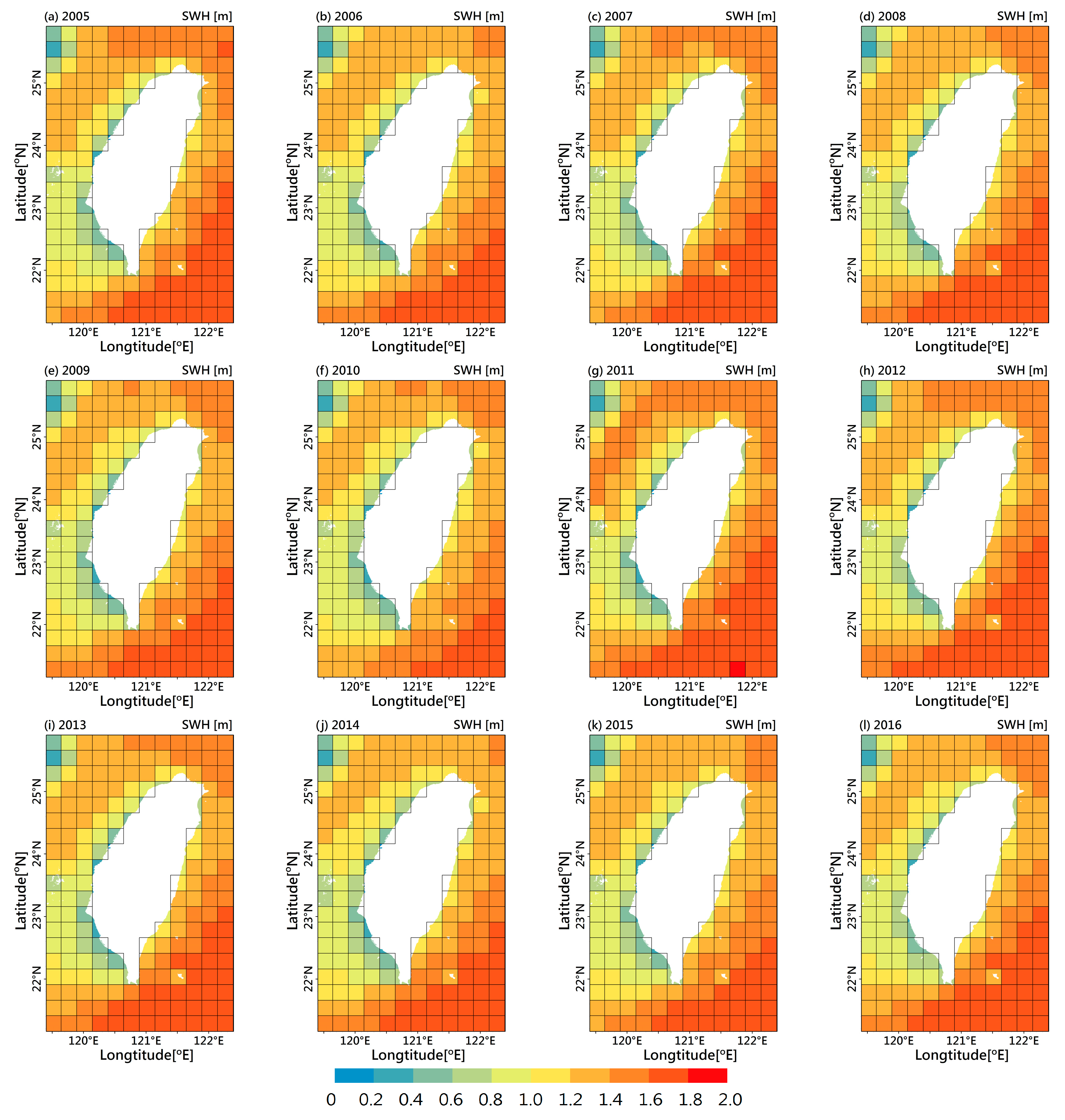
Figure 5 illustrates the spatial distribution of offshore annual mean SWH in Taiwanese waters for each year from 2005 to 2016 and shows highly similar patterns of mean SWH distribution. The mean SWH gradually increased from the nearshore region (shallower water) to the offshore areas (deeper water). This predictable phenomenon is due to the dissipation of SWH by depth effects [59]. The offshore sea areas with the higher SWH lie off the northeastern, eastern and southern coasts of Taiwan. The SWH values range from 1.2 m to 1.6 m along the northeastern coast and 1.4 m–1.8 m along the eastern and southern coasts. Figure 5 also shows that the mean SWH values are relatively low in the Taiwan Strait, ranging from only 0.6 m to 1.2 m. The spatial distribution of offshore SWH was averaged over 12 years (2005–2016) and is presented in Figure 6. The offshore sea areas southeast of Taiwan exhibit the highest mean SWH values, ranging from 1.2 m to 1.8 m. Although the prevalence of the strong northeast monsoon plays an important role in the higher SWH values, the deeper waters in this area also contribute to the SWH increases.
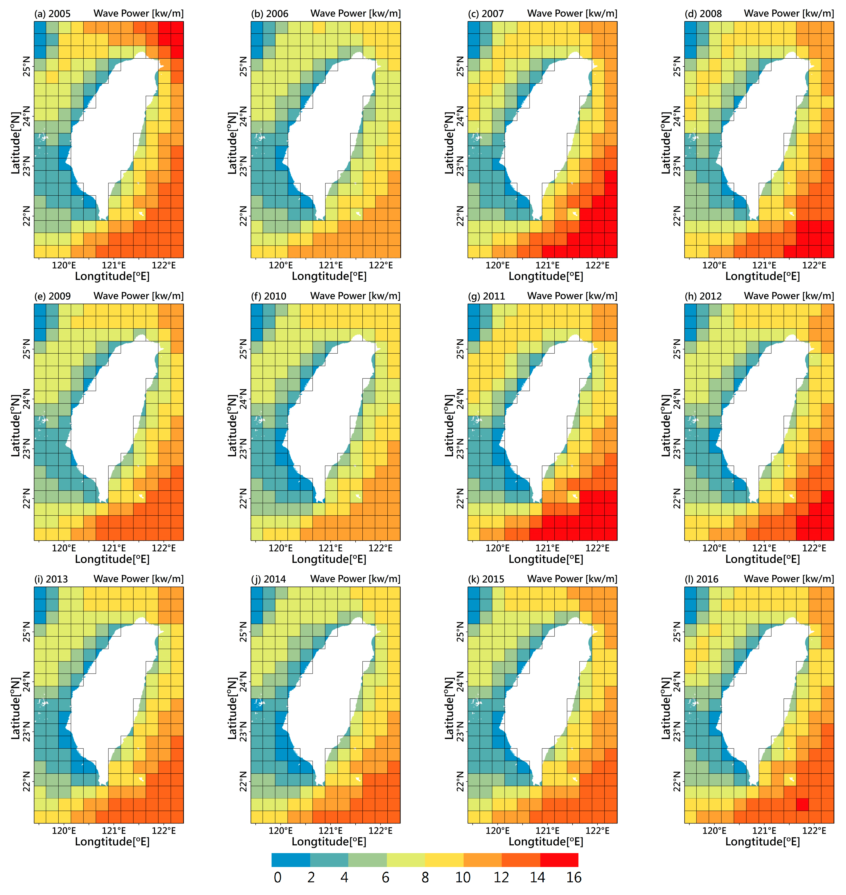
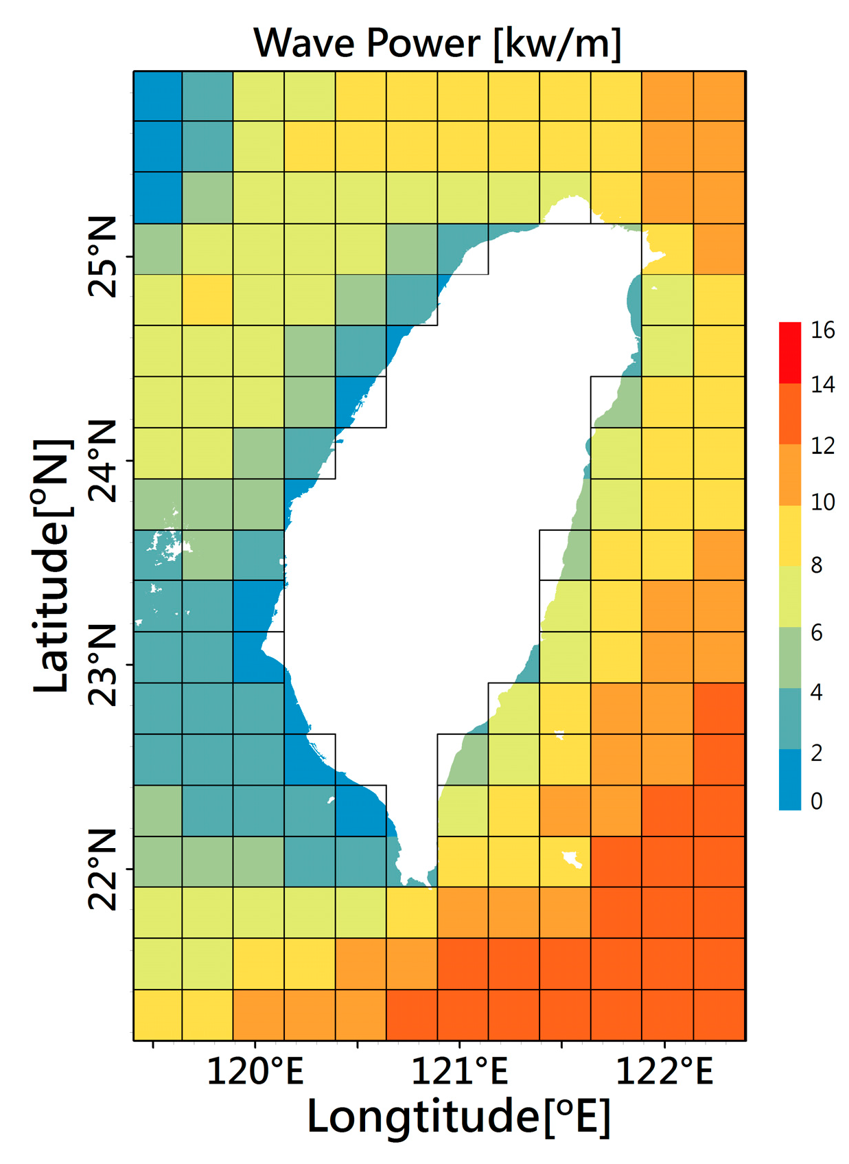
The SWH and Tp were output hourly from SCHISM-WWM-III to compute the wave power for each grid using Equation (21). Figure 7 demonstrates the spatial distribution of offshore annual mean wave power (in kW/m) in the waters surrounding Taiwan from 2005 to 2016. The more energetic sea areas are along the northeastern, eastern and southern coasts of Taiwan, and these locations are consistent with the distributions of the higher SWH. The mean wave power values were 6–12 kW/m for the northeastern coast and 8–16 kW/m for the eastern and the southern coast. The offshore wave power distribution for the 12-year annual mean is displayed in Figure 8. The most energetic areas are the eastern and the southeastern waters of Lanyu, with mean wave power values of 12–14 kW/m.
4.2. Identifying the Optimal Offshore Areas for Wave Energy Converter Deployment
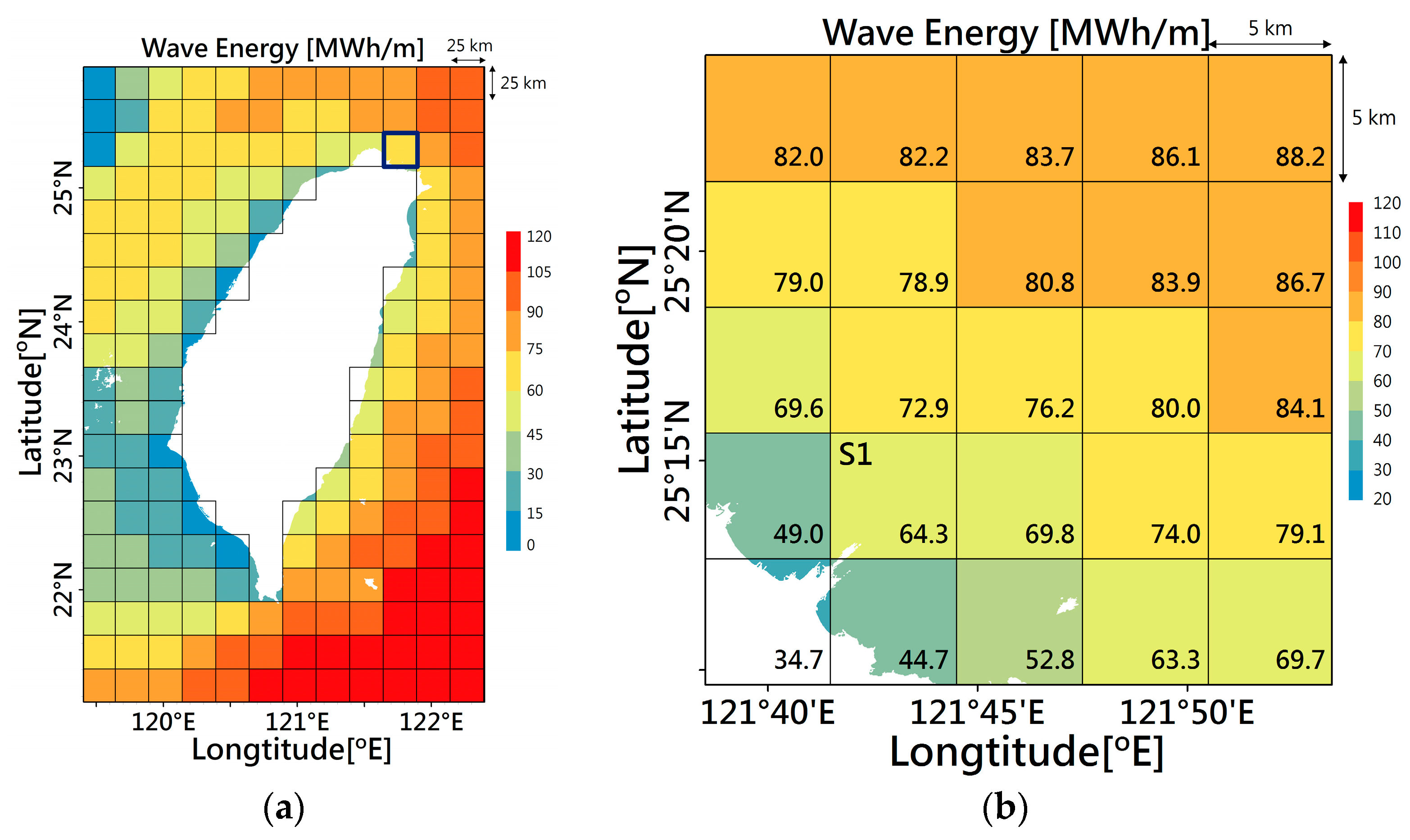
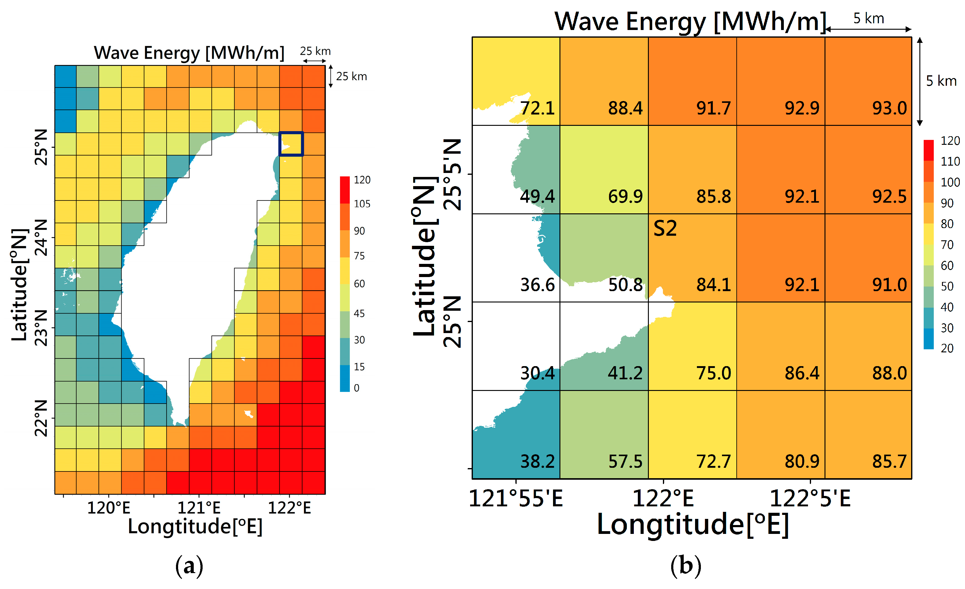
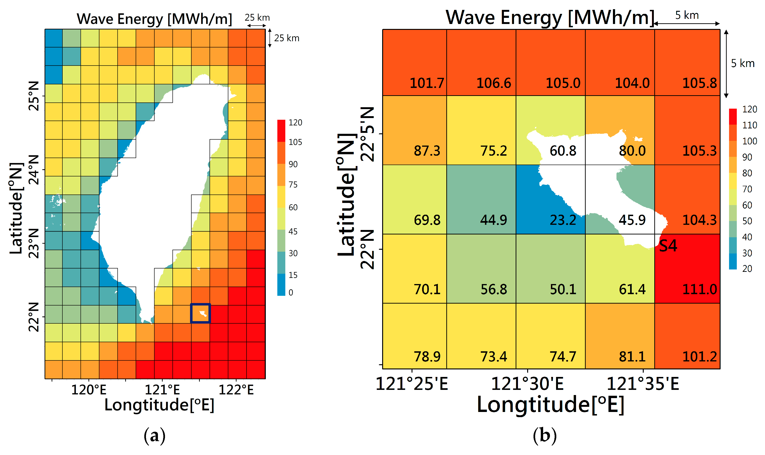
As shown in Figure 8, the offshore areas with the highest wave power density were observed off the northern, northeastern, southeastern (south of Green Island and southeast of Lanyu) and southern coasts of Taiwan. The annual total wave energy yields based on the 12-year average for each 25 × 25 km square grid were calculated by applying Equation (22) and are shown in Figure 9 (left panel). Even though higher wave energies exist in several sea areas, especially in the southeast (105–120 kW/m), the distance between coast and wave energy converter (WEC) should also be considered because of the cabling costs [19]. The five 25 × 25 km energetic sea areas marked with deep blue lines, with spatial average annual total wave energy density of 60–90 kW/m were selected for further analysis (as shown in the left panel of Figure 9, Figure 10, Figure 11, Figure 12 and Figure 13). The selected 25 × 25 km grid for the northern coast of Taiwan was downscaled to a resolution of 5 × 5 km. A total of 25 square grids are exhibited in the right panel of Figure 9. The grids are within 5 km of the coasts, have higher wave energies and were determined to be optimal areas for WEC deployments (see S1 in the right panel of Figure 9). The same approach was adopted to select an optimal area for the northeastern coast of Taiwan (S2 in the right panel of Figure 10), for the southern coast of Green Island (S3 in the right panel of Figure 11), for the southeastern coast of Lanyu (S4 in the right panel of Figure 12) and for the southern coast of Taiwan (S5 in the right panel of Figure 13). The spatial average (average over a square of 5 × 5 km) annual total wave energy densities are estimated to be 64.3, 84.1, 84.5, 111.0 and 99.3 MWh/m at S1, S2, S3, S4 and S5, respectively. The central longitudes, latitudes, and average water depths for these five optimal areas are listed in Table 1. In other words, the sea areas within 2.5 km of the central coordinate (as listed in Table 1) are considered to be appropriate sites for WEC deployments.
Tsai et al. [21] utilized the SWAN (Simulating WAves Nearshore) driven by NECP (National Centers for Environmental Prediction) global reanalysis wind field to hindcast waves and periods around Taiwanese waters. They revealed that higher significant wave heights were found near Lanyu. Chiu et al. [22] analyzed the temporal and spatial characteristics of wave power density in the coastal areas of Taiwan wave parameter hindcasts (significant wave height and period) based on the TaiCOMS model and observational data. Their results also indicated that the maximum annual mean wave power was found in Lanyu. Su et al. [23] employed the WWM-III model to assess the distribution of wave power in the waters surrounding Taiwan and suggested that the most energetic sea area is southeast of Lanyu. Thus, our results are consistent with those of previous studies.
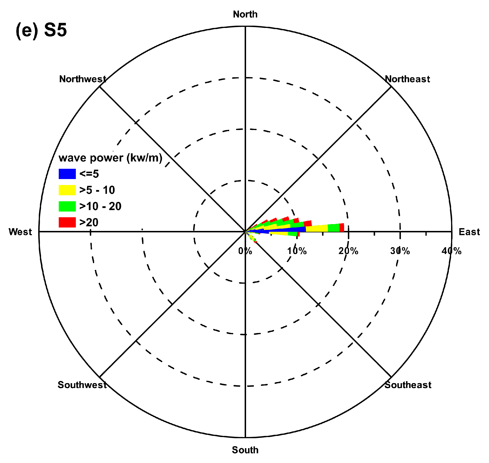
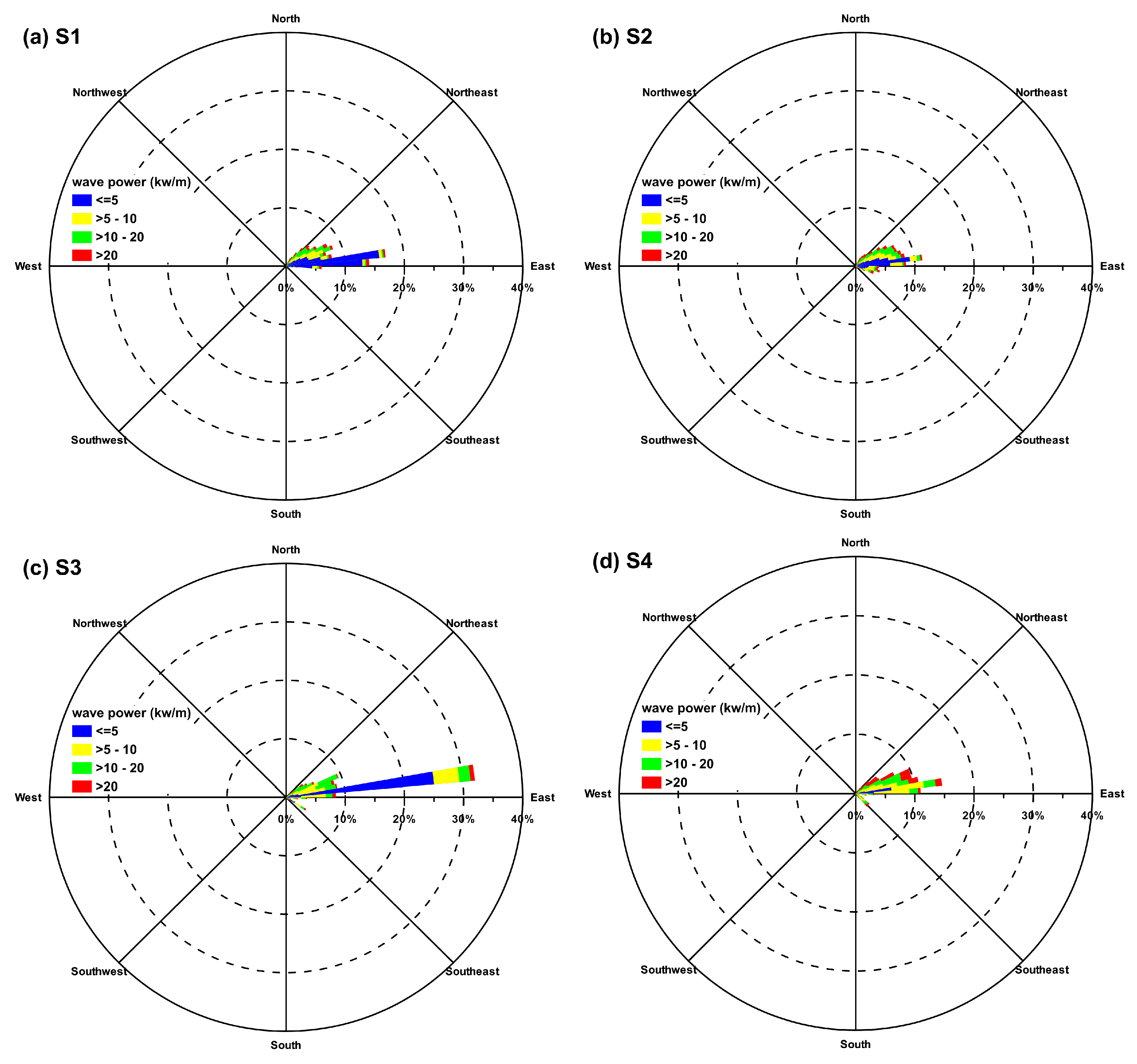
Wave direction is another important parameter that should be considered in WEC placements [60]. This is particularly true for attenuator-type and terminator-type Weeks: attenuators should be parallel to the predominant wave direction while the principal axis of terminator devices should be perpendicular to the predominant wave direction [61]. Point absorbers are buoy-type WECs that harvest incoming wave energy from all directions, however, arrays of this type of WEC can be sensitive to wave direction when they are deployed in offshore regions [6]. Figure 14 shows wave rose plots for the 12-year average at the centers of S1, S2, S3, S4 and S5. The dominant wave directions for these five optimal areas lie between east and northeast.
4.3. Discussion
In many coastal areas, nearshore regions have been considered to be the ideal locations for deploying wave energy converters due to their lower costs. However, by comparing wave lengths to wave energy conversion, the nearshore areas can be regarded as shallow-water areas. The effect of water depth on wave propagation is significant and cannot be neglected for wave energy assessment in shallow-water regions [62]. However, the effects of water depths are typically ignored because studies usually employ the formulas for deep-water waves. This simplification may underestimate the wave energy in finite water depths. Sheng and Li [63] conducted wave power assessment at a water depth of 50 m using the deep-water formula and the proposed method in their study and compared the results to the actual values. They found that the deep-water formula underestimated the annual mean wave power by up to 10.18% at the studied finite water depth (50 m). However, when the water depth modification factor (Ch) was considered, the underestimation of the annual mean wave power fell to 1.47%. Their results suggested that a modification of the deep-water formula is necessary to accurately assess wave power, especially in cases that involve finite water depth effects. Additionally, tide levels and wind intensity may influence the wave characteristics in shallow-water locations [64]. These effects are considered in our tide-surge-wave fully coupled model.
Additional uncertainties in wave power density assessments might be introduced by using a deep-water assumption (Equations (14)–(22)). However, this assumption causes obvious errors only in shallow water areas (i.e., those with water depths <0.5 × wavelength) [65]. The more energetic sea areas such as S1–S5 are located in the northern, eastern and southern offshore waters of Taiwan and can be regarded as deep-water areas. Therefore, the uncertainty of wave power density using Equation (21) can be ignored.
Guillou [66] employed SWAN (Simulating Waves Nearshore model) and TOAWAC (TELEMAC-based Operational Model Addressing Wave Action Computation) to evaluate wave power for the Iroise Sea. The results revealed that SWAN calculates a 15% lower mean wave power than does TOAWAC in offshore waters. Therefore, inter-model comparisons of wave power computation will be performed for Taiwanese waters in the near future.
The wind field data with a temporal resolution of 6 h and a spatial resolution of 0.125° by 0.125° from the ERA-interim dataset seems too low to accurately force a tide-surge-wave coupled model, although it is convenient for providing meteorological boundary conditions and producing an acceptable sea-state hindcast. Consequently, a three-layer nested WRF (Weather Research and Forecast, [67]) model with a temporal resolution of 1 h and a spatial resolution of 45 × 45 km for domain 1, 15 × 15 km for domain 2 and 5 × 5 km for domain 3 will be considered in the future as an alternative source of meteorological information to produce more accurate wave power estimations.
5. Conclusions
A tide-surge-wave fully coupled model based on an unstructured grid system, SCHISM-WWM-III, was implemented to simulate the sea states in the waters surrounding Taiwan. The wind field 10 m above sea level from the ERA-Interim reanalysis data and harmonic constants of eight tidal constituents extracted from a regional inverse tidal model were used to drive SCHISM-WWM-III. The fully coupled model was verified against available significant wave height and peak period measurements. Twelve-year model hindcasts for 2005–2016 were conducted to evaluate the spatial distributions of wave power and wave energy and to determine the most energetic areas in the offshore seas of Taiwan. Numerical simulations with unstructured grids were converted to 25 × 25 km structured grids to identify the most energetic sea areas. An offshore wave power and wave energy distribution map was created for the 12-year annual mean. Five 25 × 25 km energetic sea areas with spatial average annual total wave energy densities of 60–90 kW/m were selected and subsequently downscaled to resolutions of 5 × 5 km. The 5 × 5 km grids are within 5 km of the coasts and have higher wave energies and were determined to be optimal areas for WEC deployments. Five 5 × 5 km square areas off the northern, northeastern and southern coasts of Taiwan (S1, S2 and S5), the southern coast of Green Island (S3) and the southeastern coast of Lanyu (S4) were selected as the optimal areas for WEC deployments. The spatial average annual total wave energy densities are estimated to be 64.3, 84.1, 84.5, 111.0 and 99.3 MWh/m for the areas S1, S2, S3, S4 and S5, respectively. The dominant wave directions for these five optimal areas lie between east and northeast.
Acknowledgments
This research was supported by the Ministry of Science and Technology (MOST), Taiwan, grant Nos. MOST 106-2625-M-865-001. The authors would like to thank the Harbor and Marine Technology Center, Taiwan, for providing the observational data and Joseph Zhang at the Virginia Institute of Marine Science, College of William & Mary, and Aron Roland at the Institute for Hydraulic and Water Resources Engineering, Technische Universität Darmstadt, for kindly sharing their experiences concerning the use of the numerical model.
Author Contributions
Hung-Ju Shih, Chih-Hsin Chang, Lee-Yaw Lin and Wei-Bo Chen conceived the study, and Wei-Bo Chen performed the model simulations. The final manuscript has been read and approved by all the authors.
Conflicts of Interest
The authors declare no conflict of interest.
References
- U.S. National Renewable Energy Laboratory. Ocean Energy Technology Overview; U.S. Department of Energy Federal Energy Management Program; U.S. National Renewable Energy Laboratory: Lakewood, CO, USA, 2009.
- Defne, Z.; Hass, K.A.; Fritz, H.M. Numerical modeling of tidal currents and the effects of power extraction on estuarine hydrodynamics along the Georgia coast, USA. Renew. Energy 2011, 36, 3461–3471. [Google Scholar] [CrossRef]
- Lewis, M.J.; Angeloudis, A.; Robins, P.E.; Evans, P.S.; Neill, S.P. Influence of storm surge on tidal range energy. Energy 2017, 122, 25–36. [Google Scholar] [CrossRef]
- Kofoed, J.P.; Frigaard, P.; Friis-Madsen, E.; Sørensen, H.C. Prototype testing of the wave energy converter wave dragon. Renew. Energy 2006, 31, 181–189. [Google Scholar] [CrossRef]
- Zheng, S.M.; Zhang, Y.H.; Zhang, Y.L.; Sheng, W.A. Numerical study on the dynamics of a two-raft wave energy conversion device. J. Fluids Struct. 2015, 58, 271–290. [Google Scholar] [CrossRef]
- Zhang, X.; Yang, J. Power capture performance of an oscillating-body WEC with nonlinear snap through PTO systems in irregular waves. Appl. Ocean Res. 2015, 52, 261–273. [Google Scholar] [CrossRef]
- Zhang, X.; Lu, D.; Guo, F.; Gao, Y.; Sun, Y. The maximum wave energy conversion by two interconnected floaters: Effects of structural flexibility. Appl. Ocean Res. 2018, 71, 34–47. [Google Scholar] [CrossRef]
- Zhou, G.; Huang, J.; Zhang, G. Elevation of the wave energy conditions along the coastal waters of Beibu Gulf, China. Energy 2015, 85, 449–457. [Google Scholar] [CrossRef]
- Bento, R.A.; Martinho, P.; Soares, C.G. Numerical modelling of the wave energy in Galway Bay. Renew. Energy 2015, 78, 457–466. [Google Scholar] [CrossRef]
- Mirzaei, A.; Tangang, F.; Juneng, L. Wave energy potential assessment in the central and southern regions of the South China Sea. Renew. Energy 2015, 80, 454–470. [Google Scholar] [CrossRef]
- Akpmar, A.; Bingolbali, B.; Van Vledder, G.P. Long-term analysis of wave power potential in the Black Sea, Based on 31-year SWAN simulations. Ocean Eng. 2017, 13, 482–497. [Google Scholar] [CrossRef]
- Mork, G.; Barstow, S.; Kabuth, A.; Pontes, M.T. Assessing the global wave energy potential. In Proceedings of the ASME 2010 29th International Conference on Ocean, Offshore and Arctic Engineering, Shanghai, China, 6–11 June 2010; pp. 447–454. [Google Scholar] [CrossRef]
- Arinaga, R.A.; Cheung, K.F. Atlas of global wave energy from 10 years of reanalysis and hindcast data. Renew. Energy 2012, 39, 49–64. [Google Scholar] [CrossRef]
- Gunn, K.; Stock-Williams, C. Quantifying the global wave power resource. Renew. Energy 2012, 44, 296–304. [Google Scholar] [CrossRef]
- Reguero, B.G.; Losada, I.J.; Mendez, F.J. A global wave power resource and its seasonal, interannual and long-term variability. Appl. Energy 2015, 148, 366–380. [Google Scholar] [CrossRef]
- Iglesias, G.; Carballo, R. Wave power for La Isla Bonita. Energy 2010, 35, 513–521. [Google Scholar] [CrossRef]
- Iglesias, G.; Carballo, R. Wave resource in El Hiero—An island towards energy selfe-suficiency. Renew. Energy 2011, 36, 689–698. [Google Scholar] [CrossRef]
- Sierra, J.P.; Gonzale-Marco, D.; Sospedra, J.; Gironella, X.; Moss, A.; Sanchez-Arcilla, A. Wave energy resource assessment in Lanzarote (Spain). Renew. Energy 2013, 55, 480–489. [Google Scholar] [CrossRef]
- Goncalves, M.; Martinho, P.; Soares, C.G. Assessment of wave energy in the Canary Islands. Renew. Energy 2013, 68, 774–784. [Google Scholar] [CrossRef]
- Stopa, J.E.; Cheung, K.F.; Chen, Y.-L. Assessment of wave energy resources in Hawaii. Renew. Energy 2011, 36, 554–567. [Google Scholar] [CrossRef]
- Tsai, C.P.; Hwang, C.H.; Chuen, C.; Cheng, H.Y. Study on the wave climate variation to the renewable wave energy assessment. Renew. Energy 2012, 38, 50–60. [Google Scholar]
- Chiu, F.-C.; Huang, W.-Y.; Tiao, W.-C. The spatial and temporal characteristics of the wave energy resources around Taiwan. Renew. Energy 2013, 52, 218–221. [Google Scholar] [CrossRef]
- Su, W.-R.; Chen, H.; Chen, W.-B.; Chang, C.-H.; Lin, L.-Y.; Jang, J.-H.; Yu, Y.-C. Numerical investigation of wave energy resources and hotspots in the surrounding waters of Taiwan. Renew. Energy 2018, 118, 814–824. [Google Scholar] [CrossRef]
- Ortega, S.; Osorio, A.F.; Agudelo, P. Estimation of the wave power resource in the Caribbean Sea in areas with scarce instrumentation. Case study: Isla Fuerte, Colombia. Renew. Energy 2013, 57, 240–248. [Google Scholar] [CrossRef]
- Vicinanza, D.; Contestabile, P.; Ferrante, V. Wave energy potential in the northwest of Sardinia (Italy). Renew. Energy 2013, 50, 506–521. [Google Scholar] [CrossRef]
- Sierra, J.P.; Moss, A.; Gonzale-Marco, D. Wave energy resource assessment in Menorca (Spain). Renew. Energy 2014, 71, 51–60. [Google Scholar] [CrossRef]
- Sierra, J.P.; Casas-Prat, M.; Campins, E. Impact of climate change on wave energy resource: The case of Menorca (Spain). Renew. Energy 2017, 101, 275–285. [Google Scholar] [CrossRef]
- Hashemi, M.R.; Neill, S.P. The role of tides in shelf-scale simulations of the wave energy resource. Renew. Energy 2014, 69, 300–310. [Google Scholar] [CrossRef]
- Hsin, Y.C.; Wu, C.R.; Shaw, P.T. Spatial and temporal variations of the Kuroshio east of Taiwan, 1982–2005: A numerical study. J. Geophys. Res. 2008, 113, C04002. [Google Scholar] [CrossRef]
- Morim, J.; Cartwright, N.; Etemad-Shahidi, A.; Strauss, D.; Hemer, M. Wave energy resource assessment along the Southeast coast of Australia on the basis of a 31-year hindcast. Appl. Energy 2016, 184, 276–297. [Google Scholar] [CrossRef]
- Zhang, Y.J.; Baptista, A.M. SELFE: A semi-implicit Eulerian-Lagrangian finite-element model for cross-scale ocean circulation. Ocean Model. 2008, 21, 71–96. [Google Scholar] [CrossRef]
- Zhang, Y.; Ye, F.; Stanev, E.V.; Grashorn, S. Seamless cross-scale modelling with SCHISM. Ocean Model. 2016, 102, 64–81. [Google Scholar] [CrossRef]
- Zhang, Y.J.; Witter, R.C.; Priest, G.R. Tsunami-tide interaction in 1964 Prince William Sound tsunami. Ocean Model. 2011, 40, 246–259. [Google Scholar] [CrossRef]
- Rodrigues, M.; Oliveira, A.; Queiroga, H.; Fortunato, A.B.; Zhang, Y.J. Three-dimensional modeling of the lower trophic levels in the Ria de Aveiro (Portugal). Ecol. Model. 2009, 220, 1274–1290. [Google Scholar] [CrossRef]
- Rodrigues, M.; Oliveira, A.; Guerreior, M.; Fortunato, A.B.; Menaia, J.; David, L.M.; Cravo, A. Modeling fecal contamination in the Aljezur coastal stream (Portugal). Ocean Dyn. 2011, 61, 841–856. [Google Scholar] [CrossRef]
- Chen, W.B.; Liu, W.C. Investigating the fate and transport of fecal coliform contamination in a tidal estuarine system using a three-dimensional model. Mar. Pollut. Bull. 2017, 116, 365–384. [Google Scholar] [CrossRef] [PubMed]
- Azevedo, A.; Oliveira, A.; Fortunato, A.B.; Bertin, X. Application of an Eulerian-Lagrangian oil spill modeling system to the prestige accident: Trajectory analysis. J. Coast. Res. 2009, 1, 777–781. [Google Scholar]
- Fortunato, A.B.; Rodrigues, M.; Dias, J.M.; Lopes, C.; Oliveira, A. Generating inundation maps for a coastal lagoon: A case study in the Ria de Aveiro (Portugal). Ocean Eng. 2013, 64, 60–71. [Google Scholar] [CrossRef]
- Chen, W.B.; Liu, W.C. Assessment of storm surge inundation and potential hazard maps for the southern coast of Taiwan. Nat. Hazards 2016, 82, 591–616. [Google Scholar] [CrossRef]
- Chen, W.B.; Liu, W.C. Modeling flood inundation Induced by river flow and storm surges over a river basin. Water 2014, 6, 3182–3199. [Google Scholar] [CrossRef]
- Wang, H.V.; Loftis, J.D.; Liu, Z.; Forrest, D.; Zhang, J. The storm surge and sub-grid inundation modeling in New York City during hurricane Sandy. J. Mar. Sci. Eng. 2014, 2, 226–246. [Google Scholar] [CrossRef]
- Chen, W.B.; Chen, H.; Lin, L.-Y.; Yu, Y.-C. Tidal Current Power Resource and Influence of Sea-Level Rise in the Coastal Waters of Kinmen Island, Taiwan. Energies 2017, 10, 652. [Google Scholar] [CrossRef]
- Wu, C.R.; Chao, S.Y.; Hsu, C. Transient, seasonal and interannual variability of the Taiwan Strait current. J. Oceanogr. 2007, 63, 821–833. [Google Scholar] [CrossRef]
- Oey, L.Y.; Hsin, Y.C.; Wu, C.R. Why does the Kuroshio northeast of Taiwan shift shelfward in winter? Ocean Dyn. 2010, 60, 413–426. [Google Scholar] [CrossRef]
- Powell, M.D.; Vickery, P.J.; Reinhold, T.A. Reduced drag coefficient for high wind speeds in tropical cyclones. Nature 2003, 422, 279–283. [Google Scholar] [CrossRef] [PubMed]
- Longuet-Higgins, M.S.; Stewart, R.W. Radiation stress and transport in gravity wave, with application to ‘surf beat’. J. Fluid Mech. 1962, 13, 485–504. [Google Scholar] [CrossRef]
- Longuet-Higgins, M.S.; Stewart, R.W. Radiation stress in water waves: A physical discussion with applications. Deep Sea Res. Oceanogr. Abstr. 1964, 11, 529–562. [Google Scholar] [CrossRef]
- Battjes, J.A. Computation of Set-up, Longshore Currents, Run-up and Overtopping Due to Wind-Generated Waves. Communications on Hydraulics No. 74-2. Ph.D. Thesis, Department of Civil Engineering, Delft University of Technology, Delft, The Netherlands, 1974. [Google Scholar]
- Hasselmann, K.; Barnett, T.P.; Bouws, E.; Carlson, H.; Cartwright, D.E.; Enke, K. Measurements of Wind-Wave Growth and Swell Decay during the Joint North Sea Wave Project (JONSWAP); Deutsche Hydrographische Institut (DHI): Hamburg, Germany, 1973; Volume 12. [Google Scholar]
- Battjes, J.A.; Janssen, J.P.F.M. Energy loss and set-up due to breaking of random waves. In Proceedings of the 16th International Conference on Coastal Engineering (ASCE), Hamburg, Germany, 27 August–3 September 1978; pp. 569–587. [Google Scholar]
- Roland, A.; Zhang, Y.J.; Wang, H.V.; Meng, Y.; Teng, Y.-C.; Maderich, V.; Brovchenko, I.; Dutour-Sikiric, M.; Zanke, U. A fully coupled 3D wave-current interaction model on unstructured grids. J. Geophys. Res. 2012, 117, C00J33. [Google Scholar] [CrossRef]
- Dee, D.P.; Uppala, S.M.; Simmons, A.J.; Berrisford, P.; Poli, P.; Kobayashi, S.; Andrae, U.; Balmaseda, M.A.; Balsamo, G.; Bauer, P.; et al. The ERA-Interim reanalysis: Configuration and performance of the data assimilation system. Q. J. R. Meteorol. Soc. 2011, 137, 53–597. [Google Scholar] [CrossRef]
- Zu, T.; Gana, J.; Erofeevac, S.Y. Numerical study of the tide and tidal dynamics in the South China Sea. Deep Sea Res. Part I Oceanogr. Res. Pap. 2008, 55, 137–154. [Google Scholar] [CrossRef]
- Cornett, A.M. A global wave energy resource assessment. In Proceedings of the International Offshore and Polar Engineering Conference, Vancouver, BC, Canada, 6–11 July 2008; pp. 318–326. [Google Scholar]
- Hadadpour, S.; Etemad-Shahidi, A.; Jabbari, E.; Kamranzad, B. Wave energy and hot spots in Anzali port. Energy 2014, 74, 529–536. [Google Scholar] [CrossRef]
- Barbariol, F.; Benetazzo, A.; Carniel, S.; Sclavo, M. Improving the assessment of wave energy resources by means of coupled wave-ocean numerical modeling. Renew. Energy 2013, 60, 462–471. [Google Scholar] [CrossRef]
- Cavaleri, L. Wave modeling—Missing the peaks. J. Phys. Oceanogr. 2009, 39, 2757–2778. [Google Scholar] [CrossRef]
- Lavidas, G.; Venugopal, V.; Friedrich, D. Wave energy extraction in Scotland through an improved nearshore wave atlas. Int. J. Mar. Energy 2017, 17, 64–83. [Google Scholar] [CrossRef]
- Wang, Z.; Dong, S.; Li, X.; Soares, C.G. Assessment of wave energy in the Bohai Sea, China. Renew. Energy 2016, 90, 145–156. [Google Scholar] [CrossRef]
- Atan, R.; Goggins, J.; Nash, S. A Detailed Assessment of the Wave Energy Resource at the Atlantic Marine Energy Test Site. Energies 2016, 9, 967. [Google Scholar] [CrossRef]
- Drew, B.; Plummer, A.R.; Sahinkaya, M.N. A review of wave energy converter technology. Proc. Inst. Mech. Eng. A J. Power Energy 2009, 223, 887–902. [Google Scholar] [CrossRef]
- Sheng, W.; Li, H.; Murphy, J. An improved method for energy and resource assessment of waves in finite water depths. Energies 2017, 10, 1188. [Google Scholar] [CrossRef]
- Sheng, W.; Li, H. A method for energy and resource assessment of wave in finite water depths. Energies 2017, 10, 460. [Google Scholar] [CrossRef]
- Silva, D.; Rusu, E.; Soares, C.G. High-resolution wave energy assessment in shallow water accounting for tides. Energies 2016, 9, 761. [Google Scholar] [CrossRef]
- Liang, B.; Shao, Z.; Wu, G.; Shao, M.; Sun, J. New equation of wave energy assessment accounting for the water depth. Appl. Energy 2017, 188, 130–139. [Google Scholar] [CrossRef]
- Guillou, N. Evaluation of wave energy potential in the Sea of Iroise with two spectral models. Ocean Eng. 2015, 106, 141–151. [Google Scholar] [CrossRef]
- Michalakes, J.; Chen, S.; Dudhia, J.; Hart, L.; Klemp, J.; Middlecoff, J.; Skamarock, W. Development of a next generation regional weather research and forecast model. In Developments in Teracomputing, Proceedings of the Ninth ECMWF Workshop on the Use of High Performance Computing in Meteorology, Reading, UK, 13–17 November 2000; Zwieflhofer, W., Kreitz, N., Eds.; World Scientific: Singapore, 2001; pp. 269–276. [Google Scholar]
Figure 1.
(a) Bathymetry and (b) unstructured grid of the computational domain.
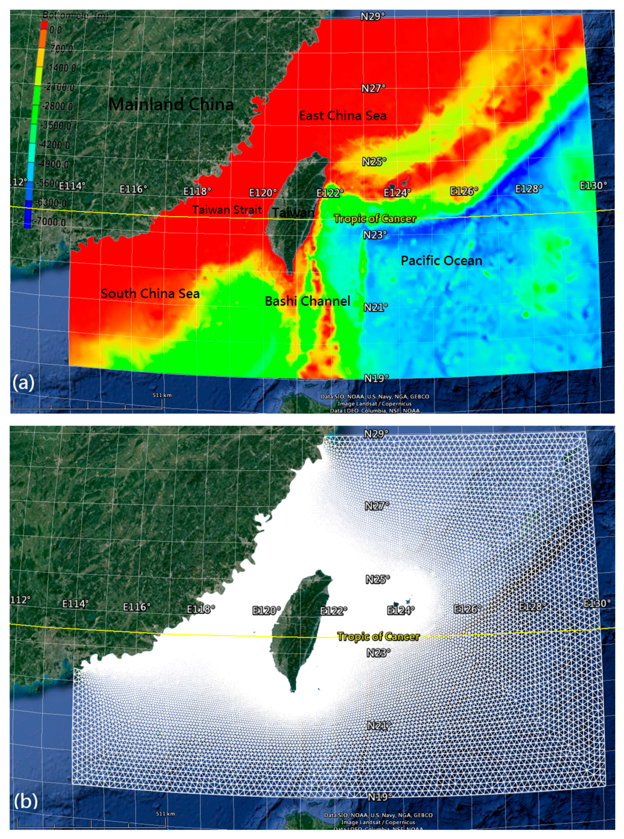
Figure 2.
Distribution of wave buoys around Taiwanese waters. The cyan area represents ocean and the white areas represent land.
Figure 2.
Distribution of wave buoys around Taiwanese waters. The cyan area represents ocean and the white areas represent land.

Figure 3.
Mode-data comparison of significant wave height (SWH) at four wave buoys. (a) Keelung; (b) Suao; (c) Hualien and (d) Penghu.
Figure 3.
Mode-data comparison of significant wave height (SWH) at four wave buoys. (a) Keelung; (b) Suao; (c) Hualien and (d) Penghu.
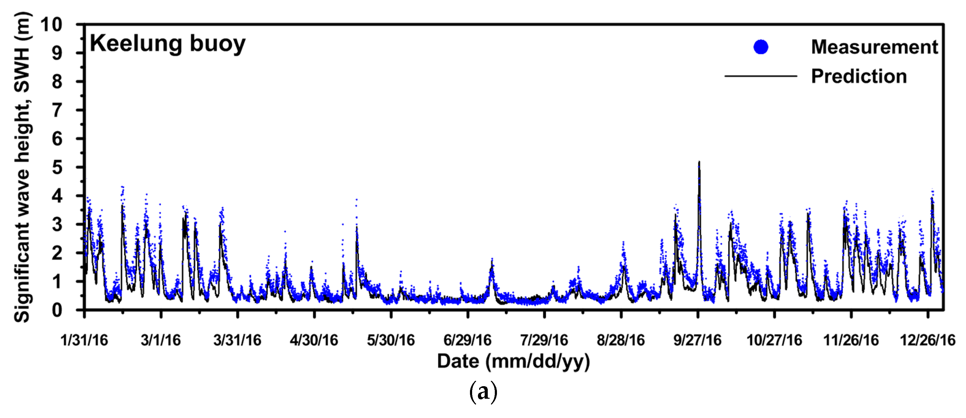
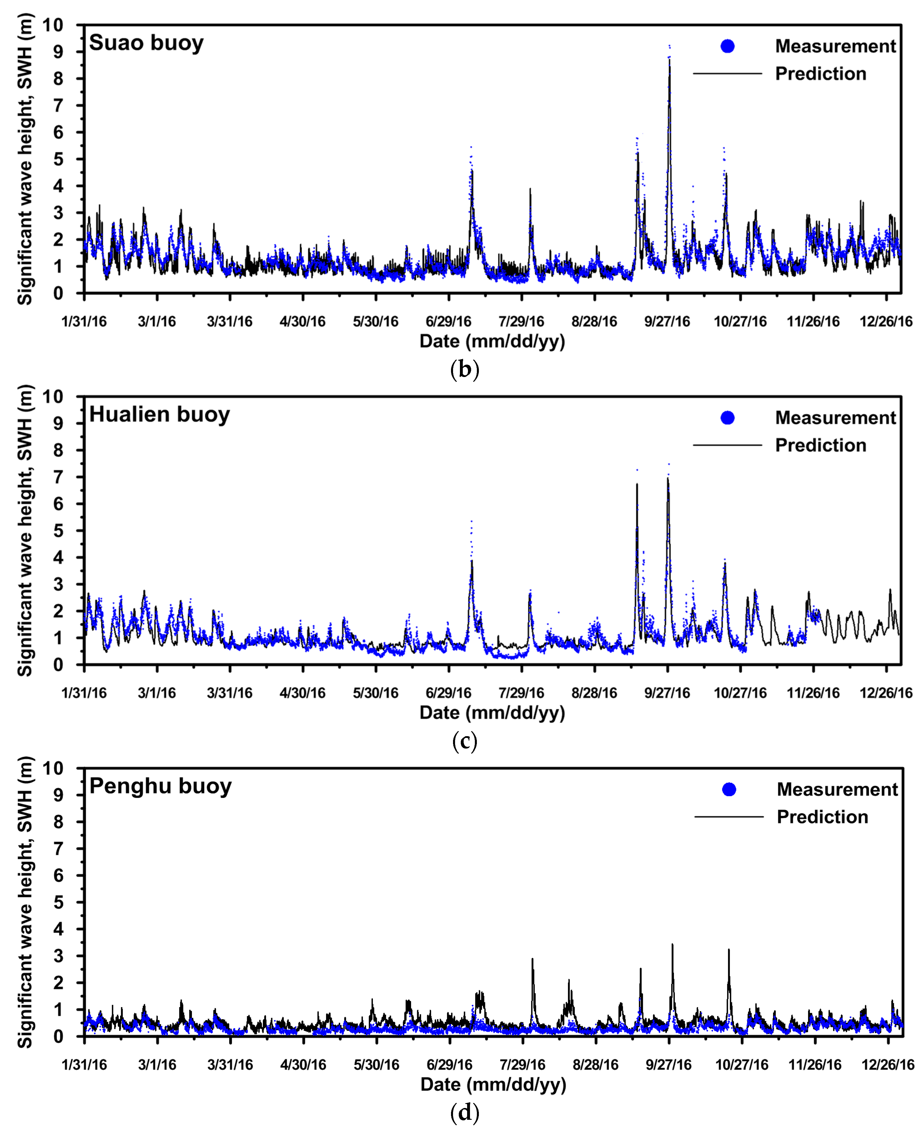
Figure 4.
Mode-data comparison of peak period (Tp) at four wave buoys. (a) Keelung; (b) Suao; (c) Hualien and (d) Penghu.
Figure 4.
Mode-data comparison of peak period (Tp) at four wave buoys. (a) Keelung; (b) Suao; (c) Hualien and (d) Penghu.
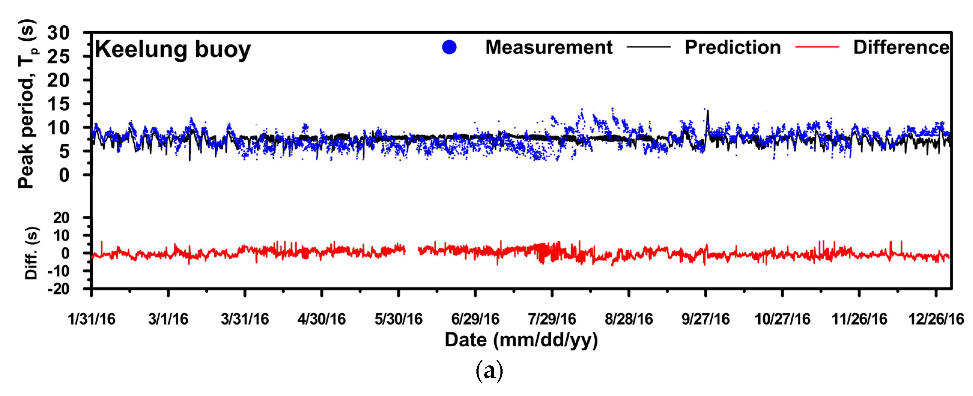
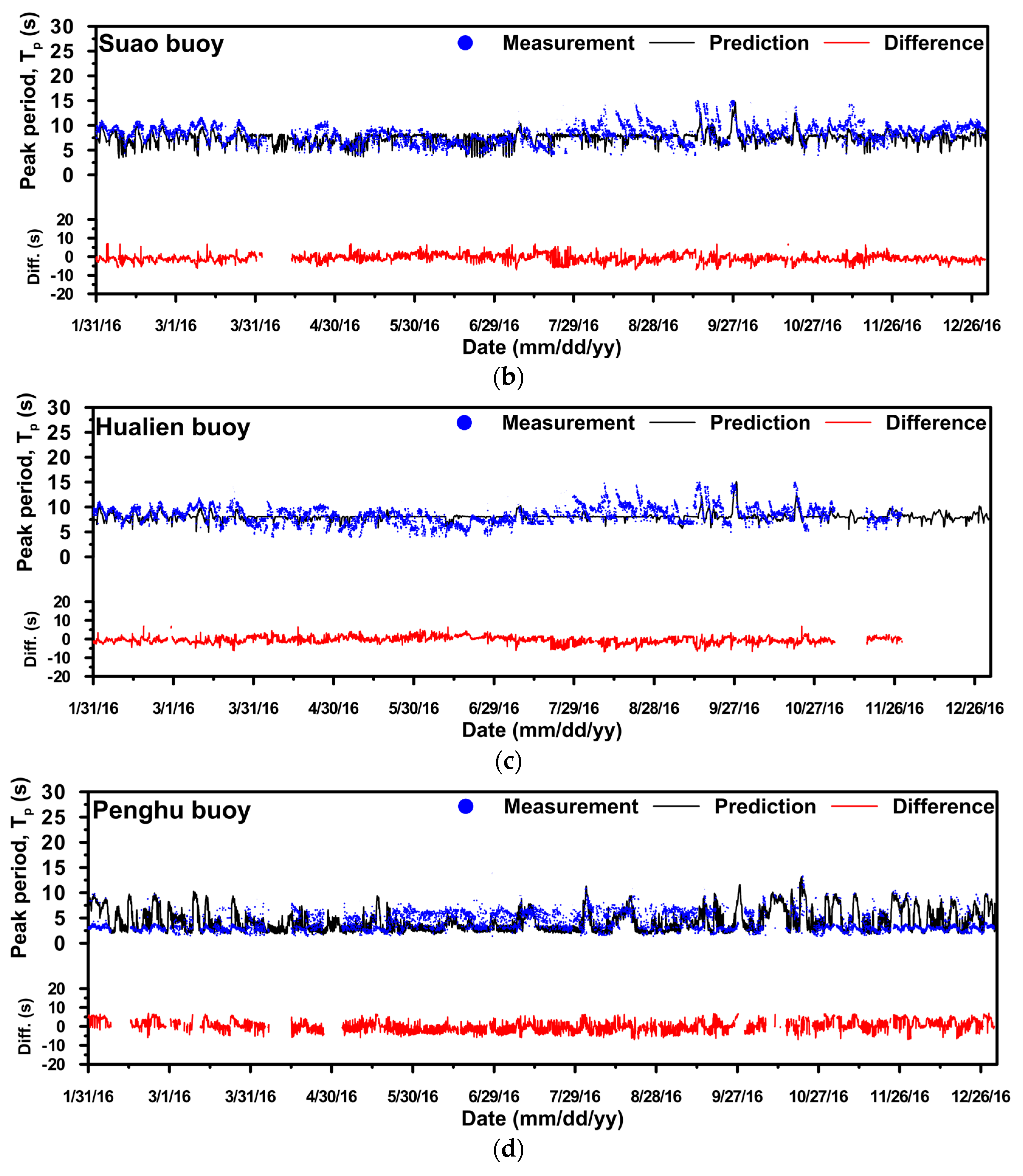
Figure 5.
Spatial distribution map of offshore annual average significant wave height (SWH) for each year from 2005 to 2016 in Taiwanese waters.
Figure 5.
Spatial distribution map of offshore annual average significant wave height (SWH) for each year from 2005 to 2016 in Taiwanese waters.

Figure 6.
Spatial distribution map of offshore 12-year (2005 to 2016) annual average significant wave height (SWH) in Taiwanese waters.
Figure 6.
Spatial distribution map of offshore 12-year (2005 to 2016) annual average significant wave height (SWH) in Taiwanese waters.
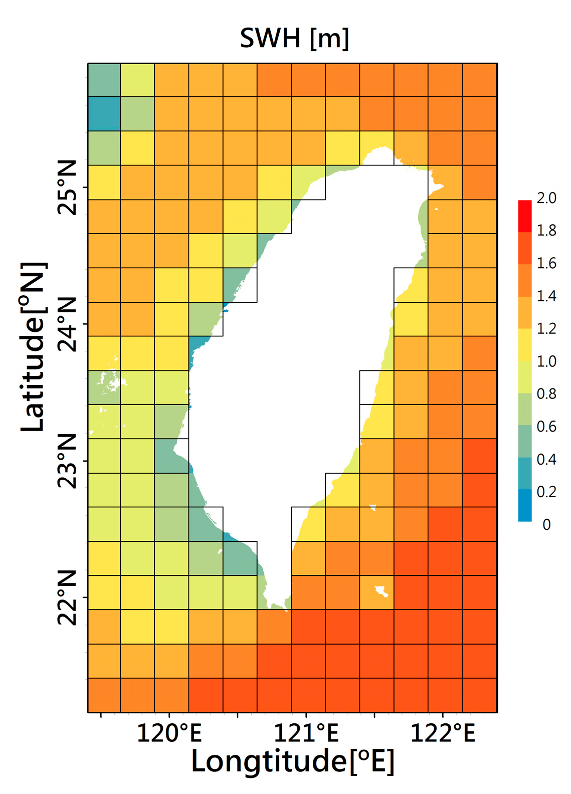
Figure 7.
Spatial distribution map of offshore annual average wave power for each year from 2005 to 2016 in Taiwanese waters.
Figure 7.
Spatial distribution map of offshore annual average wave power for each year from 2005 to 2016 in Taiwanese waters.

Figure 8.
Spatial distribution map of offshore 12-year (2005–2016) annual average wave power in Taiwanese waters.
Figure 8.
Spatial distribution map of offshore 12-year (2005–2016) annual average wave power in Taiwanese waters.

Figure 9.
Spatial distribution map of offshore 12-year annual total wave energy output with (a) a resolution of 25 × 25 km and (b) a downscaled 5 × 5 km for optimal area 1 (S1).
Figure 9.
Spatial distribution map of offshore 12-year annual total wave energy output with (a) a resolution of 25 × 25 km and (b) a downscaled 5 × 5 km for optimal area 1 (S1).

Figure 10.
Spatial distribution map of offshore 12-year annual total wave energy output with (a) a resolution of 25 × 25 km and (b) a downscaled 5 × 5 km for optimal area 2 (S2).
Figure 10.
Spatial distribution map of offshore 12-year annual total wave energy output with (a) a resolution of 25 × 25 km and (b) a downscaled 5 × 5 km for optimal area 2 (S2).

Figure 11.
Spatial distribution map of offshore 12-year annual total wave energy output with (a) a resolution of 25 × 25 km and (b) a downscaled 5 × 5 km for optimal area 3 (S3).
Figure 11.
Spatial distribution map of offshore 12-year annual total wave energy output with (a) a resolution of 25 × 25 km and (b) a downscaled 5 × 5 km for optimal area 3 (S3).
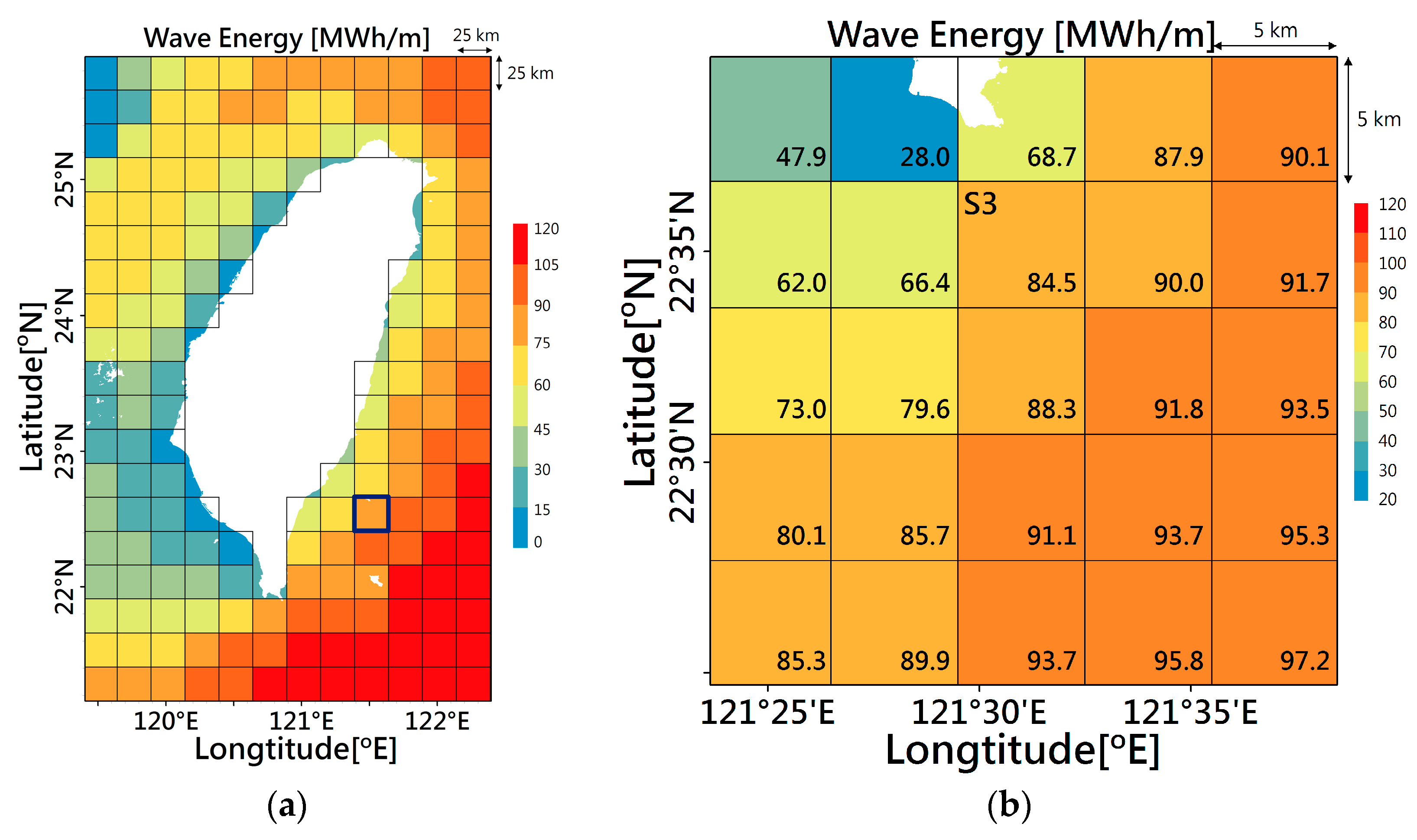
Figure 12.
Spatial distribution map of offshore 12-year annual total wave energy output with (a) a resolution of 25 × 25 km and (b) a downscaled 5 × 5 km for optimal area 4 (S4).
Figure 12.
Spatial distribution map of offshore 12-year annual total wave energy output with (a) a resolution of 25 × 25 km and (b) a downscaled 5 × 5 km for optimal area 4 (S4).

Figure 13.
Spatial distribution map of offshore 12-year annual total wave energy output with (a) a resolution of 25 × 25 km and (b) a downscaled 5 × 5 km for optimal area 5 (S5).
Figure 13.
Spatial distribution map of offshore 12-year annual total wave energy output with (a) a resolution of 25 × 25 km and (b) a downscaled 5 × 5 km for optimal area 5 (S5).
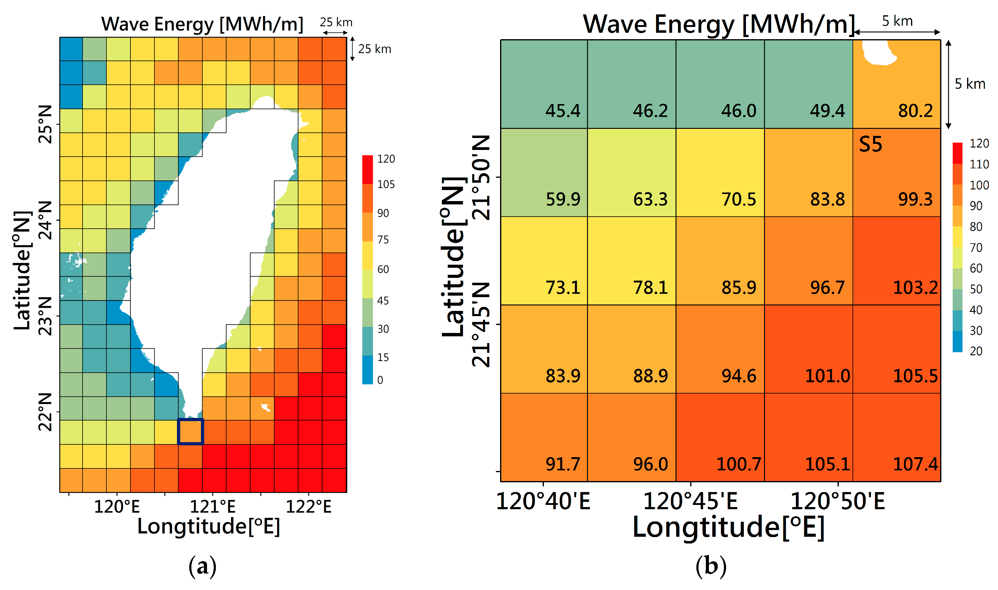
Figure 14.
Directional distributions of average wave power for five optimal areas (a) S1; (b) S2; (c) S3; (d) S4; (e) S5 for 2005–2016.
Figure 14.
Directional distributions of average wave power for five optimal areas (a) S1; (b) S2; (c) S3; (d) S4; (e) S5 for 2005–2016.


Table 1.
Central latitudes, longitudes, and average water depths of five optimal areas for wave energy converter (WEC) deployment.
Table 1.
Central latitudes, longitudes, and average water depths of five optimal areas for wave energy converter (WEC) deployment.
| Area | Longitude (°) | Latitude (°) | Depth * (m) |
|---|---|---|---|
| S1 | 121.71 | 25.23 | 100.01 |
| S2 | 122.01 | 25.03 | 123.39 |
| S3 | 121.51 | 22.58 | 1008.28 |
| S4 | 121.61 | 21.91 | 122.51 |
| S5 | 120.86 | 21.83 | 208.86 |
* Depth is below the sea level.
© 2018 by the authors. Licensee MDPI, Basel, Switzerland. This article is an open access article distributed under the terms and conditions of the Creative Commons Attribution (CC BY) license (http://creativecommons.org/licenses/by/4.0/).
Share and Cite
MDPI and ACS Style
Shih, H.-J.; Chang, C.-H.; Chen, W.-B.; Lin, L.-Y. Identifying the Optimal Offshore Areas for Wave Energy Converter Deployments in Taiwanese Waters Based on 12-Year Model Hindcasts. Energies 2018, 11, 499. https://doi.org/10.3390/en11030499
AMA Style
Shih H-J, Chang C-H, Chen W-B, Lin L-Y. Identifying the Optimal Offshore Areas for Wave Energy Converter Deployments in Taiwanese Waters Based on 12-Year Model Hindcasts. Energies. 2018; 11(3):499. https://doi.org/10.3390/en11030499
Chicago/Turabian StyleShih, Hung-Ju, Chih-Hsin Chang, Wei-Bo Chen, and Lee-Yaw Lin. 2018. "Identifying the Optimal Offshore Areas for Wave Energy Converter Deployments in Taiwanese Waters Based on 12-Year Model Hindcasts" Energies 11, no. 3: 499. https://doi.org/10.3390/en11030499
Note that from the first issue of 2016, this journal uses article numbers instead of page numbers. See further details here.