A New Hybrid Prediction Method of Ultra-Short-Term Wind Power Forecasting Based on EEMD-PE and LSSVM Optimized by the GSA


1
College of Information and Electrical Engineering, China Agricultural University, Beijing 100083, China
2
China Electric Power Research Institute, Haidian District, Beijing 100192, China
*
Author to whom correspondence should be addressed.
Energies 2018, 11(4), 697; https://doi.org/10.3390/en11040697
Submission received: 31 December 2017
/
Revised: 8 February 2018
/
Accepted: 9 February 2018
/
Published: 21 March 2018
(This article belongs to the Special Issue Hybrid Advanced Optimization Methods with Evolutionary Computation Techniques in Energy Forecasting)
Abstract
:Wind power time series data always exhibits nonlinear and non-stationary features, making it very difficult to accurately predict. In this paper, a novel hybrid wind power time series prediction model, based on ensemble empirical mode decomposition-permutation entropy (EEMD-PE), the least squares support vector machine model (LSSVM), and gravitational search algorithm (GSA), is proposed to improve accuracy of ultra-short-term wind power forecasting. To process the data, original wind power series were decomposed by EEMD-PE techniques into a number of subsequences with obvious complexity differences. Then, a new heuristic GSA algorithm was utilized to optimize the parameters of the LSSVM. The optimized model was developed for wind power forecasting and improved regression prediction accuracy. The proposed model was validated with practical wind power generation data from the Hebei province, China. A comprehensive error metric analysis was carried out to compare the performance of our method with other approaches. The results showed that the proposed model enhanced forecasting performance compared to other benchmark models.
1. Introduction
As a clean renewable energy, wind energy is regarded as a good alternative to deal with environmental problems and energy crises [1,2]. According to a report published by the World Wind Energy Association (WWEA), worldwide wind capacity reached 54 GW by the end of 2017, with a growth rate of 11.8% [3]. The total installed capacity is reported in Figure 1. The intermittent nature of wind power generation has posed a big challenge for maximizing the utilization of the wind power industry [4]. It is of practical significance to optimize the wind power prediction algorithm and make it more suitable for the operation and wind conditions of a specific wind farm.
Wind power forecasting is difficult to achieve due to its intermittency and stochastic fluctuation, which brings great challenges to power system operation and control [5,6]. Over the past few decades, a large amount of research has been devoted to the development of effective and reliable wind speed/power forecasting methods, models, and tools [7]. Generally, these methods can be broadly divided into four major models [8,9,10,11]: (a) physical models, (b) statistical models, (c) hybrid models, and (d) spatial correlation models. Physical models take into account parameters such as topography, temperature, and pressure, at the location of the wind farm, which are often utilized in short-term forecasting 6–72 h ahead and long-term forecasting with multiple weather variables. Typical physical wind power forecasting systems, among others, are the Prediktor system, developed by the Risoe National Laboratory in Denmark [12]; Previento, developed by the University of Oldenburg in Germany [13]; and eWind, developed by AWS True Wind Inc. (New York, NY, USA) [14]. Statistical models are built based on historical power/speed time series data, which establishes a functional relationship between historical data and forecast data [15]. These models analyze the relationship between various explanatory variables and online measurements. The well-known pure statistical models are the autoregressive (AR) model [16], autoregressive moving average (ARMA) model [17], autoregressive integrated moving average (ARIMA) model [18], seasonal autoregressive integrated moving average (SARIMA) model [19], and the autoregressive integrated moving average with exogenous variables (ARMAX) model [20]. However, statistical models based on the assumption that linear structures exist among time series data cannot capture non-linear patterns very well.
Individual models lack the ability to deal with big data and fail to capture the majority of the complex characteristics of the original wind power series data [21]. To make use of the advantages of statistical and physical models, a number of hybrid models with data pre-processing techniques, error post-processing techniques, and parameter selection and optimization techniques, have been proposed.
Data pre-processing techniques involve analyzing and processing data make original time series into multiple sequences or matrices, which have more obvious characteristics. Therefore, to some extent, pre-processing techniques can improve forecasting accuracy. Wavelet decomposition [22,23,24,25,26] and empirical mode decomposition [27,28,29] are the prevailing data pre-processing techniques, which can analyze the original wind power series in time and frequency domains. De et al. [25] compared the hybrid artificial neural networks (ANN) method. Case studies show that wavelet decomposition (WD)-LSSVM performs better than WD-ANN. Zhang et al. [29] used variational mode decomposition (VMD) to process original wind power series, then established a novel combined model based on machine learning methods. Zhao et al. [30] analyzed the characteristics of the outliers caused by wind curtailment, then, a data-driven outlier elimination approach, combining quartile method and density-based clustering method was proposed; however, variational mode decomposition (VMD) is prone to mode mixing problems. Niu et al. [31] used empirical mode decomposition (EMD) to decompose original wind speed data, then, a novel hybrid forecasting model based on the general regression neural network (GRNN) method, optimized by the fruit fly optimization algorithm (FOA), was proposed. Ye et al. [32] discussed EMD, EEMD, complementary ensemble empirical mode decomposition (CEEMD), and complete empirical mode decomposition with adaptive noise (CEEMDAN). Their results showed that the proposed CEEMDAN-support vector regression (CEEMDAN-SVR) model out-performed the other models.
Error post-processing (EP-P) techniques use estimated error, which is obtained from a forecasting model, to correct final forecasting results. Huang et al. [33] proposed a new, real-time decomposition model based on the feature selection and error correction of wind speed forecasting, which improved prediction accuracy. Platon et al. [34] used an advanced technique to estimate surface wind gusts, then, combined dynamic and statistical techniques into the wind power forecasting model. Liang et al. [35] improved wind speed forecasting performance using a correlation analysis method to analyze multi-step forecast errors and proposed a novel hybrid wind speed prediction model based on error forecast correction. Federica et al. [36] employed a principal component analysis (PCA), combined with post-processing, to reduce computational costs and forecast errors. Li et al. [37] proposed a new combined approach based on Extreme Learning Machine (ELM) and an error correction model, which improved prediction accuracy over a short-term time scale (6–72 h).
Parameter selection and optimization techniques can improve prediction accuracy and reduce prediction time through the training model. Xiao et al. [38] employed a new hybrid prediction model based on a modified bat algorithm (BA) with the conjugate gradient (CG) method to multi-step wind speed prediction, which optimized the initial weights of the neural networks. Wang et al. [39] proposed a novel combined forecasting model based on a multi-objective bat algorithm (MOBA), multi-step-ahead wind speed forecasting. Huang et al. [40] proposed a novel forecasting model, using a quantum particle swarm optimization (PSO) algorithm, to receive higher forecast accuracy levels. Chang et al. [41] compared the persistence method, the back propagation artificial neural network (BP) model, and radial basis neural network (RBF) model. Case studies showed that the proposed forecasting method was more accurate and reliable than the other three models. The clonal selection algorithm (CSA) [42], gravitational search algorithm (GSA) [43], particle swarm optimization (PSO) [44,45], simplified swarm optimization (SSO) [46], and cuckoo search algorithm (CS) [47], among others, are the prevailing methods to optimize the parameters of wind power/speed forecasting models.
Spatial correlation models characterize the relationship between the wind power or speed of a target wind farm and a reference wind farm at different spatial locations. Zhou et al. [48] proposed a spatial and temporal correlation model and it was found that this model could improve ultra-short-term wind power forecasting accuracy. Tascikaraoglu et al. [49] proposed a novel method, which first utilized a Wavelet Transform (WT) method to decompose the wind speed data into more stationary components and then used a spatio-temporal model on each of the subseries to incorporate both the temporal and spatial information for wind speed forecasting. Ye et al. [50] analyzed uncertainty and dependence in wind power output, and employed a physical spatio-temporal correlation model. They found that this method outperformed statistical models.
In this paper, a novel combine model is proposed based on ensemble empirical mode decomposition, permutation entropy, least squares support vector machine, and gravitational search algorithm for ultra-short wind power forecasting. To investigate the effectiveness of the model, the proposed method will be thoroughly tested and benchmarked on real wind power data from Hebei, China. The main contributions of this research will be as follows:
- (1)
- Using pre-processing techniques to deal with the complex wind power time series.
The ensemble empirical mode decomposition-permutation entropy will be used to analyze the original wind power series, by which the original wind power time series will be translated into some new, relatively stable subsequences. Ensemble empirical mode decomposition can decompose original wind power time series into a series of intrinsic mode functions (IMF) with different characteristic scales; however, it fails to capture weak changes in time series. Permutation entropy will be used to reconstitute subsequences by similar principles, which can promote weak time signals.
- (2)
- Employing the LSSVM forecasting model, optimized by GSA.
LSSVM will be employed as the basic forecasting model, due to the features of regression for wind power prediction. To improve the forecasting accuracy and stability of LSSVM directly, the hyper-parameters of LSSVM will, firstly, be optimized by GSA to obtain the best hyper-parameters.
- (3)
- Using comprehensive error metrics to assess the performance of the proposed model.
The error indicators, in this paper, will include the normalized mean absolute of errors (NMAE), normalized root mean square error (NRMSE), and Pearson correlation coefficient (R). In this paper, we will also introduce two improvement percentage error indexes, and .
The remainder of the paper will be organized as follows: the details of the proposed hybrid model based on EMD-PE-LSSVM-GSA for wind power forecasting will be illustrated in Section 2. Forecasting performance evaluation indicators will be described in Section 3. Experimental examples will be presented in Section 4. The resulting analysis and forecasting performance of the proposed method, compared with other methods, will be given in Section 5. Finally, conclusions will be given in Section 6.
2. Proposed Methodology
The approaches used, including ensemble empirical mode decomposition, permutation entropy, the least squares support vector machine model, and gravity search algorithm, are described in this section. The EEMD-PE-LSSVM-GSA wind power prediction process is shown in Figure 2.
2.1. Ensemble Empirical Mode Decomposition (EEMD)
EMD is frequently subject to a mode mixing problem, where a portion of the IMF may have properties that are quite similar to adjacent IMFs. EEMD is based on EMD and is an algorithm-based method of processing signals, which can be used to developed to solve the mode mixing problem [51]. White noise is added to the wind power time series at different scales. In order to solve the EMD mode mixing problem, a detailed explication is given in [52], as follows:
- (1)
- Add white noise series to the original wind power series:where is the original wind power series, and is the white noise series. Then, find the corresponding EMD components.
- (2)
- Find the local maxima and minima of .
- (3)
- Find the upper envelope and lower envelope .
- (4)
- Calculate the mean of the wind power time series with white noise and the difference between and .
- (5)
- Repeat Steps 1–3 with instead of , until (where is the acceptable error). Then, take as the first EMD component of , and the residual is as follows:
- (6)
- The wind power time series can be decomposed as follows:where represents the IMFs, and is the final residue.
2.2. Permutation Entropy (PE)
In the case of nonlinear analysis, the complexity of the signal can be effectively determined according to its entropy values [53], such as scale entropy, sample entropy, and multi-scale entropy. Permutation entropy is widely used in sequence complexity and nonlinear analysis because of its high robustness, efficiency, and simplicity.
This method’s motivation is the classification of the complex system. The larger the permutation entropy value, the higher the time series randomness of the sequence and the more likely another pattern will occur. Conversely, the smaller the permutation entropy value, the lower the time series randomness of the subsequence and the less likely another pattern will occur. The algorithm implementation process of PE is given below.
For time series samples, , the time series are reconstructed by m-dimension phase space.
where is the embed dimension of the wind power time series, and is the delay time.
where represents the index number of the column in which each element in the reconstruction vector resides. Each vector can be mapped to a set of symbols.
where
We calculated the probability of occurrence for each symbol sequence, , where:
In the form of Shannon entropy, the permutation entropy of the wind power time series can be expressed as:
When , reaches the maximum , the standardized processing can be achieved by:
Permutation entropy values were used to evaluate the complexity of each IMFs signal, and the adjacent entropy values were used to reconstitute IMFs into new subsequences (RS).
2.3. Least Squares Support Vector Machine (LSSVM)
The support vector machine (SVM) is an effective machine algorithm for data classification and regression [54]. SVM can overcome data over-fitting problems and improve generalization performance by minimizing structural risk instead of empirical risk. The standard SVM uses nonnegative errors in the cost function and inequality constraints, while the LSSVM uses square errors and equality constraints. Therefore, LSSVM is a variation of the standard SVM.
Considering the wind power training dataset, , is the number of training datasets, is the input vector, is the corresponding output, and is the dimension of . The optimal decision function can be constructed by mapping the input space into the high-dimension feature space as follows:
where is the nonlinear function, is the weight, and is the bias.
where is the model complexity, is the regularization parameter to balance the complex degree and approximation accuracy of the model, and is the empirical risk function. The objective function of LSSVM can be framed:
where represents the Lagrange multipliers.
Based on the Karush-Kuhn-Tucker (KKT) conditions, Equation (15) is given by:
Based on Equation (15) the following expression can be derived:
where is a dimensional vector, is the coefficient matrix, is the output matrix, , and is the kernel function on the basis of Mercer’s condition. The regression function of the LSSVM model can be described as:
The radial basis function is selected as the kernel function, which is given as follows:
where is the kernel parameter.
2.4. Gravitational Search Algorithm (GSA)
The GSA was first proposed in 2009 [55] and is a population optimization algorithm based on the law of gravity and Newton’s second law. The algorithm searches for the optimal solution by moving the particle position of the population. That is, as the algorithm iterates, the particles move continuously in the search space by the gravitation between them.
Assuming that the optimization problem can be given in (14) and (15), the particle’s position is the solution. The position of particle is defined as:
Step 1: Initialize the speed and position of random particles and calculate the fitness of each particle.
Step 2: Calculate the gravitational constant and the inertia mass of each particle:
where is the initial gravitational constant, is the decay rate, is the maximum generation, and
Step 3: Calculate the resultant particle force, which can be given as:
where is gravitation with the particles i and j, with dimension, d, at the t generation; is the passive gravitational mass related to particle i; is the small constant; and is the position of dimension, d, of particles i and j at the t generation; is the Euclidean distance between particles i and j.
Step 4: Calculate accelerated speed. According to Newton’s second law, the acceleration is obtained as follows:
Step 5: Update speed and position:
where is a random number with a uniform distribution [0,1].
Step 6: Check the termination condition. Terminate the optimization if the stopping criteria requirements are met, and, if not, repeat the procedure from step 2 to 5 until the termination condition requirements are met.
2.5. The Proposed Method for Wind Power Forecasting
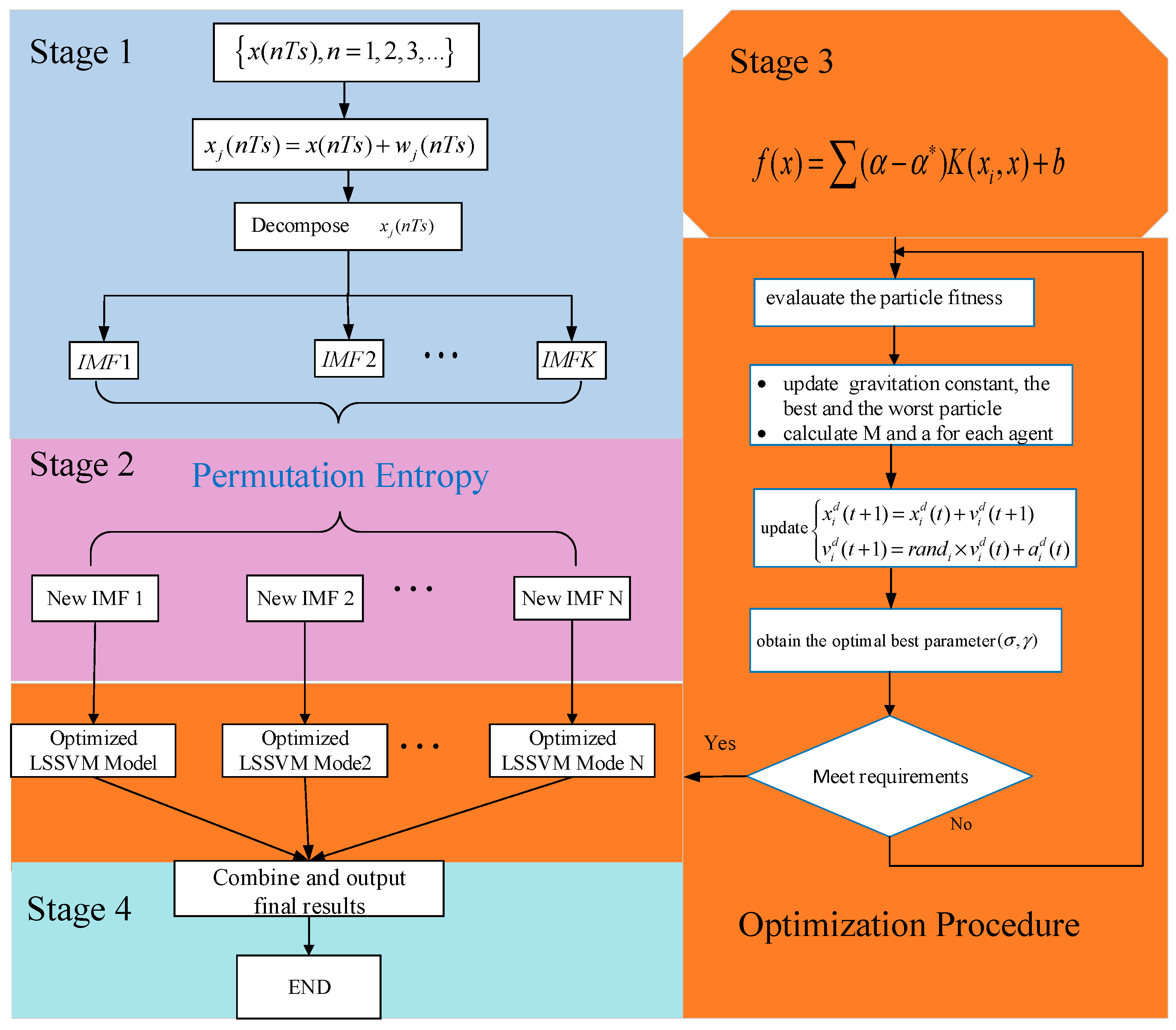
The flowchart of the proposed hybrid model based on EEMD-PE-LSSVM-GSA is illustrated in Figure 3.
Stage 1: EEMD process
To build an effective prediction model, the features of the original wind power datasets must be fully analyzed and considered. EEMD techniques can be used to decompose the original wind power time series, , into new, relatively stable subsequences,
Stage 2: PE process
PE techniques can be used to analyze the intrinsic mode signals, , and reconstitute subsequences by combination stacking, to give reconstituted subsequences, .
Stage 3: Optimize parameters in the LSSVM process
The LSSVM forecasting model can be employed to forecast the reconstituted subsequences, , and the RBF kernel functions can be chosen to initialize the LSSVM.
(1): Initialize: Setting the parameters of GSA, the particle number is L, gravitational constant is , attenuation rate is , and the dimensions of GSA are .
(2): Calculate: Calculate the fitness function as follows:
where is the real wind power value, is the forecasting value, and is the number of samples.
(3): Update: The states are updated as follows:
where is the position of the particle, is the speed of search, and is a uniform random variable, with a value in the range of [0, 1].
(4): Selection: If the iteration reaches its maximum, or the reaches its minimum, the best hyper parameters ( and ) and corresponding kernel parameters can be found.
(5): Validation: Output wind power prediction values for every new subsequence. The wind power forecasting errors, in terms of different criteria, are computed to validate the method. The results are compared with that of other methods. The best parameters of the optimized model will be obtained.
Stage 4: Hybrid process
Combine all the reconstituted subsequences of forecasting results and output the final forecasting results.
3. Performance Criterion
In this paper, the error indexes include the normalized mean absolute of errors (NMAE), which reflects actual prediction error, normalized root mean square errors (NRMSE), which reflects large forecasting deviations, and the Pearson correlation coefficient. They are defined, respectively, as follows:
where is the actual wind power value, is the forecasting value, is the installed wind power capacity, and is the number of samples.
Additionally, this paper introduces two percentage error indexes, which are defined as follows:
where a negative value of means model 2 decreases value relative to model 1, and a positive value of means model 2 increases value relative to model 1.
4. Experimental Examples
4.1. Dataset Description
In this paper, a total of 5760 samples were collected from a wind farm in Hebei, China. Considering the influence of seasonal factors, the whole dataset was divided into four parts, Datasets A, B, C, and D, which were independently used to verify the effectiveness of the proposed method. Dataset A was from 1–15 January 2016, Dataset B was from 1–15 April, Dataset C was from 1–15 July, and Dataset D was from 1–13 October. Wind power generation data were 15 min averaged values. The forecasting methods were applied over very short time horizons, of up to 4 steps (i.e., 1 h) ahead, with each step being 15 min. The samples are shown in Figure 4.
4.2. Data Processing
EEMD-PE was used to analyze the wind power series, by which the wind power time series could be translated into new, relatively stable subsequences. EEMD was also used to decompose the wind power time series into a series of IMFs with different characteristic scales. Then, PE was used to analyze the IMFs.
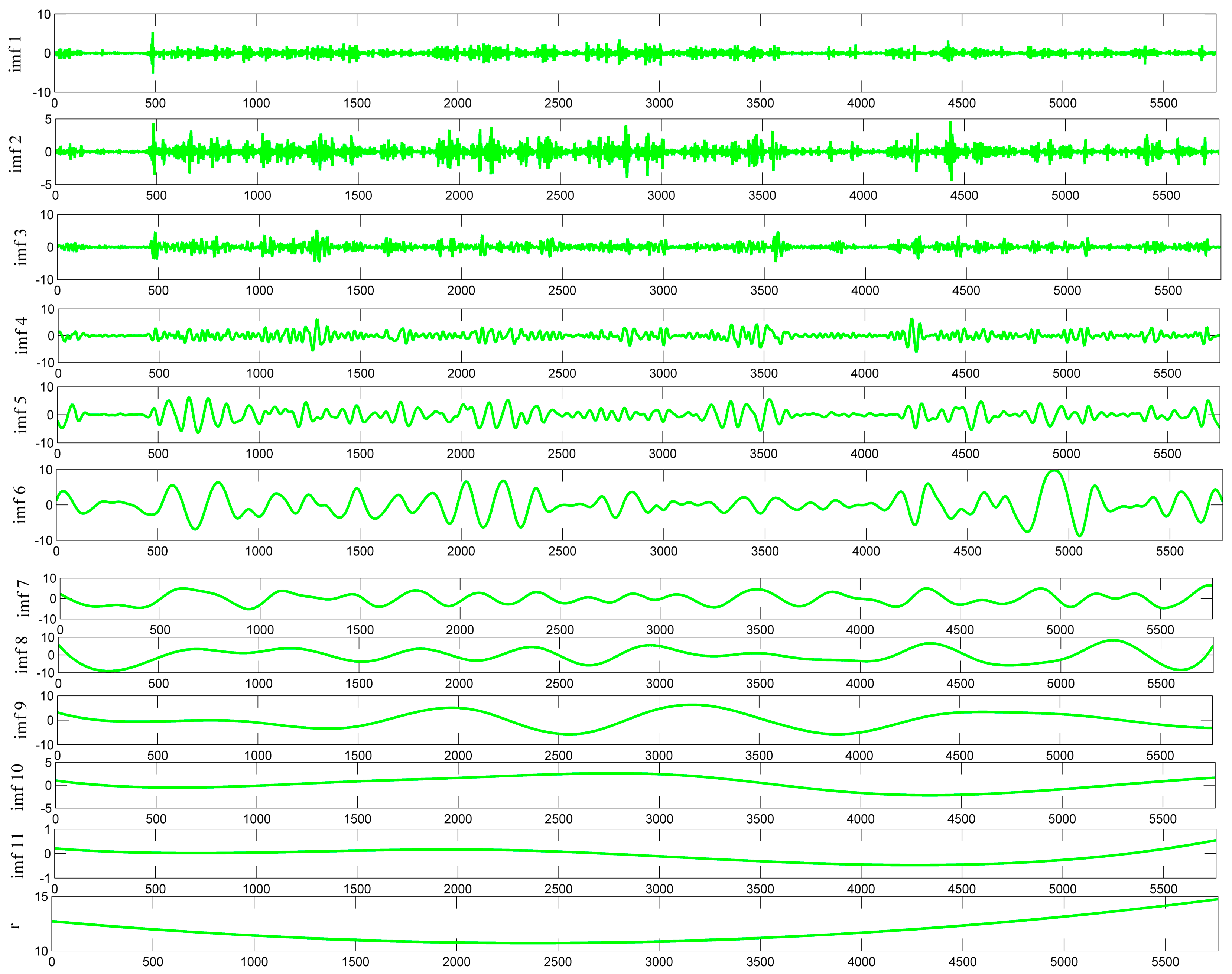
There were two important EEMD parameters: the number of the ensemble and the amplitude of the added white noise. In this experiment, 200 groups of white noise signals were added, with a standard deviation was 0.2. There were twelve independent IMF compositions. Decomposition results are shown in Figure 5.
The PE parameters ( and ) have an impact on simulation time and prediction accuracy; if the parameter is too large, prediction accuracy will be reduced, and if the parameter is too small, the simulation time will become longer. Therefore, we discuss the processing of the two parameters.
A number of different parameter values were chosen to forecast the series. It is known that the higher the embedded dimensions, the more complex the structure will be and the more modeling time will be spent. Considering the forecast time and model complexity, and models are discussed for (1–4)-step-ahead wind power forecasting, and the errors are shown in Table 1.
In Table 1, the NRMSE of and are the smallest among all parameters; then, error increases slowly with the dimension of embedding. Performance evaluation, using NMAE and NRMSE, shows that and is better than other parameters. When and , the NRMSE of the testing sample is 3.0773, which is the largest level of error, and the modeling time is 10.9929. Comparative analysis shows that increasing the embedded dimension and computation time impacts on the prediction at different time scales. Considering prediction accuracy and simulation time, and are selected to predict wind power.
Wind power time series data has nonlinear and non-stationary features. It can be seen from Figure 5 that there are a lot of IMF components after decomposition. If the LSSVM model is used to build each component respectively, the computing time will increase significantly. PE technology can be used to evaluate complexity of each IMF signal.
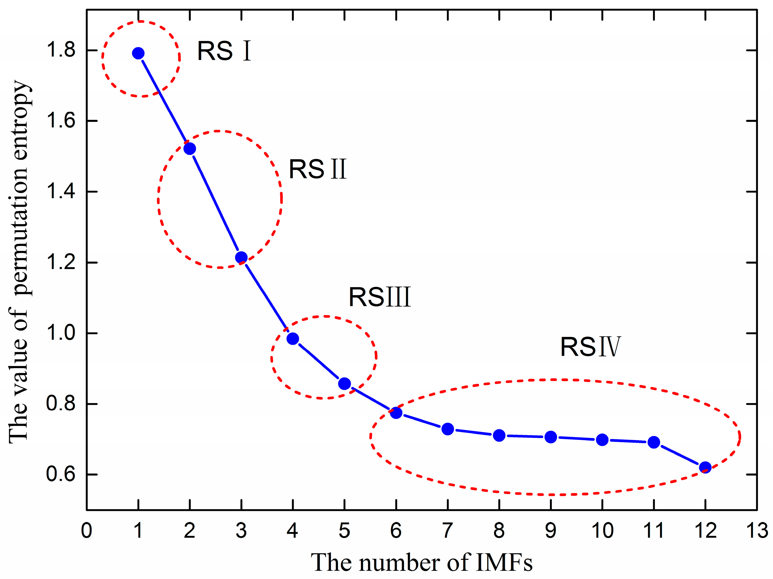
In order to forecast ultra-short-term wind power effectively, this paper used PE technology to analyze the complexity features of each IMF component. The PE values of all IMFs are shown in Figure 6. In Figure 6, the IMF component frequency decreases from high to low, and the PE value also decreases, which verifies that the PE theory is effective. The PE value indicates the stochastic degree of the time series, where a smaller PE value means more regular time series, and a larger PE value means more randomness. To reduce the computing complexity of the proposed method, according to the PE values, the IMFs were classified and merged to reconstituted subsequences. From IMF 1 to IMF 11 and residue (r), the PE values gradually decreased from 1.7916 to 0.6320. IMF 1 was assigned to RS I, since it had the highest frequency. IMF 2 and IMF 3 PE value differences were about 0.2~0.3, so they could be set as RS II. IMF 4 and IMF 5 PE value differences were about 0.1, and, thus, could be set as RS III. IMF 5~IMF 11+r PE value differences were about 0.02~0.06, and were set as RS IV. The reconstituted subsequences processed by PE are shown in Figure 7.
4.3. Parameter and Training Dataset Settings
4.3.1. The Parameter Setting of the Forecasting Models
The simulation was done on a Windows 7 PC with a 64-bit, 2.20 GHz Intel Core i3 2330M CPU, and 6 GB of memory. The wind power forecasting experiments were employed in MATLAB R2014a.
The optimal parameters, which result from using RBF kernel functions in the LSSVM model, is shown in Table 3.
4.3.2. Length of Training Datasets
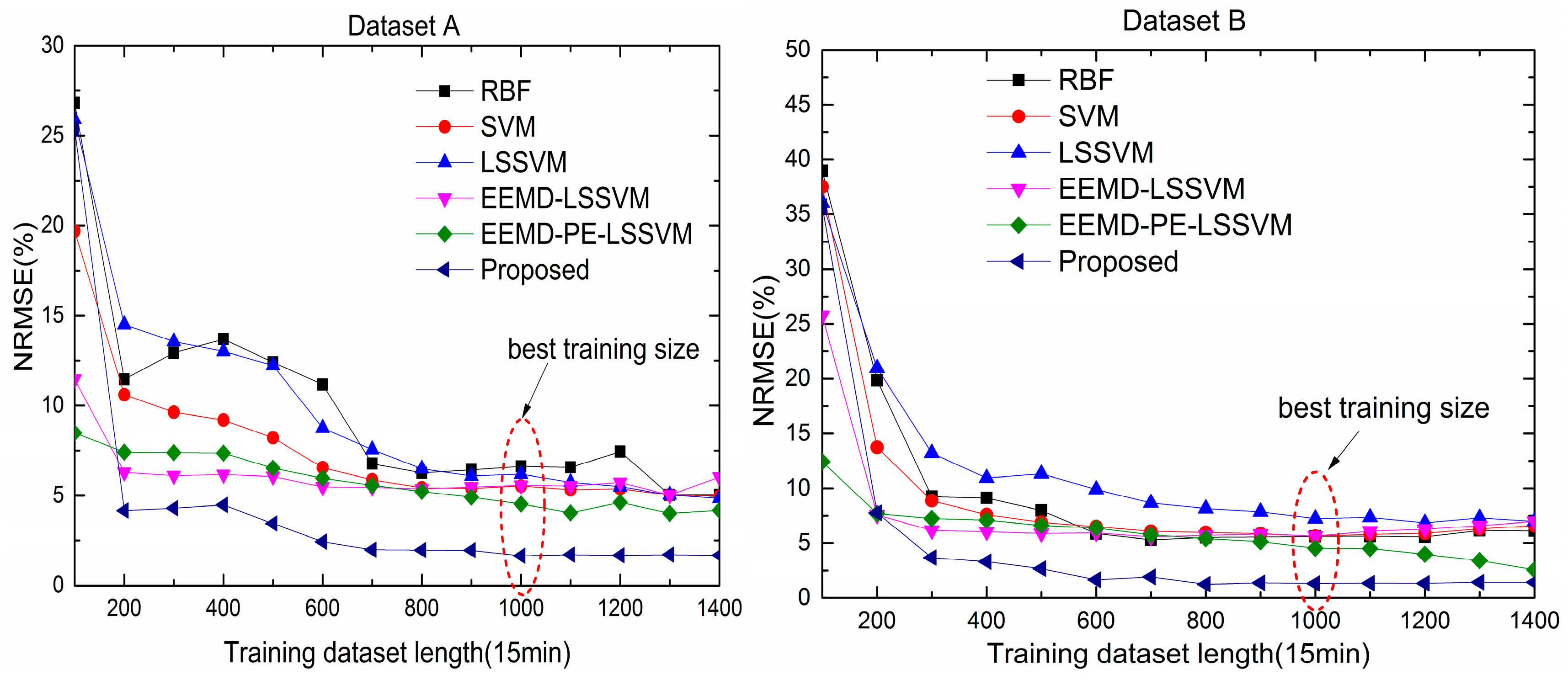
The length of training datasets is an important factor affecting prediction accuracy. The 1-step-ahead NRMSE of different forecasting methods, with training Datasets A and B, are presented in Figure 8.
In Figure 8, for Datasets A and B, the NRMSE values for six models tended to decrease with the length of the training dataset.
For Dataset A, the NRMSE of each method varied irregularly when the length of the training dataset increased from 100 to 700. The values in this interval could not be selected as the length of the training dataset. In the range of 700–1400, the trend of NRMSE became flat. The proposed model was most insensitive to training dataset length, and the NRMSE of the proposed approach remained almost unchanged as the dataset length was greater than 700, which shows the proposed model was a simple, but powerful forecasting method.
For Dataset B, the NRMSE for each method varied irregularly when the length of training dataset increased from 100 to 600. Similarly, the values in this interval could not be selected as the length of the training dataset. In the range of 600–1400, the trend of NRMSE became flat, and the other five methods remained unchanged after 1000. However, the EEMD-PE-LSSVM model kept decreasing at 1000.
Taking into account the sensitivity of each method to the data, 1000 data points, as the length of the training set, was appropriate.
5. Results and Discussion
The proposed hybrid model was employed to forecast ultra-short-term wind power, and the corresponding results from the proposed model and other contrast models are discussed in the following section.
5.1. Experiment 1: The Comparison Results of the Proposed Model and Other Models
Ultra-short-term wind power for 1-step, 2-step, 3-step and 4-step-ahead prediction was implemented for Datasets A, B, C, and D. Results from the analyses will be clearly demonstrated in Table 4, Table 5, Table 6 and Table 7 to reveal the effectiveness of each model.
To further verify the applicability, performance, and superiority of the proposed hybrid model, the wind power data from Datasets A, B, C, and D were employed for modeling, with five alternative forecasting models (the SVM model, RBF model, LSSVM model, EEMD-LSSVM model, and EEMD-PE-LSSVM model) that were compared with the proposed hybrid model. The results are shown in Figure 9, Figure 10, Figure 11 and Figure 12 and Table 4, Table 5, Table 6 and Table 7.
In Figure 9, Figure 10, Figure 11 and Figure 12, it can be seen that the error of prediction results for the proposed model was much smaller than the SVM model, RBF model, LSSVM model, EEMD-LSSVM model, and EEMD-PE-LSSVM, which implies that the proposed method performs much better than other five models. The prediction results of the EEMD-PE-LSSVM model lagged behind the proposed model for all forecasting time horizons. The forecasting results of the RBF model were the worst compared to the other models.
In order to test the accuracy of wind power forecasting, NRMSE, NMAE, R, , and were used in this paper, for Datasets A, B, C, and D with 1-step-ahead and 4-steps-ahead. Detailed numerical analysis is given in Table 4, Table 5, Table 6 and Table 7.
It can be observed from Table 4, Table 5, Table 6 and Table 7 that the NRMSE and NMAE values of the proposed method were the lowest and the R values were the highest, compared with other models for (1–4)-step-ahead prediction during the entire evaluation period, which demonstrates the superior performance of the proposed method. For all the forecasting horizons investigated in this paper, the proposed method always reached the minimum values of NRMSE and NMAE and the maximum value of R. This indicates that the proposed model significantly outperforms benchmark models. Thus, the proposed model is an effective tool for wind power forecasting.
5.2. Experiment II: Comparison Results of Improvement Percentage Error Indexes and Modeling Time
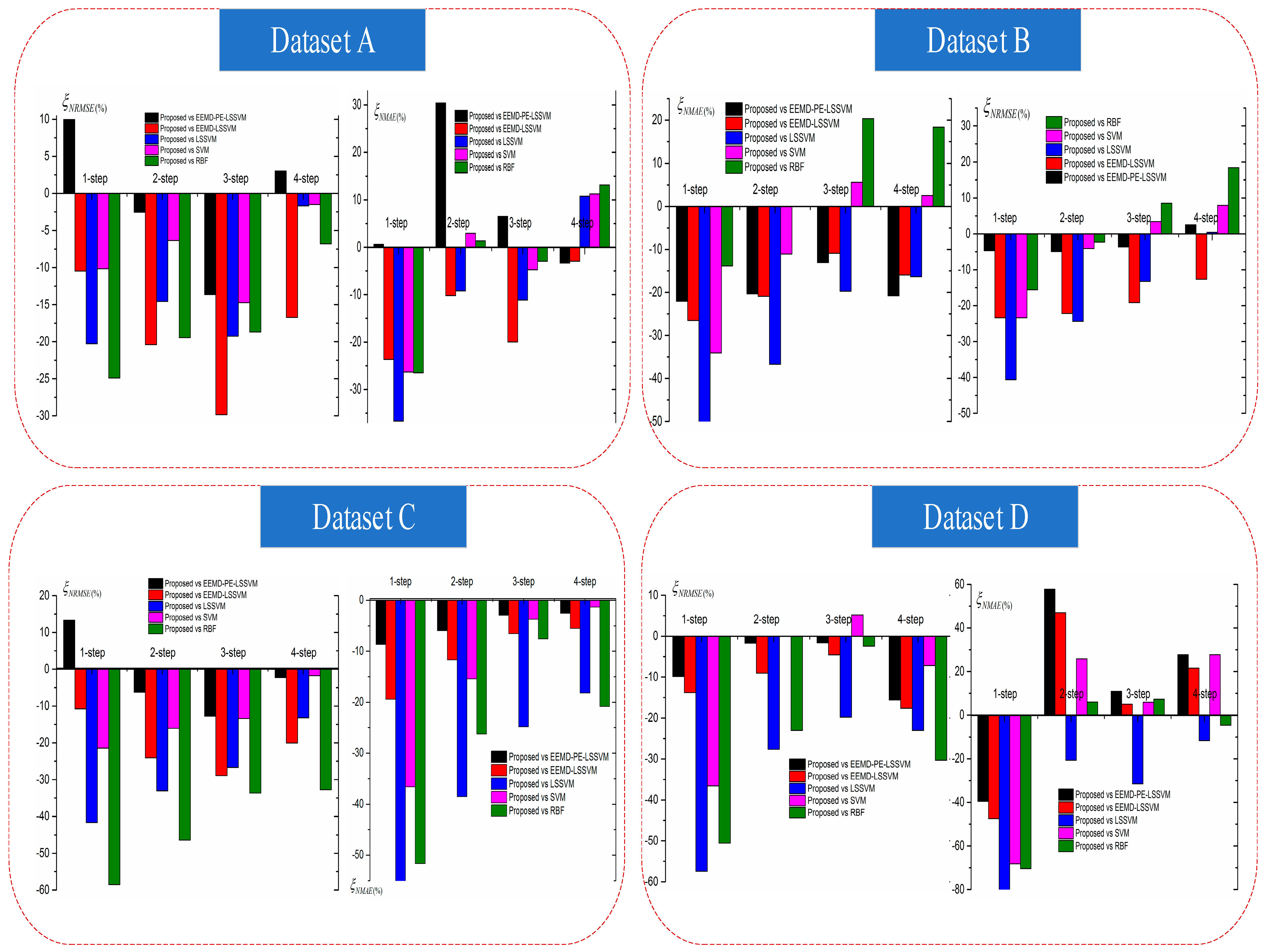
In order to compare performance differences between the combined model and other benchmark models, and were utilized in this study. By using this type of criterion, the improvement percentage values of the proposed model and benchmark models are given in Figure 13.
The histogram of and for all models regarding Datasets A, B, C, and D for (1–4)-step-ahead wind power forecasting are shown in Figure 13. For Dataset A, except for the 1- and 4-step-ahead forecasting, the values of the proposed method compared with EEMD-PE-LSSVM were positive, which shows that the performance of the proposed model was worse than the EEMD-PE-LSSVM model. In the 1-step-ahead forecasting, the negative value of for the proposed method, compared with the RBF model, was minimal, which indicates that the forecasting performance of the proposed model was powerful. In the 2-, 3- and 4-step-ahead forecasting, the proposed method, compared with the EEMD-LSSVM model, performed best.
In (1–3)-step-ahead forecasting, the proposed method had a positive value of compared with EEMD-PE-LSSVM, which shows that the proposed model was worse than the EEMD-PE-LSSVM model. In the 4-step ahead forecasting, the proposed model was slightly worse than the RBF, SVM, and LSSVM models.
There were similar results for Datasets B, C, and D, which shows that the proposed model was effective for ultra-short-term wind power prediction.
As demonstrated in Figure 13, we can derive the following conclusions: (a) heuristic algorithms have good optimization capabilities in wind power forecasting; (b) hybrid models obtain better performance compared with individual and other combined models without optimization; and (c) the proposed model performed the best among all of the studied models.
The simulation time of the 4-step-ahead wind power forecasting, with regard to Datasets A, B, C, and D, for all methods, is given in Table 8. Although the simulation time of the proposed method had higher time consumption than the other prediction models, it achieved the best prediction accuracy, and this simulation time is acceptable in practical implementation.
6. Conclusions
A new hybrid prediction method of ultra-short-term wind power forecasting, based on EEMD-PE and LSSVM optimization by GSA, was proposed in this paper. The EEMD method was used to decompose raw wind power data time series into a series of IMFs with different scales to solve the mode mixing problem. To effectively reduce the computational complexity of the combined forecasting method, PE was introduced into the complexity assessment of each IMF component, based on the PE value, then the IMF components were recombined to generate new subsequences with significant differences in complexity. The GSA model was utilized to optimize the parameters of LSSVM, which avoided the choice of parameters; then, the optimized model was used in wind power forecasting, which improved regression prediction accuracy. For a fair, clear, comparative study, the proposed method was tested on a practical wind farm (in Hebei, China) and compared with several other models, including the EEMD-PE-LSSVM, EEMD-LSSVM, LSSVM, SVM, and RBF models. The results of the experiments indicated that the proposed model satisfactorily forecasted ultra-short-term wind power for the different datasets.
Acknowledgments
This work was supported by the National Natural Science Foundation of China (Project No. 51477174, 51677188, and 51711530227), National Key Research and Development Program of China (Project No. 2017YFB0902200), Project of State Grids Corporation of China (Project No. 5201011600TS), and the Open Fund of State Key Laboratory of Operation and Control of Renewable Energy and Storage Systems (Project No. TSTE-00833-2016).
Author Contributions
Peng Lu designed the research and wrote the paper; Lin Ye provided professional guidance; Bohao Sun, Jingzhu Teng, Cihang Zhang, and Yongning Zhao translated and revised this paper.
Conflicts of Interest
The authors declare no conflict of interest.
Abbreviations
| the original wind power series | NRMSE | the normalized root mean square error | |
| the white noise series | NMAE | the normalized mean absolute error | |
| the wind power series with white noise | pearson correlation coefficient | ||
| N | the total number of data | EMD | empirical mode decomposition |
| a set of symbols | EEMD | ensemble empirical mode decomposition | |
| the probability of each symbol sequence | VMD | variational mode decomposition | |
| the permutation entropy | WT | wavelet Transform | |
| RS | reconstitute subsequences | WD | wavelet decomposition |
| is the nonlinear function | SVM | support vector machine | |
| the weight | LSSVM | least squares support vector machine | |
| the bias | RBF | radial basis neural network | |
| the empirical risk function | GA | genetic algorithm | |
| the gravitational constant | SSO | simplified swarm optimization | |
| the initial gravitational constant | CSA | clonal selection algorithm | |
| the decay rate | PSO | particle swarm optimization | |
| the maximum generation | FFA | firefly optimization algorithm | |
| acceleration | GSA | gravitational search algorithm | |
| the speed of particle ith in dimension | MOBA | multi-objective bat algorithm | |
| the position of particle ith in dimension | BP | back propagation artificial neural network | |
| the actual wind power value | BA | bat algorithm | |
| the forecasting value |
References
- Zhao, Y.; Ye, L.; Li, Z.; Song, X.; Lang, Y.; Su, J. A novel bidirectional mechanism based on time series model for wind power forecasting. Appl. Energy 2016, 177, 793–803. [Google Scholar] [CrossRef]
- Lydia, M.; Kumar, S.S.; Selvakumar, A.I.; Kumar, G.E.P. A comprehensive review on wind turbine power curve modeling techniques. Renew. Sust. Energy Rev. 2014, 30, 452–460. [Google Scholar] [CrossRef]
- World Wind Market Has Reached 486 GW from Where 54 GW Has Been Installed Last Year. Available online: http://www.wwindea.org/11961-2/ (accessed on 23 January 2018).
- Ren, G.; Liu, J.; Wan, J.; Guo, Y.; Yu, D.; Yan, J. Overview of wind power intermittency: Impacts, measurements, and mitigation solutions. Appl. Energy 2017, 204, 47–65. [Google Scholar] [CrossRef]
- Liu, Y.Q.; Sun, Y.; Infield, D.; Zhao, Y.; Han, S.; Yan, J. A hybrid forecasting method for wind power ramp based on orthogonal test and support vector machine (ot-svm). IEEE Trans. Sustain. Energy 2017, 8, 451–457. [Google Scholar] [CrossRef]
- Jiang, Y.; Chen, X.Y.; Yu, K.; Liao, Y.C. Short-term wind power forecasting using hybrid method based on enhanced boosting algorithm. J. Mod. Power Syst. Clean Energy 2017, 5, 126–133. [Google Scholar] [CrossRef]
- Alencar, D.B.D.; Affonso, C.D.M.; Oliveira, R.L.D.; Rodríguez, J.M.; Leite, J.; Filho, J.R. Different models for forecasting wind power generation: Case study. Energies 2017, 10, 1976. [Google Scholar]
- Tascikaraoglu, A.; Uzunoglu, M. A review of combined approaches for prediction of short-term wind speed and power. Renew. Sust. Energy Rev. 2014, 34, 243–254. [Google Scholar] [CrossRef]
- Dong, L.; Wang, L.J.; Khahro, S.F.; Gao, S.; Liao, X.Z. Wind power day-ahead prediction with cluster analysis of nwp. Renew. Sust. Energy Rev. 2016, 60, 1206–1212. [Google Scholar] [CrossRef]
- Chang, W.Y. A literature review of wind forecasting methods. J. Power Energy Eng. 2014, 2, 161–168. [Google Scholar] [CrossRef]
- Genikomsakis, K.N.; Lopez, S.; Dallas, P.I.; Ioakimidis, C.S. Simulation of wind-battery microgrid based on short-term wind power forecasting. Appl. Sci. 2017, 7, 1142. [Google Scholar] [CrossRef]
- Landberg, L.; Watson, S.J. Short-term prediction of local wind conditions. Bound.-Layer Meteorol. 1994, 70, 171–195. [Google Scholar] [CrossRef]
- Focken, U.; Lange, M.; Waldl, H.-P. Previento-a wind power prediction system with an innovative upscaling algorithm. In Proceedings of the European Wind Energy Conference, Copenhagen, Denmark, 2–6 July 2001. [Google Scholar]
- Development and Testing of Improved Statistical Wind Power Forecasting Methods. Available online: digital.library.unt.edu/ark:/67531/metadc829494/ (accessed on 23 January 2018).
- Aggarwal, S.K. Wind power forecasting: A review of statistical models. Int. J. Energy Sci. 2013, 3, 1–10. [Google Scholar]
- Lydia, M.; Kumar, S.S.; Selvakumar, A.I.; Kumar, G.E.P. Linear and non-linear autoregressive models for short-term wind speed forecasting. Energy Convers. Manag. 2016, 112, 115–124. [Google Scholar] [CrossRef]
- Jiang, W.; Yan, Z.; Feng, D.H.; Hu, Z. Wind speed forecasting using autoregressive moving average/generalized autoregressive conditional heteroscedasticity model. Eur. Trans. Electr. Power 2012, 22, 662–673. [Google Scholar] [CrossRef]
- Abdelaziz, A.Y.; Rahman, M.A.; El-Khayat, M.M.; Hakim, M.A. Short term wind power forecasting using autoregressive integrated moving average approach. J. Energy Power Eng. 2013, 7, 2089. [Google Scholar]
- Fang, T.; Lahdelma, R. Evaluation of a multiple linear regression model and sarima model in forecasting heat demand for district heating system. Appl. Energy 2016, 179, 544–552. [Google Scholar] [CrossRef]
- Maggina, A. Market-Based Accounting Research (Mbar) Models: A Test of Arimax Modeling; Springer: New York, NY, USA, 2015; pp. 279–298. [Google Scholar]
- Costa, A.; Crespo, A.; Navarro, J.; Lizcano, G.; Madsen, H.; Feitosa, E. A review on the young history of the wind power short-term prediction. Renew. Sust. Energy Rev. 2008, 12, 1725–1744. [Google Scholar] [CrossRef] [Green Version]
- Kiplangat, D.C.; Asokan, K.; Kumar, K.S. Improved week-ahead predictions of wind speed using simple linear models with wavelet decomposition. Renew. Energy 2016, 93, 38–44. [Google Scholar] [CrossRef]
- Liu, H.; Tian, H.Q.; Li, Y.F. Comparison of new hybrid feemd-mlp, feemd-anfis, wavelet packet-mlp and wavelet packet-anfis for wind speed predictions. Energy Convers. Manag. 2015, 89, 1–11. [Google Scholar] [CrossRef]
- Liu, D.; Niu, D.; Wang, H.; Fan, L. Short-term wind speed forecasting using wavelet transform and support vector machines optimized by genetic algorithm. Renew. Energy 2014, 62, 592–597. [Google Scholar] [CrossRef]
- Giorgi, M.G.D.; Campilongo, S.; Ficarella, A.; Congedo, P.M. Comparison between wind power prediction models based on wavelet decomposition with least-squares support vector machine (LS-SVM) and artificial neural network (ANN). Energies 2014, 7, 5251–5272. [Google Scholar] [CrossRef]
- Jyothi, M.N.; Rao, P.R. Very-short term wind power forecasting through adaptive wavelet neural network. In Proceedings of the 2016 Biennial International Conference on Power and Energy Systems: Towards Sustainable Energy (PESTSE), Bangalore, India, 21–23 January 2016; pp. 1–6. [Google Scholar]
- Guo, Z.; Zhao, W.; Lu, H.; Wang, J. Multi-step forecasting for wind speed using a modified emd-based artificial neural network model. Renew. Energy 2012, 37, 241–249. [Google Scholar] [CrossRef]
- Fan, G.F.; Peng, L.L.; Zhao, X.; Hong, W.C. Applications of hybrid emd with pso and ga for an svr-based load forecasting model. Energies 2017, 10, 1713. [Google Scholar] [CrossRef]
- Zhang, Y.; Liu, K.; Qin, L.; An, X. Deterministic and probabilistic interval prediction for short-term wind power generation based on variational mode decomposition and machine learning methods. Energy Convers. Manag. 2016, 112, 208–219. [Google Scholar] [CrossRef]
- Zhao, Y.; Ye, L.; Wang, W.; Sun, H.; Ju, Y.; Tang, Y. Data-driven correction approach to refine power curve of wind farm under wind curtailment. IEEE Trans. Sustain. Energy 2018, 9, 95–105. [Google Scholar] [CrossRef]
- Niu, D.; Liang, Y.; Hong, W.-C. Wind speed forecasting based on emd and grnn optimized by foa. Energies 2017, 10, 2001. [Google Scholar] [CrossRef]
- Ren, Y.; Suganthan, P.N.; Srikanth, N. A comparative study of empirical mode decomposition-based short-term wind speed forecasting methods. IEEE Trans. Sustain. Energy 2014, 6, 236–244. [Google Scholar] [CrossRef]
- Jiang, Y.; Huang, G. Short-term wind speed prediction: Hybrid of ensemble empirical mode decomposition, feature selection and error correction. Energy Convers. Manag. 2017, 144, 340–350. [Google Scholar] [CrossRef]
- Patlakas, P.; Drakaki, E.; Galanis, G.; Spyrou, C.; Kallos, G. Wind Gust Estimation by Combining a Numerical Weather Prediction Model and Statistical Post-Processing; EGU: Munich, Germany, 2017. [Google Scholar]
- Liang, Z.; Liang, J.; Wang, C.; Dong, X.; Miao, X. Short-term wind power combined forecasting based on error forecast correction. Energy Convers. Manag. 2016, 119, 215–226. [Google Scholar] [CrossRef]
- Davò, F.; Alessandrini, S.; Sperati, S.; Monache, L.D.; Airoldi, D.; Vespucci, M.T. Post-processing techniques and principal component analysis for regional wind power and solar irradiance forecasting. Sol. Energy 2016, 134, 327–338. [Google Scholar] [CrossRef]
- Li, Z.; Ye, L.; Zhao, Y.; Song, X.; Teng, J.; Jin, J. Short-term wind power prediction based on extreme learning machine with error correction. Prot. Control Mod. Power Syst. 2016, 1. [Google Scholar] [CrossRef]
- Xiao, L.; Qian, F.; Shao, W. Multi-step wind speed forecasting based on a hybrid forecasting architecture and an improved bat algorithm. Energy Convers. Manag. 2017, 143, 410–430. [Google Scholar] [CrossRef]
- Wang, J.; Heng, J.; Xiao, L.; Wang, C. Research and application of a combined model based on multi-objective optimization for multi-step ahead wind speed forecasting. Energy 2017, 125, 591–613. [Google Scholar] [CrossRef]
- Huang, M.L. Hybridization of chaotic quantum particle swarm optimization with svr in electric demand forecasting. Energies 2016, 9, 426. [Google Scholar] [CrossRef]
- Chang, W.Y. Short-term wind power forecasting using the enhanced particle swarm optimization based hybrid method. Energies 2013, 6, 4879–4896. [Google Scholar] [CrossRef]
- Chitsaz, H.; Amjady, N.; Zareipour, H. Wind power forecast using wavelet neural network trained by improved clonal selection algorithm. Energy Convers. Manag. 2015, 89, 588–598. [Google Scholar] [CrossRef]
- Yuan, X.; Chen, C.; Yuan, Y.; Huang, Y.; Tan, Q. Short-term wind power prediction based on LSSVM–GSA model. Energy Convers. Manag. 2015, 101, 393–401. [Google Scholar] [CrossRef]
- Osório, G.J.; Matias, J.C.O.; Catalão, J.P.S. Short-term wind power forecasting using adaptive neuro-fuzzy inference system combined with evolutionary particle swarm optimization, wavelet transform and mutual information. Renew. Energy 2015, 75, 301–307. [Google Scholar] [CrossRef]
- Dong, Z.; Yang, D.; Reindl, T.; Walsh, W.M. A novel hybrid approach based on self-organizing maps, support vector regression and particle swarm optimization to forecast solar irradiance. Energy 2015, 82, 570–577. [Google Scholar] [CrossRef]
- Yeh, W.C.; Yeh, Y.M.; Chang, P.C.; Ke, Y.C.; Chung, V. Forecasting wind power in the mai liao wind farm based on the multi-layer perceptron artificial neural network model with improved simplified swarm optimization. Int. J. Electr. Power Energy Syst. 2014, 55, 741–748. [Google Scholar] [CrossRef]
- Xiao, L.; Shao, W.; Yu, M.; Ma, J.; Jin, C. Research and application of a hybrid wavelet neural network model with the improved cuckoo search algorithm for electrical power system forecasting. Appl. Energy 2017, 198, 203–222. [Google Scholar] [CrossRef]
- Zhou, H.; Xue, Y.; Guo, J.; Chen, J. Ultra-short-term wind speed forecasting method based on spatial and temporal correlation models. J. Eng. 2017, 2017, 1071–1075. [Google Scholar]
- Tascikaraoglu, A.; Sanandaji, B.M.; Poolla, K.; Varaiya, P. Exploiting sparsity of interconnections in spatio-temporal wind speed forecasting using wavelet transform. Appl. Energy 2016, 165, 735–747. [Google Scholar] [CrossRef]
- Ye, L.; Zhao, Y.; Zeng, C.; Zhang, C. Short-term wind power prediction based on spatial model. Renew. Energy 2017, 101, 1067–1074. [Google Scholar] [CrossRef]
- Huang, N.E.; Shen, Z.; Long, S.R.; Wu, M.C.; Shih, H.H.; Zheng, Q.; Yen, N.C.; Chi, C.T.; Liu, H.H. The empirical mode decomposition and the hilbert spectrum for nonlinear and non-stationary time series analysis. Proc. Math. Phys. Eng. Sci. 1998, 454, 903–995. [Google Scholar] [CrossRef]
- Wu, Z.; Huang, N.E. Ensemble empirical mode decomposition: A noise-assisted data analysis method. Adv. Adapt. Data Anal. 2009, 1, 1–41. [Google Scholar] [CrossRef]
- Bandt, C.; Pompe, B. Permutation entropy: A natural complexity measure for time series. Phys. Rev. Lett. 2002, 88, 174102. [Google Scholar] [CrossRef] [PubMed]
- Wu, Q.; Peng, C. Wind power grid connected capacity prediction using lssvm optimized by the bat algorithm. Energies 2015, 8, 14346–14360. [Google Scholar] [CrossRef]
- Xing, B.; Gao, W.J. Gravitational Search Algorithm; Springer International Publishing: Berlin, Germanuy, 2014; pp. 355–364. [Google Scholar]
Figure 1.
Total installed wind power from 2005 to 2017 worldwide.
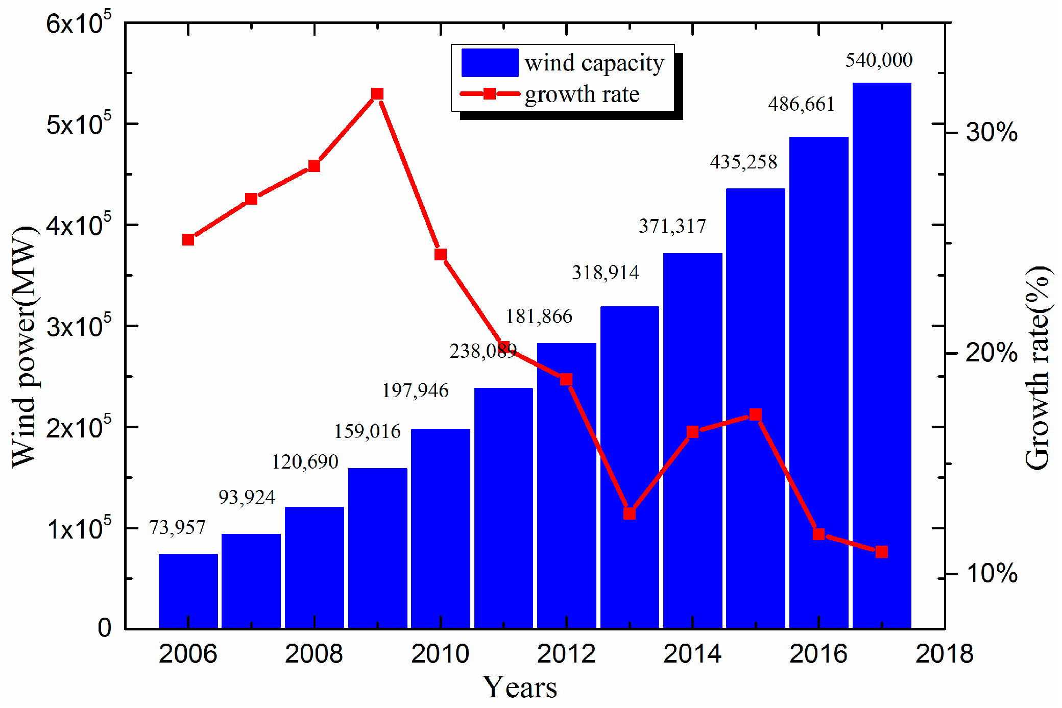
Figure 2.
The procedure of the new proposed prediction model.

Figure 3.
The overall framework of the proposed model.

Figure 4.
Time samples from Hebei, China.
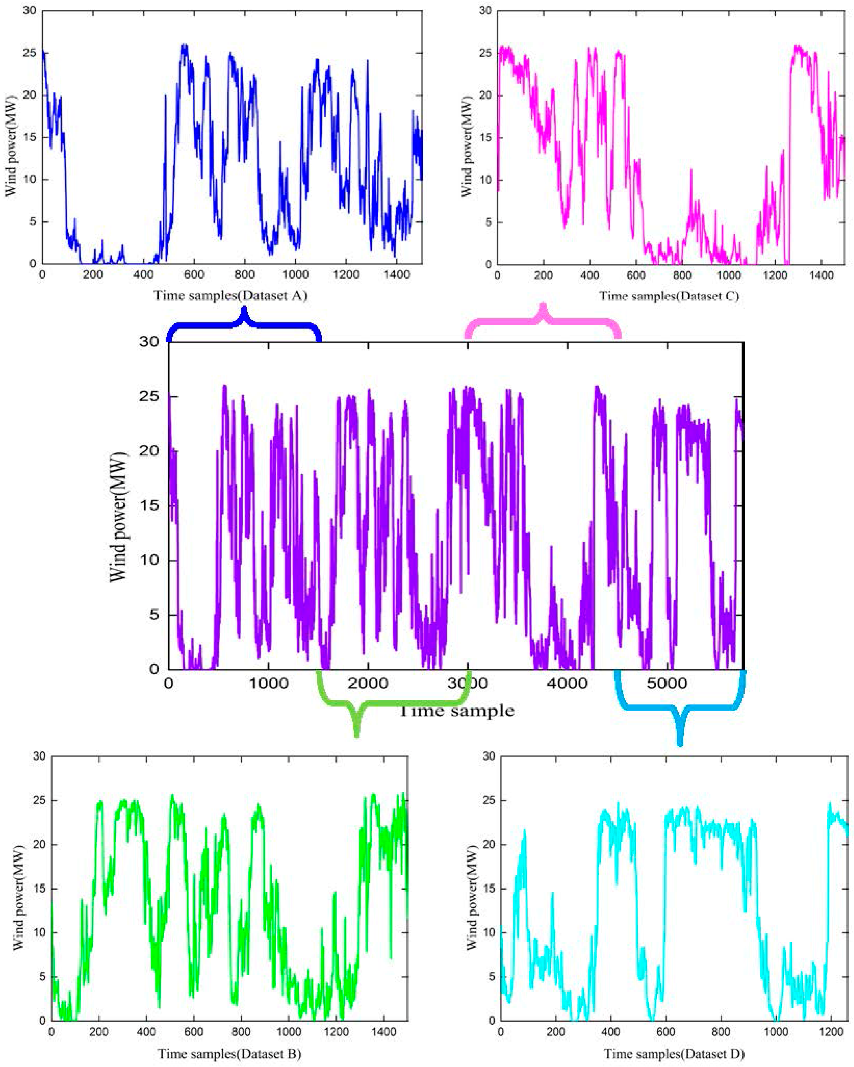
Figure 5.
Decomposition by EEMD of wind power series.

Figure 6.
The permutation entropy values of IMFs.

Figure 7.
Decomposition results by EEMD-PE.
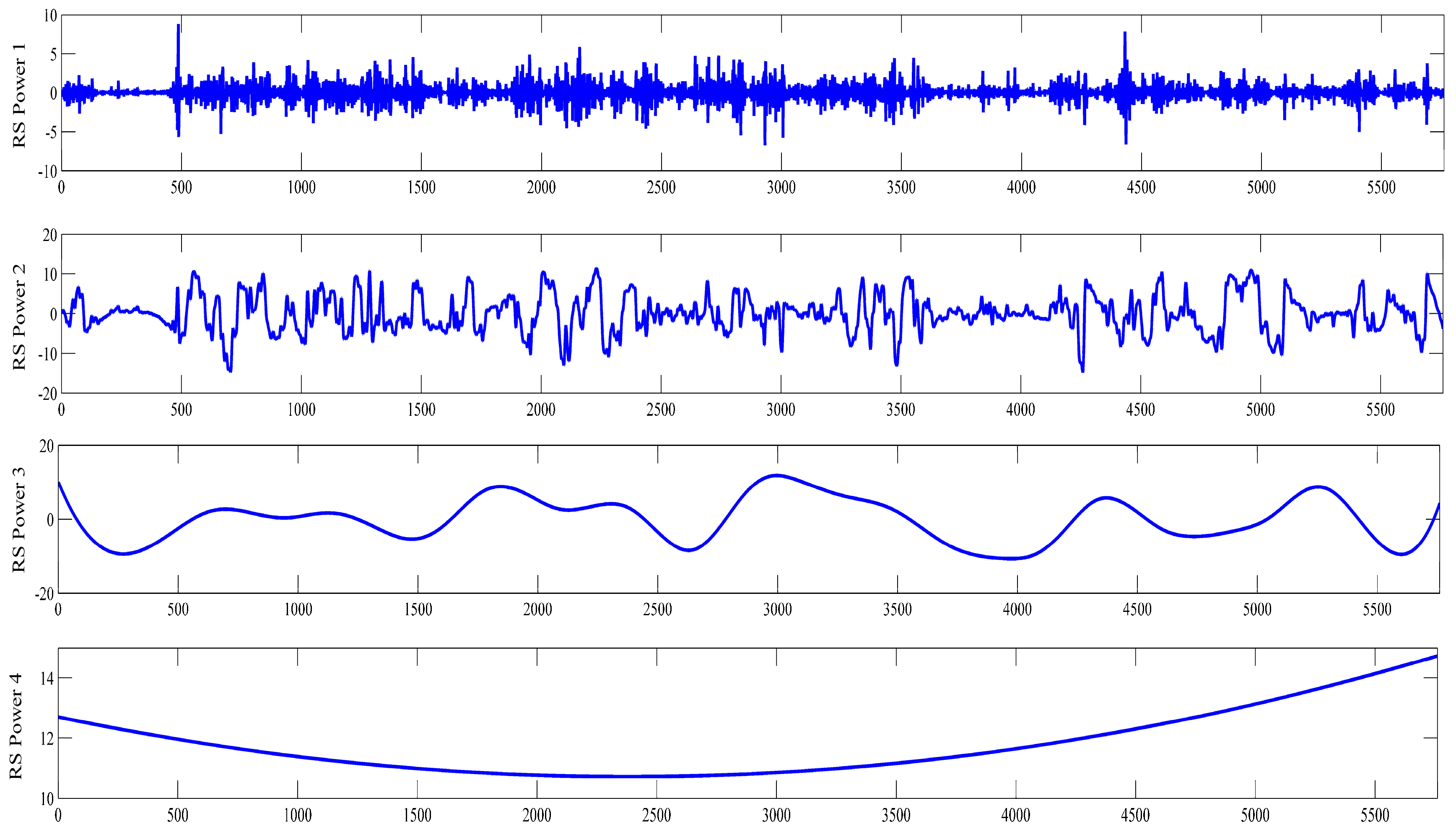
Figure 8.
The NRMSE of 1-step-ahead forecasting by different models with two training datasets.

Figure 9.
Comparison between the forecast and real values for Dataset A. (a) 1-step-ahead result; (b) 4-step-ahead result.
Figure 9.
Comparison between the forecast and real values for Dataset A. (a) 1-step-ahead result; (b) 4-step-ahead result.
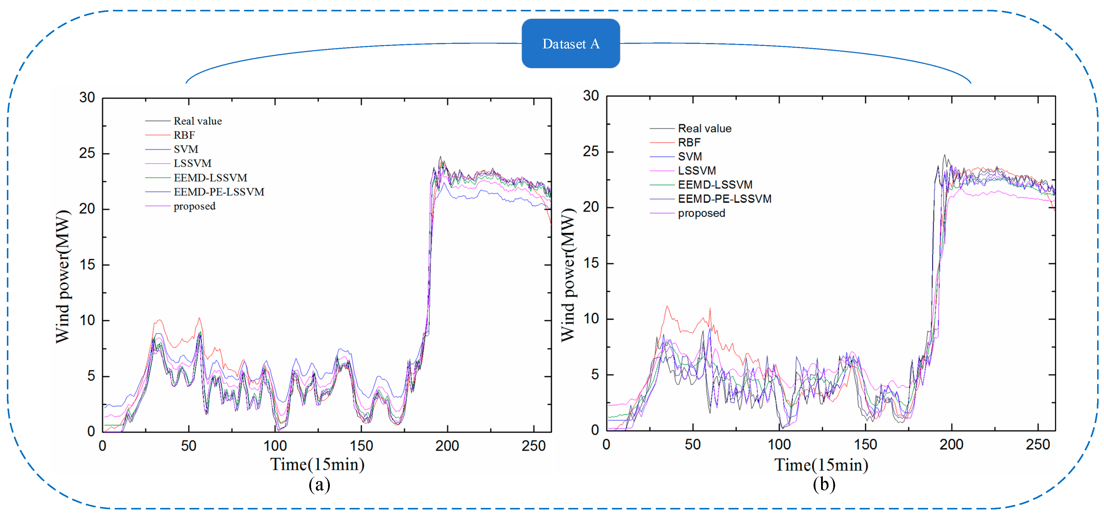
Figure 10.
Comparison between the forecast and real values for Dataset B. (a) 1-step-ahead result; (b) 4-step-ahead result.
Figure 10.
Comparison between the forecast and real values for Dataset B. (a) 1-step-ahead result; (b) 4-step-ahead result.
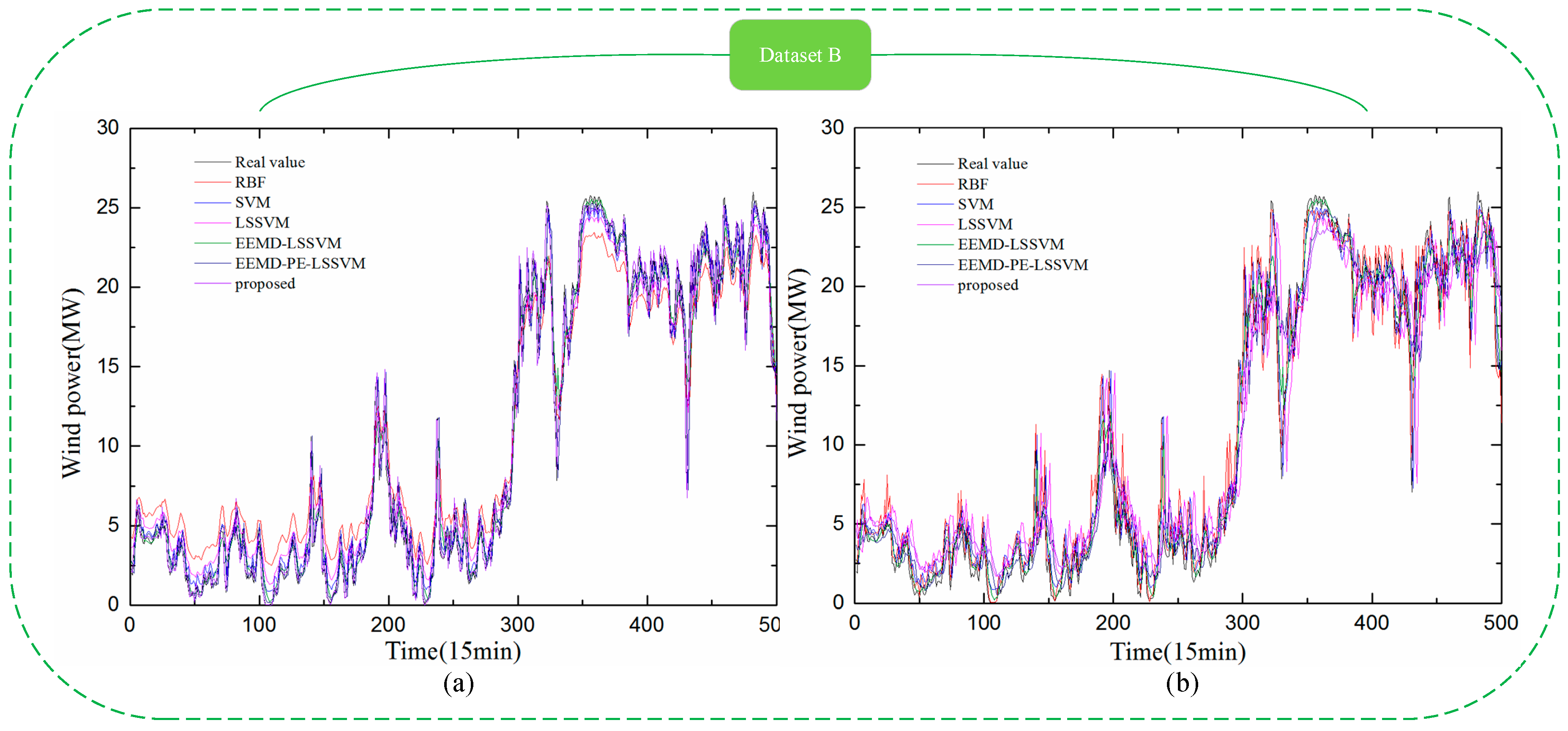
Figure 11.
Comparison between the forecast and real values for Dataset C. (a) 1-step-ahead result; (b) 4-step-ahead result.
Figure 11.
Comparison between the forecast and real values for Dataset C. (a) 1-step-ahead result; (b) 4-step-ahead result.
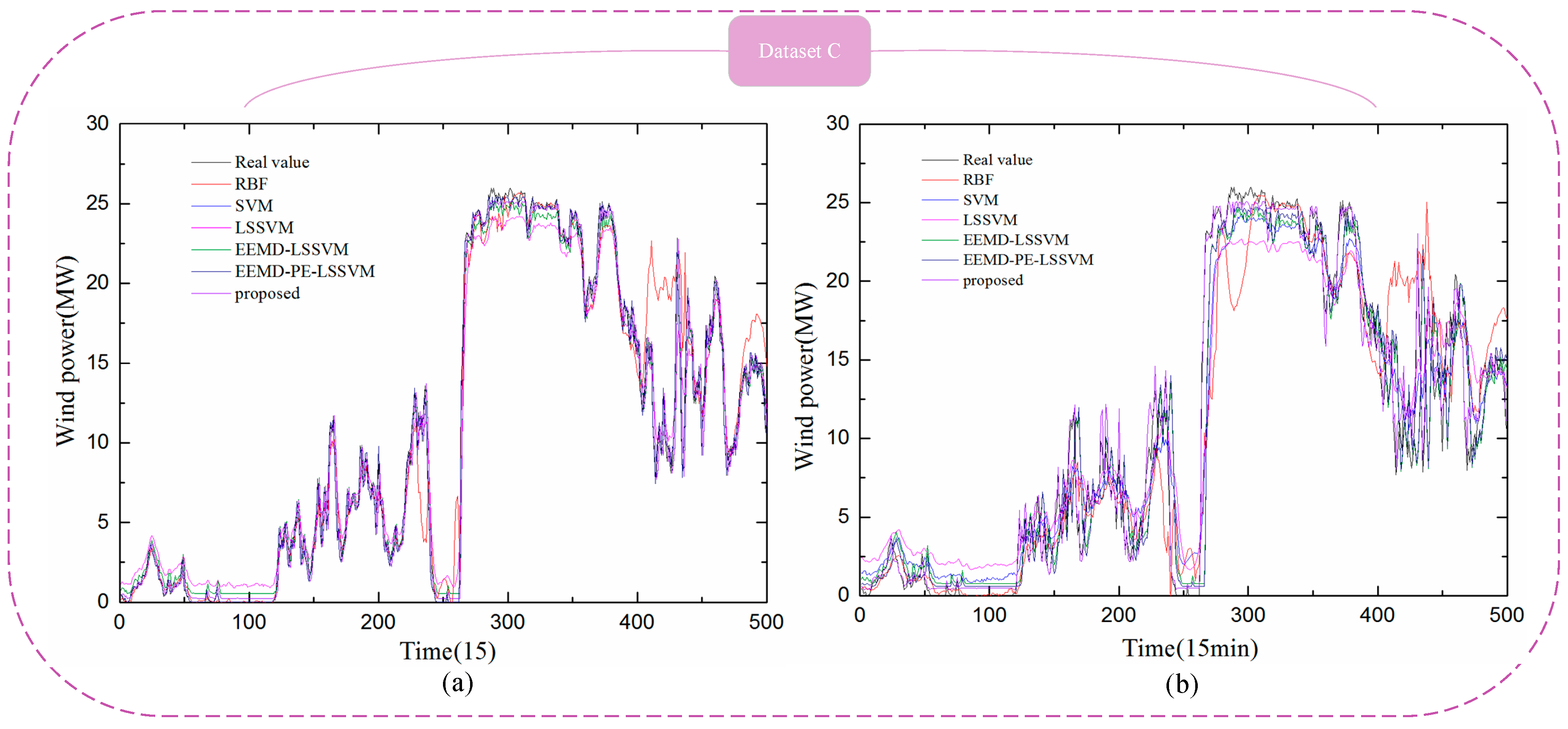
Figure 12.
Comparison between the forecast and real values for Dataset D. (a) 1-step-ahead result; (b) 4-step-ahead result.
Figure 12.
Comparison between the forecast and real values for Dataset D. (a) 1-step-ahead result; (b) 4-step-ahead result.
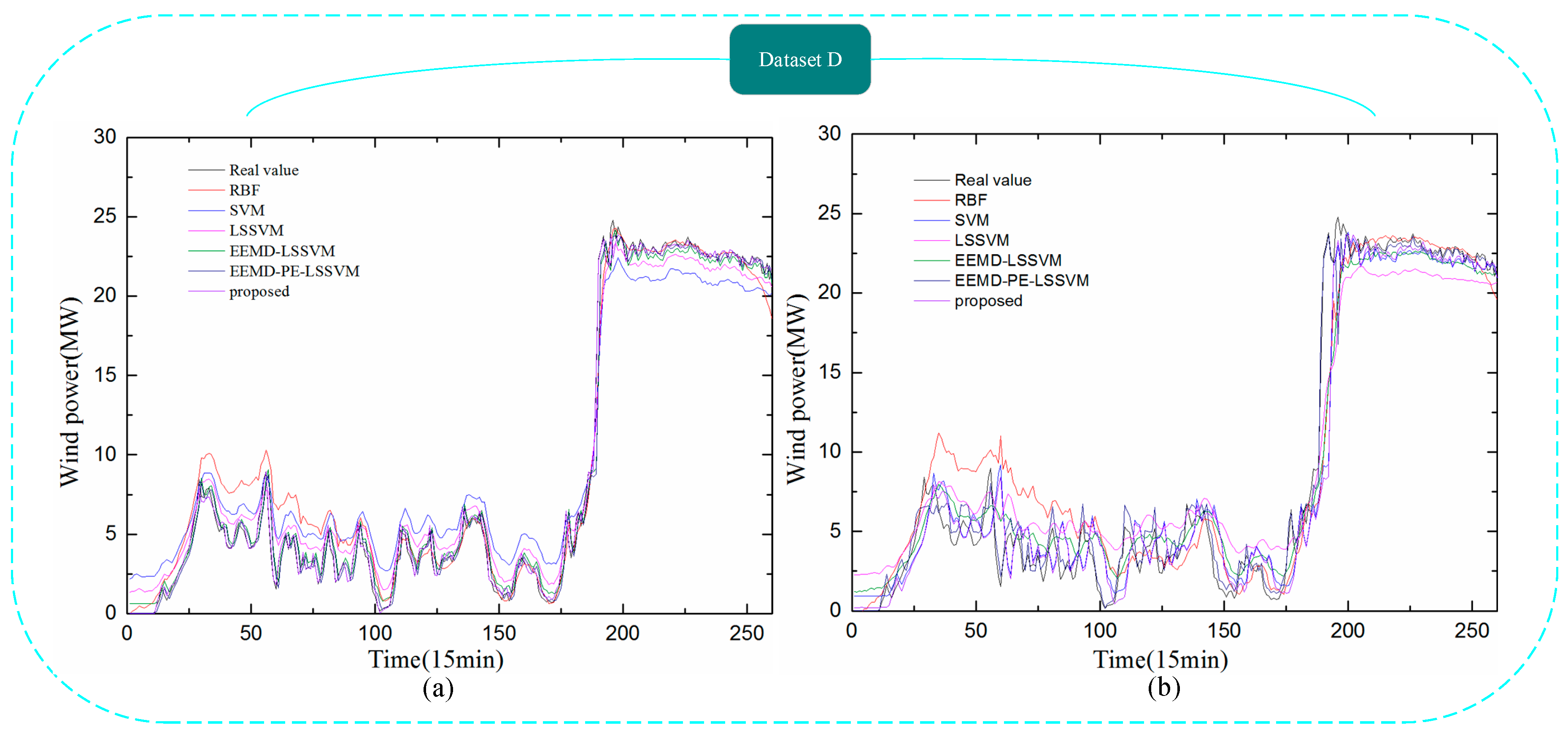
Figure 13.
Histograms of NRMSE and NMAE for all models using Datasets A, B, C, and D, with (1–4)-step-ahead.
Figure 13.
Histograms of NRMSE and NMAE for all models using Datasets A, B, C, and D, with (1–4)-step-ahead.


Table 1.
The NRMSE and NMAE of the testing sample with different values of m and .
| Indicator | NRMSE | NMAE | Modeling Time (s) | NRMSE | NMAE | Modeling Time (s) | NRMSE | NMAE | Modeling Time (s) |
|---|---|---|---|---|---|---|---|---|---|
| 3 | 2.9778 | 1.9901 | 9.9635 | 2.9813 | 1.9601 | 10.1566 | 2.9738 | 1.9601 | 10.7045 |
| 4 | 2.9886 | 1.9783 | 10.3289 | 3.0112 | 1.9605 | 10.2562 | 3.0685 | 1.9978 | 10.0467 |
| 5 | 3.0137 | 1.9644 | 10.5294 | 2.9867 | 1.9384 | 10.3086 | 3.0334 | 1.9824 | 11.7248 |
| 6 | 3.0152 | 1.9735 | 10.4951 | 2.9863 | 1.9583 | 10.3605 | 2.9744 | 1.9463 | 10.5937 |
| 7 | 3.0548 | 2.0172 | 11.0421 | 3.1121 | 1.9858 | 11.6372 | 3.3363 | 2.0956 | 11.8948 |
| average | 3.0100 | 1.9847 | 10.4718 | 3.0078 | 1.9606 | 10.5434 | 3.0773 | 1.9964 | 10.9929 |
Table 2.
Setting the experimental parameters.
| Model | Experimental Parameters | Default Value |
|---|---|---|
| GSA | particle number | 30 |
| maximum evolutionary generation number | 30 | |
| gravitational constant | 100 | |
| attenuation rate | 10 | |
| range of the test function | [0.01, 100] | |
| dimension of the test function | 2 | |
| LSSVM | value range of kernel parameter | [0.01, 10] |
| value range of parameter | [0.1, 1200] | |
| RBFNN | training precision | 0.0001 |
| neuron number of the input layer | 1 | |
| neuron number of the hidden layer | 3 | |
| neuron number of the output layer | 1 |
Table 3.
Optimal kernel function parameters.
| Types of Kernel Function | Penalty Factor | Kernel Function Parameters |
|---|---|---|
| RBF |
Table 4.
The values of NRMSE, NMAE and R for six models in Dataset A.
| Indicator | NRMSE (%) | NMAE (%) | R (%) | |||||||||
|---|---|---|---|---|---|---|---|---|---|---|---|---|
| Time horizon | 1-step | 2-step | 3-step | 4-step | 1-step | 2-step | 3-step | 4-step | 1-step | 2-step | 3-step | 4-step |
| RBF | 6.6432 | 8.3647 | 9.0717 | 10.7424 | 4.3353 | 5.6122 | 6.5253 | 7.6562 | 90.67 | 86.57 | 81.63 | 75.78 |
| SVM | 5.5528 | 7.1953 | 8.6525 | 10.1627 | 4.3245 | 5.5247 | 6.6472 | 7.7864 | 94.87 | 90.72 | 85.89 | 80.20 |
| LSSVM | 6.2582 | 7.8868 | 9.1352 | 10.1816 | 5.0344 | 6.2646 | 7.1246 | 7.8225 | 93.65 | 85.53 | 77.73 | 71.21 |
| EEMD-LSSVM | 5.5714 | 8.4635 | 10.5156 | 12.0235 | 4.1735 | 6.3327 | 7.9133 | 8.9266 | 95.7 | 91.46 | 86.3 | 82.24 |
| EEMD-PE-LSSVM | 4.5363 | 6.9125 | 8.5431 | 9.7176 | 3.3664 | 4.3626 | 5.9448 | 8.9611 | 96.75 | 92.32 | 88.9 | 84.35 |
| Proposed | 4.1884 | 6.7376 | 7.3766 | 9.0113 | 3.1867 | 4.1885 | 5.3326 | 8.6643 | 99.46 | 98.96 | 97.99 | 97.68 |
Table 5.
The values of NRMSE, NMAE and R for six models in Dataset B.
| Indicator | NRMSE (%) | NMAE (%) | R (%) | |||||||||
|---|---|---|---|---|---|---|---|---|---|---|---|---|
| Time horizon | 1-step | 2-step | 3-step | 4-step | 1-step | 2-step | 3-step | 4-step | 1-step | 2-step | 3-step | 4-step |
| RBF | 5.1226 | 6.4646 | 6.9672 | 7.5973 | 3.4726 | 4.5874 | 4.9797 | 5.3514 | 96.05 | 96.19 | 94.46 | 93.44 |
| SVM | 5.6434 | 6.5854 | 7.3128 | 8.3364 | 4.5374 | 5.1553 | 5.6744 | 6.1772 | 94.47 | 96.30 | 95.09 | 93.90 |
| LSSVM | 7.2826 | 8.3536 | 8.7153 | 8.9557 | 6.5156 | 7.2438 | 7.4639 | 7.5716 | 97.9 | 96.32 | 95.3 | 94.61 |
| EEMD-LSSVM | 5.6447 | 8.1175 | 9.3537 | 10.2974 | 4.0737 | 5.7973 | 6.7243 | 7.5343 | 96.62 | 92.88 | 90.56 | 88.58 |
| EEMD-PE-LSSVM | 4.5356 | 6.6436 | 7.8475 | 8.7764 | 3.8383 | 5.7538 | 6.8929 | 7.9927 | 98.25 | 96.22 | 94.76 | 93.36 |
| Proposed | 4.3235 | 6.3164 | 7.5626 | 8.9962 | 2.9927 | 4.5847 | 5.9927 | 6.3338 | 99.81 | 99.49 | 99.42 | 99.26 |
Table 6.
The values of NRMSE, NMAE and R for six models in Dataset C.
| Indicator | NRMSE (%) | NMAE (%) | R (%) | |||||||||
|---|---|---|---|---|---|---|---|---|---|---|---|---|
| Time horizon | 1-step | 2-step | 3-step | 4-step | 1-step | 2-step | 3-step | 4-step | 1-step | 2-step | 3-step | 4-step |
| RBF | 9.4631 | 9.8434 | 9.4552 | 12.1662 | 5.3172 | 5.4662 | 5.6846 | 7.7175 | 92.05 | 87.07 | 87.95 | 83.39 |
| SVM | 4.9958 | 6.2820 | 7.2430 | 8.3250 | 4.0549 | 4.7668 | 5.4573 | 6.1938 | 98.32 | 96.71 | 95.30 | 95.30 |
| LSSVM | 6.7291 | 7.8755 | 8.5629 | 9.4239 | 5.8439 | 6.5553 | 6.9874 | 7.4729 | 98.09 | 95.54 | 94.24 | 92.74 |
| EEMD-LSSVM | 4.3984 | 6.9439 | 8.8273 | 10.2339 | 3.1895 | 4.5649 | 5.6227 | 6.4657 | 98.08 | 95.00 | 91.85 | 89.00 |
| EEMD-PE-LSSVM | 3.4629 | 5.6243 | 7.1929 | 8.3749 | 2.8136 | 4.2865 | 5.4144 | 6.2728 | 99.04 | 97.44 | 95.77 | 94.25 |
| Proposed | 3.9255 | 5.2738 | 6.2736 | 8.1817 | 2.5687 | 4.0292 | 5.2535 | 6.1093 | 99.92 | 99.85 | 99.49 | 99.26 |
Table 7.
The values of NRMSE, NMAE and R for six models in Dataset D.
| Indicator | NRMSE (%) | NMAE (%) | R (%) | |||||||||
|---|---|---|---|---|---|---|---|---|---|---|---|---|
| Time horizon | 1-step | 2-step | 3-step | 4-step | 1-step | 2-step | 3-step | 4-step | 1-step | 2-step | 3-step | 4-step |
| RBF | 5.7482 | 6.6848 | 6.2486 | 9.1483 | 4.0141 | 4.6735 | 4.0979 | 6.2376 | 97.03 | 96.58 | 95.21 | 91.00 |
| SVM | 4.4814 | 5.1492 | 5.7937 | 6.8674 | 3.7321 | 3.9372 | 4.1503 | 4.6592 | 99.03 | 98.11 | 96.95 | 95.49 |
| LSSVM | 6.6836 | 7.1152 | 7.5974 | 8.2797 | 6.1482 | 6.2483 | 6.4237 | 6.7349 | 99.2 | 98.15 | 97.18 | 96.11 |
| EEMD-LSSVM | 3.2975 | 5.6603 | 6.3875 | 7.7385 | 2.2579 | 3.3714 | 4.1872 | 4.8933 | 98.89 | 96.95 | 95.03 | 93.25 |
| EEMD-PE-LSSVM | 3.1542 | 5.2385 | 6.1969 | 7.5508 | 1.9632 | 3.1385 | 3.9653 | 4.6587 | 99.45 | 98.46 | 97.44 | 96.48 |
| Proposed | 2.8432 | 5.1474 | 6.0947 | 6.3749 | 1.1869 | 4.9532 | 4.3978 | 5.9485 | 99.93 | 99.8 | 99.59 | 99.20 |
Table 8.
The simulation time for all methods.
| Approaches | Proposed | EEMD-PE-LSSVM | EEMD-LSSVM | LSSVM | SVM | RBF |
|---|---|---|---|---|---|---|
| Dataset A | 158.4554 | 130.6064 | 129.5019 | 30.4655 | 12.5090 | 14.5357 |
| Dataset B | 158.1473 | 130.3876 | 129.4410 | 30.3430 | 11.6306 | 13.1059 |
| Dataset C | 159.9275 | 132.2656 | 129.4538 | 28.4974 | 12.6486 | 14.9028 |
| Dataset D | 154.4916 | 127.4774 | 126.4261 | 27.3058 | 11.4950 | 12.6474 |
| Average | 157.75545 | 130.18425 | 128.7057 | 29.152925 | 12.0708 | 13.79795 |
© 2018 by the authors. Licensee MDPI, Basel, Switzerland. This article is an open access article distributed under the terms and conditions of the Creative Commons Attribution (CC BY) license (http://creativecommons.org/licenses/by/4.0/).
Share and Cite
MDPI and ACS Style
Lu, P.; Ye, L.; Sun, B.; Zhang, C.; Zhao, Y.; Teng, J. A New Hybrid Prediction Method of Ultra-Short-Term Wind Power Forecasting Based on EEMD-PE and LSSVM Optimized by the GSA. Energies 2018, 11, 697. https://doi.org/10.3390/en11040697
AMA Style
Lu P, Ye L, Sun B, Zhang C, Zhao Y, Teng J. A New Hybrid Prediction Method of Ultra-Short-Term Wind Power Forecasting Based on EEMD-PE and LSSVM Optimized by the GSA. Energies. 2018; 11(4):697. https://doi.org/10.3390/en11040697
Chicago/Turabian StyleLu, Peng, Lin Ye, Bohao Sun, Cihang Zhang, Yongning Zhao, and Jingzhu Teng. 2018. "A New Hybrid Prediction Method of Ultra-Short-Term Wind Power Forecasting Based on EEMD-PE and LSSVM Optimized by the GSA" Energies 11, no. 4: 697. https://doi.org/10.3390/en11040697
Note that from the first issue of 2016, this journal uses article numbers instead of page numbers. See further details here.