Wind Speed Prediction with Spatio–Temporal Correlation: A Deep Learning Approach


1
State Key Laboratory of Advanced Electromagnetic Engineering and Technology, Hubei Electric Power Security and High Efficiency Key laboratory, School of Electrical and Electronic Engineering, Huazhong University of Science and Technology, Wuhan 430074, China
2
Department of Electrical Engineering and Computer Science, University of Tennessee, Knoxville, TN 37996, USA
*
Author to whom correspondence should be addressed.
Energies 2018, 11(4), 705; https://doi.org/10.3390/en11040705
Submission received: 11 February 2018
/
Revised: 4 March 2018
/
Accepted: 20 March 2018
/
Published: 21 March 2018
(This article belongs to the Special Issue Sustainable and Renewable Energy Systems)
Abstract
:Wind speed prediction with spatio–temporal correlation is among the most challenging tasks in wind speed prediction. In this paper, the problem of predicting wind speed for multiple sites simultaneously is investigated by using spatio–temporal correlation. This paper proposes a model for wind speed prediction with spatio–temporal correlation, i.e., the predictive deep convolutional neural network (PDCNN). The model is a unified framework, integrating convolutional neural networks (CNNs) and a multi-layer perceptron (MLP). Firstly, the spatial features are extracted by CNNs located at the bottom of the model. Then, the temporal dependencies among these extracted spatial features are captured by the MLP. In this way, the spatial and temporal correlations are captured by PDCNN intrinsically. Finally, PDCNN generates the predicted wind speed by using the learnt spatio–temporal correlations. In addition, three error indices are defined to evaluate the prediction accuracy of the model on the wind turbine array. Experiment results on real-world data show that PDCNN can capture the spatio–temporal correlation effectively, and it outperforms the conventional machine learning models, including multi-layer perceptron, support vector regressor, decision tree, etc.
1. Introduction
The large-scale integration of wind power poses increasing challenges for the security and economy of power systems due to the intermittent and stochastic nature of wind speed [1,2,3]. Accurate prediction of wind speed and wind power is important for a power system’s peak regulation and frequency adjustment, which are the fundamental requirements for wind power integration into the electrical system [4,5,6,7,8].
Estimating wind power conversion after predicting wind speed benefits the accuracy of wind power prediction, since wind power prediction should take the uncertainties in the process of energy conversion into consideration, such as generation dispatching, equipment maintenance and other social behaviors [9]. Tremendous efforts have been made in the field of wind speed prediction, and dramatic progress has been achieved. However, the majority of the existing work is limited to predicting the wind speed at a certain site by only using the temporal correlation of the time series. As one of the inherent attributes of wind speed at several adjacent positions, the spatial correlation has previously not received enough attention. The spatio–temporal information of wind speed still has great potential for exploitation. With the enrichment of spatio–temporal data of wind farms, wind prediction with both temporal correlation and spatial correlation, i.e., spatio–temporal correlation, has come to the research forefront.
Existing work on wind speed prediction with spatio–temporal correlation can be roughly classified into three categories:
- (1)
- Physical methods, such as numerical weather prediction (NWP)—an accurate technique over longer horizons (from several hours to several days) [10]—formulate the problem of wind speed prediction as a set of high-dimensional, non-linear, differential algebraic equations, according to meteorology and computational fluid dynamics theories. Though physical methods have a good theory base, there are still many factors that limit their application [11], including the demand for considerable computational resources, relatively coarse spatial and temporal resolutions, high dependency for full and accurate information of the environment, etc.
- (2)
- Statistical methods find statistical regularities or patterns in massive historical data by establishing the mapping relationship between the predicted wind speed and explanatory variables [12]. These methods include the time-series analysis method [13], the Kriging interpolation method [14], the augmented Kriging interpolation method [15], clustering analysis [16], Von Mises distribution [17], etc.
- (3)
- Artificial intelligence (AI) methods, inspired by bionics and natural laws, intend to represent the complex nonlinear relationship between the inputs and the outputs. Various methods have been adopted for wind speed prediction, such as artificial neural networks (ANN) [18], support vector regressor (SVR), recurrent neural networks (RNN) [19], etc. However, the majority of the AI methods reported in the literature have shallow architectures and lack a targeted processing mechanism for spatial information. Capturing the temporal dependency and spatial correlation more specifically and pointedly according to their characteristics is a challenging task.
Recent advancements and applications of deep learning provide new thoughts for wind speed prediction. Deep learning fulfills complex learning tasks through constructing learning machines with deep architectures, which has been verified to have a stronger recognition ability for highly nonlinear patterns compared to shallow networks [20]. Deep learning has been widely studied and applied in various frontier fields [21], e.g., computer vision, speech and language processing, Go competition programs, computer virus monitoring, etc. Inspired by these achievements, some attempts have recently been made to employ deep learning techniques for wind speed prediction. For example, Dalto et al. [22] proposed an ultra-short-term wind speed prediction model based on multi-layer neural networks. Zhang et al. [23] and Wang et al. [24] introduced Deep Boltzmann Networks (DBN), a sophisticated deep learning technique for wind speed prediction, while Khodayar et al. [25] proposed two models for ultra-short-term and short-term wind speed prediction based on Stacked Auto-Encoder (SAE). Hu et al. [26] proposed the continuous Restricted Boltzmann Machine (RBM) to predict urban wind speed in Hong Kong. Moreover, Hu et al. [27] and Qureshi et al. [28] discussed the transfer learning technique for a short-term wind speed prediction model with deep neural networks. Though they achieved promising performances, the majority of these methods focus on wind speed prediction for a single site by only using temporal dependencies, instead of taking both spatial and temporal correlations into consideration.
As one of the state-of-the-art deep learning techniques, the convolutional neural network (CNN) has shown a superior ability for automatic spatial feature extraction. The great success of CNN in the field of spatial information processing brings valuable insights for wind speed prediction with spatio–temporal correlation. In this paper, we are concerned with the problem of predicting the wind speed for multiple sites in a wind turbine array simultaneously, instead of at a single site. Initially, the spatial correlation of wind speed at multiple adjacent sites is illustrated from the visualization perspective. A predictive deep convolutional neural network (PDCNN) model for wind speed prediction is proposed, which employs CNNs and the multi-layer perceptron, to capture the spatial and temporal correlations, respectively. Consequently, the whole structure can be seen as a pattern learning model, capable of recognizing a spatio–temporal pattern of wind speed in an end-to-end manner [29]. As a case study, we tested our model with a wind turbine array in Indiana; the results demonstrate that the proposed method for wind speed prediction with spatio–temporal correlation, namely PDCNN, has superior performance.
The main contributions of this paper can be summarized as follows: (1) A new problem—wind speed prediction for multiple sites within a wind turbine array—is solved in this paper. The spatial dimension of wind prediction is expanded from one point to multiple points in 2D space; (2) A two-stage strategy for modeling spatio–temporal sequences is proposed, namely, extracting the spatial features first, followed by capturing the temporal dependencies among the extracted spatial features; (3) A novel deep learning architecture, predictive deep convolutional neural network (PDCNN), is proposed for the wind speed prediction with spatio–temporal correlation. This model captures the spatial and temporal correlation intrinsically, which will contribute to an accurate prediction; (4) Three error indices evaluating the wind speed prediction performance for a wind turbine array are defined.
The rest of this paper is organized as follows: Section 2 analyses the spatial correlation of wind speed from the visualization perspective. Section 3 explains the modeling ideas for spatial–temporal sequence prediction. Section 4 introduces CNN briefly. Section 5 presents a deep learning approach, PDCNN, for wind speed prediction with spatio–temporal correlation. The experimental results are discussed in Section 6. The conclusions are made in Section 7.
2. Spatial Correlation of Wind Speed
2.1. Description with Visualization
The geographical scale is an essential parameter when discussing spatial correlation in wind speed prediction tasks. Large geographical scales are often chosen when the research objects are large-scale wind farm groups. Otherwise, small geographic scales correspond to small-scale objects, such as wind turbines within a wind farm. In this paper, the geographical scale is set to be small to predict the wind speed at the wind turbines’ hub heights in a wind farm.
In a wind farm, the relationships among the wind speeds at upwind sites and downwind sites are usually not simple time-delay relations, due to the influence of multiple factors including wake effect, geostrophic wind, and ground roughness. Moreover, the relative position relationships and the effects of the factors will change significantly when the wind direction changes. Therefore, it is difficult to analyze the wind speed by physical methods. From the machine learning perspective, the wind speed prediction is a pattern recognition problem, i.e., recognizing the hidden patterns from massive spatio–temporal data.
To illustrate the spatial correlation more intuitively, the wind speeds at 100 sites (a 10 × 10 array) are displayed through visualization. Specifically, the normalized wind speed data is transformed to intensity images (of size 10 × 10), where each block corresponds to a certain wind turbine. In this way, the observation at every time point can form an intensity image. Figure 1 shows 12 intensity images of a wind turbine array in one hour with a temporal resolution of 5 min; the deeper the color, the higher the wind speed. For the readability of the images, the edge of the area with high wind speeds is marked in redlines. As the figure shows, the spatial correlation is obvious in this period. On one hand, wind speed at each site is closely related to those at the adjacent sites. On the other hand, the wind speeds of the whole array have some change regularity. For example, the wind directions can be intuitively estimated based on the intensity images. It is worth pointing out that the change regularity of wind speed, observed from intensity images by unaided eyes, may be weak in some periods. Therefore, the change patterns of wind speeds hiding in the spatio–temporal data are expected to be recognized by learning machines.
2.2. Mathematical Description
Suppose our research object over a spatial region is represented by an m × n grid, consisting of m rows and n columns. The location of each site can be described by two-dimensional rectangular coordinates (i,j). The i and j denote the row number and column number, respectively. Generally, the wind speeds at all the sites in an m × n array at the time point, t, can be described by a spatial wind speed matrix, i.e.,
where x(i,j)t denotes the wind speed at the site (i,j) at the time point, t. Further, the wind speed prediction can be described as:
where p(∙) denotes the probability function, is the matrix to be predicted and , , …, are the observed spatial wind speed matrices, namely, historical data. t is the time point of wind speed prediction, and h is the number of historical wind speed matrixes, and k denotes the prediction horizon.
The problem to be investigated in this paper is predicting wind speed for all sites in the array simultaneously by using the wind speed data.
3. Spatio–Temporal Sequence Modeling
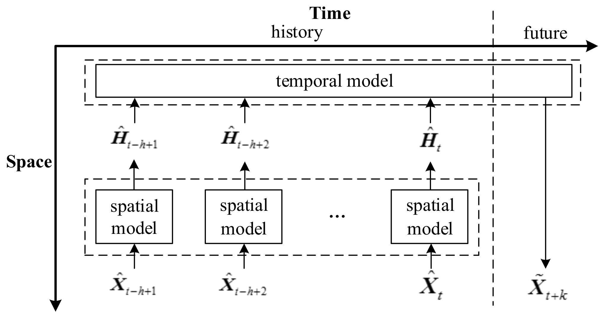
The core of spatio–temporal sequence modeling is taking both spatial correlation and temporal correlation into consideration. In this paper, a two-stage strategy for modeling a spatio–temporal sequence is proposed, namely, extracting the spatial features first, followed by capturing the temporal dependencies among the extracted spatial features. Note that the temporal correlation will not be modeled on raw wind speed data directly, but on the extracted spatial features at h contiguous time points. Figure 2 presents the prediction mode, where spatial feature extraction and temporal dependency capturing are the two key procedures. Under this frame, the whole prediction model should include spatial models and a temporal model to achieve the two key procedures.
In Figure 2, denotes the extracted spatial features.
Wind speeds at the adjacent sites show obvious spatial correlations over the spatial region. For example, the wind speed at the site (i,j) is strongly related to the wind speeds at the sites which are geographically near to (i,j), while it has relatively weak correlations with those at the distant sites. Therefore, to predict the wind speed at one certain site, we are expected to introduce wind speed data of a limited and specific region, instead of the whole array. Due to the spatial correlation of the wind speed, the basic idea of spatial feature extraction is to extract features from each local region and finally to form complete spatial features. In this paper, CNNs are employed as the spatial models.
Under the frame shown in Figure 2, the temporal model can be regarded as a regression machine, whose function is to represent the nonlinear relations, i.e., temporal dependencies, between the inputs (i.e., the spatial features) and outputs (i.e., the predicted wind speeds). Various models have been applied to capture the temporal dependencies of temporal sequences, such as multi-layer perceptron (MLP), support vector regressor (SVR), decision tree (DT), etc. Theoretically, all the above-mentioned models can be used as the temporal model in this task. In practice, the choice of temporal model depends on several aspects, including the structure flexibility and the parameter training mechanism of the whole prediction model, so that the temporal model can coordinate with the spatial models. Therefore, an MLP is employed as the temporal model in this paper.
Following the two-stage modeling strategy, the wind speed prediction problem can be further formulated as:
From the machine learning perspective, the two key procedures, i.e., spatial feature extraction and temporal dependency capture, can be regarded as encoding and decoding, respectively. Therefore, fencoding and gdecoding represent the implicit functions of the spatial models (i.e., CNNs) and the temporal model (i.e., MLP), respectively.
4. Convolutional Neural Networks
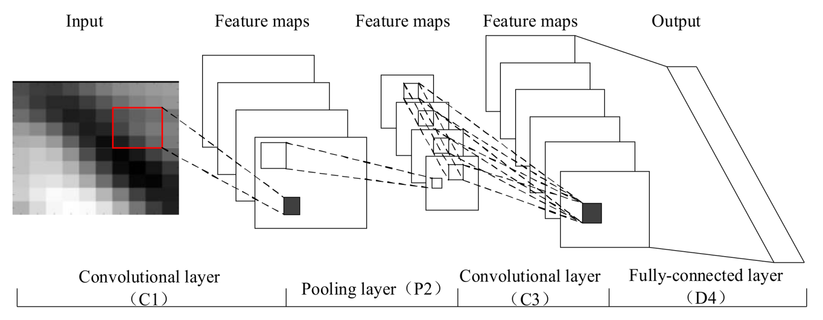
CNN can capture complex spatial features effectively through convolution of multiple convolutional kernels. Figure 3 shows a typical CNN with four layers, including a convolutional layer, a pooling layer, and a fully-connected layer. In typical CNNs, the few layers close to the input are always alternatively convolutional layers and pooling layers. In addition, a few layers close to the output are fully-connected layers. Compared to other deep architectures, CNN has a salient capability for extracting spatial features. In this section, we briefly introduce the structure of a typical CNN.
4.1. Convolutional Layer
The convolutional layer plays a key role in CNN, which is used as a local feature extractor. The input is transformed into feature maps with similar shapes through convolution and nonlinearity at a convolutional layer. The convolution is achieved by several learnable kernels (also named filters), and the nonlinearity is operated by activation functions. Each feature map is a feature representation of the input. In general, the calculation of the convolutional layer can be denoted as:
where * denotes the convolution operation, is the qth feature map of the lth layer, is the trainable convolutional kernel of the lth layer, is the bias matrix, Mq denotes a selection of inputs and f presents the activation function.
Three important strategies are adopted by the convolutional layer to improve the performance of the network—receptive fields, sparse connectivity, and parameter sharing—which can remarkably reduce the number of free variables [30].
4.2. Pooling Layer
The pooling layer yields down-sampled versions of input maps by pooling operation. Firstly, the input map is divided into several non-overlapping rectangular regions with the same size of u × u. Then, the new feature map is computed through summarizing the maximum values or average of the rectangular regions. Suppose there are D input maps, then D new output maps will be generated through the pooling layer. In general, we have:
where down(·) represents a sub-sampling function [31], which will summarize each distinct u-by-u block in the input map, e.g., summation, averaging, and maximizing, etc. According to the computation rule, the size of the output map will be u-times smaller along both spatial dimensions. For example, if the size of the pooling filter is 2 × 2, then the size of the output feature map is reduced to 1/4.
4.3. Fully-Connected Layer
The fully-connected layer is a conventional neural layer, which represents the nonlinear relationships between the input and the output, through activation function and bias. Fully-connected layers are deployed following convolutional layers and sub-sampling layers so as to transform the two-dimensional feature maps to one-dimensional vectors. The data processing procedure can be expressed as:
where wl and bl are the weight matrix and the bias matrix of the fully-connected layer, respectively.
To sum up, the trainable parameters of CNN include convolutional kernel parameters (k), the weight matrix (w), and the bias matrix (b) of the fully-connected layer.
5. The Proposed Model
5.1. The Architecture of the Proposed Model
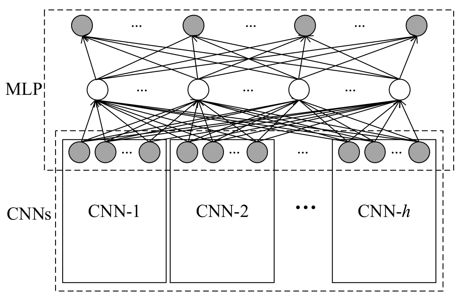
Following the aforementioned two-stage strategy for spatio–temporal sequence modeling, a new deep learning model, named the predictive deep convolutional neural network (PDCNN) is proposed, whose architecture is shown in Figure 4.
PDCNN can be regarded as a multi-branch deep CNN. At the bottom of PDCNN, h CNNs (i.e., CNN-1, CNN-2, …, CNN-h) automatically extract spatial features from the spatial wind speed matrices. On the top of the prediction model, a MLP is built for making predictions for wind speed. In particular, the MLP shares a layer, the input layer, with the CNNs. From the machine learning perspective, the MLP can be regarded as a regression machine, establishing the mapping relationship between the predicted wind speeds (outputs) and the extracted spatial features (inputs) by capturing the temporal dependencies among the extracted spatial features. Consequently, the whole structure can achieve the wind speed prediction with spatio–temporal correlation in an end-to-end manner.
In principle, the structure of each CNN can be set independently. However, in this paper, all CNNs adopt the same structure for convenience. Note that the input layer of the MLP consists of the top layers of the h CNNs. Suppose there are s neurons in the output layer of each CNN, the dimensions of the input layer of the MLP will be s × h. Due to the one-dimensional structure of the output layer of PDCNN, the spatial wind speed matrix cannot be output directly. Thus, a one-to-one correspondence between each element of the spatial wind speed matrix and the neuron in the output layer is built. In this way, the spatial wind speed matrix can be constructed by the output of the prediction model according to the location of the elements. Suppose the wind turbine array consists of m rows and n columns, the dimension of the output layer will be equal to m × n. In addition, the number of other layers and neurons in each layer can be designed flexibly.
5.2. Input Variable Selection
Input variable selection (IVS) has significant impacts on the performance of the models for classification, prediction, etc. For our prediction model, the purpose of IVS is determining the length of the historical sequence fed into the model, i.e., h.
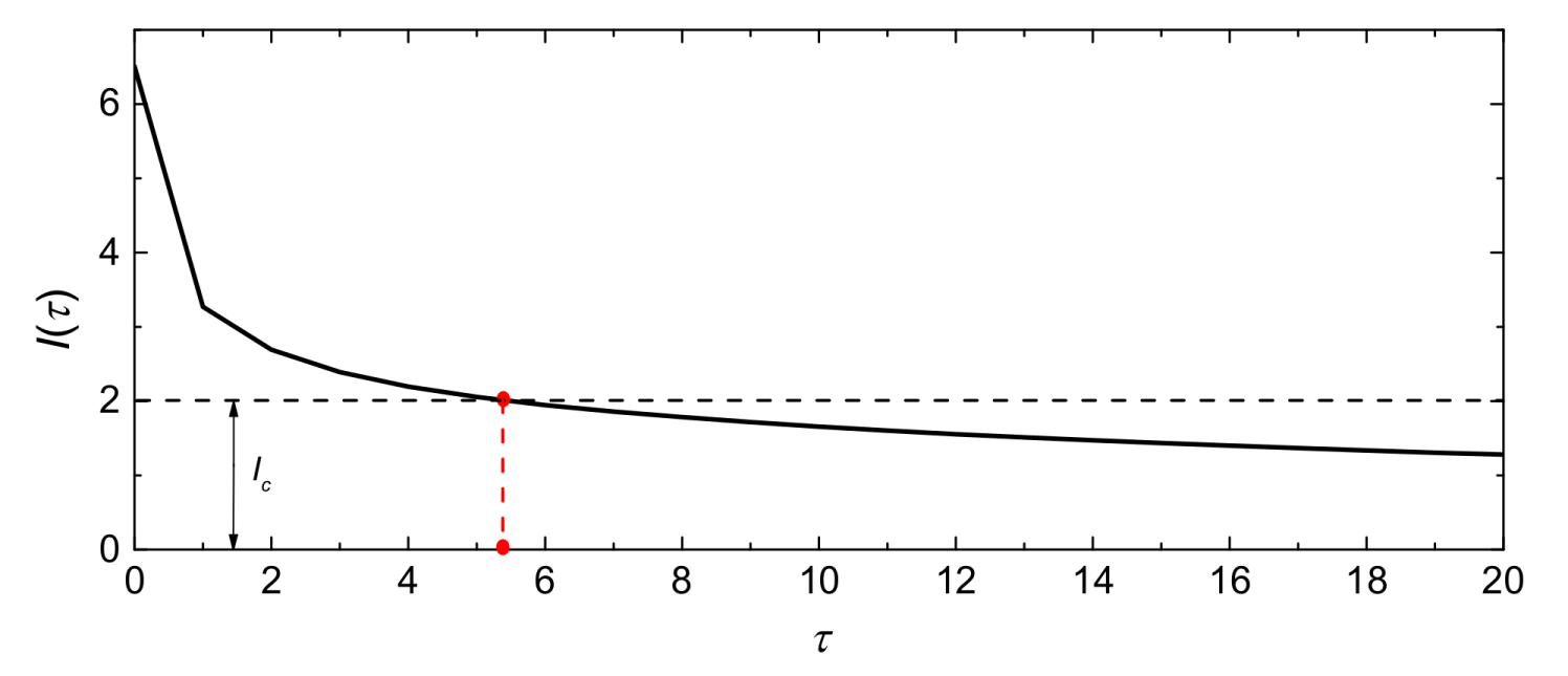
Two pivotal factors—the completeness of the extrapolation knowledge and the scale of the model—should be taken into consideration when determining the value of h. Specifically, with an h that is too small, historical data may lack the extrapolation knowledge required for prediction, whereas the parameter space will be too large, which will likely result in difficulties in parameter optimization. Consequently, there is a trade-off between reducing the scale of the model and maintaining the extrapolation knowledge. In this paper, due to the non-linearity nature of the spatio–temporal sequence, mutual information (MI) [32] is employed for IVS. The MI between two variables measures how much information is known about one variable via the observation of the other variable.
Suppose V(t) and V(t + τ) are the wind speed spatio–temporal sequences at time t and time t + τ, respectively; τ denotes the time-lag. We calculate the MI between V(t) and V(t + τ), represented as I(τ), as the τ changes, to measure the correlations between wind speed spatio–temporal sequences. Figure 5 shows the I(τ)–τ curve with τ from 0 to 20.
Typically, I(τ) is a decreasing function [33]. The input variables can be selected by comparing I(τ) with a threshold (Ic). Namely, h will be equal to the maximum integer of τ whose responding I(τ) > Ic. For example, setting Ic = 2, h will equal 5. Note that the value of the threshold is often set with artificial experience according to the actual situation of the specific task.
5.3. Training Algorithm for PDCNN
Back-propagation (BP) algorithms are able to compute the error for each network layer and can derive learning rules for parameters, so as to make the network outputs close to the target values. There are several commonly used BP algorithms, including stochastic gradient descent (SGD), Adadelta, Adagrad, RMSprop, Adam, etc. In this paper, RMSprop is employed to train the prediction model.
Though PDCNN consists of different kinds of network architectures, including CNNs and MLP, it can be jointly trained with one loss function. In essence, the wind speed prediction problem is a regression problem. Therefore, the mean square error (MSE) function is used as the loss function (also called cost function), denoted as J, in the training process, which is expressed as:
where M is the number of training samples, a(i,j)t and p(i,j)t are the actual and predicted values of wind speed at the site (i,j) at t, respectively.
5.4. Evaluation Indices
Compared to the wind speed prediction for a single site, the wind speed prediction for multiple sites requires more complete evaluation indices. They are expected to not only evaluate the prediction accuracy at every single site but also evaluate the overall prediction performance over the whole spatial region.
In this paper, the mean absolute percentage error (MAPE) εM(i,j) and root mean squared error (RMSE) εR(i,j) are employed to evaluate the prediction accuracy at the site (i,j), which are defined as:
where N denotes the number of the testing samples.
Accordingly, the error indices for the whole array can be defined. εM and εR, named as Array-MAPE (A-MAPE) and Array-RMSE (A-RMSE), respectively, are used to denote the MAPE and RMSE for the whole array, respectively. The two indices are expressed as:
Calculated using εM(i,j) and εR(i,j) for all sites in the array, εM and εR reflect the overall average performance of the prediction model. For a certain time point (t), the prediction error of the model is not the comparison between the two values, but the calculation between the two matrices instead. In this paper, an index, ε(t), is defined, to describe the instantaneous error of the prediction model, which is expressed as:
where ||·||F denotes the Frobenius-norm, and Pt and At are the predicted spatial wind speed matrix and actual spatial wind speed matrix, respectively.
On this basis, the maximum instantaneous error (MIE) is defined, to measure the individual error control ability of the model, which is expressed as:
To sum up, the prediction accuracy for any single site (i,j) is evaluated by εM(i,j) and εR(i,j), and the prediction performance for the whole array is measured by εM, εR, and εMIE. The smaller the values of the indices are, the better the performance of the model is.
6. Case Study
6.1. Database
The National Renewable Energy Laboratory (NREL) provided the Wind Integration National Dataset (WIND) [34], which contains wind speed data for more than 126,000 sites in the continental United States for the years 2007–2013. Based on this data source, this paper selected a 10 × 10 wind turbine array in Indiana (85.1855W, 40.4092N) as the research object, as shown in Figure 6. The wind speed data of the array collected in the first quarter of 2012, i.e., from January to March, wais selected, which includes 25,920 frame data with 5-min time resolution. The maximum wind speed is 27.228 m/s, and the minimum wind speed is 0.048 m/s.
The dataset was divided into three subsets, namely the training set (60%), validation set (20%), and testing set (20%). Specifically, the training set consisted of the first 15,552 frame data, the validation set consisted of the following 5184 frame data, and the testing set consisted of the remaining 5184 frame data. The training set and testing set served as models for training and testing, respectively. The validation set is used to compare different models and choose a better one [25]. Moreover, the MSE (defined as Equation (7)) on the validation set, i.e., validation error, was monitored during the training process. That the validation error decreased during the training process indicated the model did not suffer from overfitting.
6.2. Model Configuration and Implement Details
Determining the optimal structures of different deep-learning models for different problems is still an open issue [23]. For the DPCNN, the structure parameter space can be very large due to its deep architecture. In this paper, the structure of the model was determined by the combination of artificial experience and machine searching.
Specifically, considering the short prediction horizons (i.e., from 5 min to 1 hour) in this paper, the length of the input spatio–temporal sequence, i.e., the number of CNNs in PDCNN, was set to be 5 according to the mutual information in Figure 5. The 5 CNNs adopted the same structure. Specifically, each CNN had 4 layers: (1) a convolutional layer, C1, with 10 filters with a respective field of 3 × 3; (2) a pooling layer, P2, with a pooling size of 2 × 2 (the pooling layer applied max-pooling); (3) a convolutional layer, C3 ,with 30 filters, with a receptive field of 4 × 4; (4) a fully-connected layer, D4, with 30 neurons. Two fully-connected layers, D5 and D6, were designed to capture the temporal dependencies among the outputs of the 5 CNNs. There were 100 neurons in D6, which equals the number of turbines in the array. The number of neurons in D5, denoted as a, was selected from the set Φ = {100, 200, 300, 400}. The architecture of the proposed PDCNN was shown in Figure 7.
C1, C3, D4 and D5 adopted the rectified linear unit (ReLU)—a notable non-saturated activation function—as their activation functions, according to the empirical success of ReLU applied in deep CNN [35] and deep belief networks (DBN) [36]. D6 employed a sigmoid function as the activation function so as to protect the output layer from sparsity which results in the outputs of some neurons being equal to zero. Moreover, all the parameters of PDCNN were initialized randomly. In order to reduce over-fitting, the dropout, an effective technique to fight against over-fitting, was applied only to the fully-connected layer, D5, since dropout is far less advantageous in convolutional layers [37]. In this paper, we opted to utilize dropout with a probability of 0.5. The PDCNN was trained with RMSprop with a mini-batch size of 200, and with a custom setting, namely, weight decay ρ = 0.9, learning rate η = 0.001, and fuzz factor ε = 10−6. The epochs for training was set to 100.
We implemented the network with the Keras framework using Theano [38] backend. Experiments were carried out on a 64-bit PC with Inter core i7-7820 CPU/32.00GB RAM.
6.3. Baseline Algorithms
Four popular algorithms for time series prediction were used as the baseline algorithms, including one statistic algorithm, i.e., the persistence method (PR), and three machine-learning algorithms with shallow architecture, namely, MLP, SVR, and DT.
PR, a simple method for ultra-short-term prediction, uses a simple assumption that the predicted data is the same as the data in present time. MLP has three layers, whose dimensions of the input layer and output layer are 500 and 100 respectively. MLP adopts ReLU in the input layer and the hidden layer and sigmoid in the output layer. Meanwhile, a dropout with a probability of 0.5 is also applied to the hidden layer to prevent over-fitting. Moreover, MLP is trained with Adam with the learning rate and the number of epochs is set to 0.001 and 100, respectively. The only hyper-parameter (i.e., parameters that are not directly learnt with estimators) to be explored for MLP is the dimension of the hidden layer, denoted as b, which will be selected from {100, 200, 300, 400, 500, 600, 700, 800, 900, 1000}. SVR adopts the radial basis function (RBF) as the kernel function due to its high generalization capability [39]. The two hyper-parameters in SVR to be determined are γ ∈ {2−2, 2−1, 20, 21, 22, 23, 24} and C ∈ {0.1, 1, 10, 100, 1000}. DT uses the CART algorithm. The maximum depth of the tree, a hyper-parameter denoted as e, is selected from {3, 4, 5, 6, 7, 8}.
All of these four baseline algorithms were run on Python (V3.6).
6.4. Performance Analysis
To evaluate the performance of the five models, i.e., the proposed DPCNN and the four baseline algorithms—the experiments with the prediction horizon ranging from 5 min to 1 h (i.e., k ranges from 1 to 12)—were implemented. Namely, all the models were expected to predict the spatial wind speed matrix, , by using the previous 5 spatial wind speed matrices: , , , , . Note that, in contrast to PDCNN, the three baselines (MLP, SVR, and DT) cannot receive 2D matrices directly, which are fed with 1D vectors that are flattened by the spatial wind speed matrices.
All five models were trained and validated with the same training set and validation set, respectively. For each prediction horizon, the hyper-parameters of the models were explored by a grid search. Specifically, with each hyper-parameter choice, a corresponding model was trained using the training set. The validation error was computed after the training process of each model. Finally, the hyper-parameters were determined based on the performance on the validation set. The model with the optimal hyper-parameters yields the lowest validation error. The hyper-parameters of the models are listed in Table 1. The prediction performance of the models with the optimal hyper-parameters was evaluated on the testing set with the three indices, i.e., εM, εR, and εMIE. The results are shown in Table 2, Table 3 and Table 4, respectively.
As the experiment results show in the tables, the proposed DPCNN consistently outperforms the other four baseline models, since it produces the lowest error indices with each prediction horizon (from 5 min to 1 h) compared to others, while PR yields the worst results compared to other models, especially with longer prediction horizons. With the extension of the prediction horizon, the error indices of the five models roughly increase. The average εM, εR and εMIE of PDCNN are 7.14%, 0.728 and 25.956, respectively, and show improvements of 27%, 16% and 13% over multiple prediction horizons compared to MLP, respectively. Meanwhile, PDCNN improved the average εM, εR and εMIE by 29%, 18% and 8% compared to SVR, and by 28%, 18% and 23% compared to DT. This demonstrates that PDCNN shows superiority, not only in the overall average performance, but also in the individual error control ability, compared to the other four baseline models.
Moreover, compared to MLP and DT, SVR has higher εM and εR but lower εMIE, which shows its weaker overall average performance but stronger individual error control ability. This is mainly because MLP and DT are the empirical risk minimization models, whose training processes aim to pursue the best fits on the training data. As a result, there may be cases where the individual error is significant in testing data. In contrast, SVR is a structural risk minimization model, which can avoid this situation to a certain extent. Therefore, SVR has stronger individual error control ability than MLP and DT. Compared to the baseline models, PDCNN handles the spatio–temporal information in a more targeted way. Taking the MLP as an example, in contrast to PDCNN, MLP adopts the single-hidden-layer structure, which employed 500 common neurons as the input layer instead of the five CNNs in PDCNN. Although spatio–temporal information is introduced in this way, the role of spatial correlation is weakened. The different prediction performances yielded by PDCNN and MLP show the effectiveness of the spatio–temporal information processing mechanism of DPCNN. This is mainly because the motion of wind speed is highly correlated in a local spatial region. However, the ordinary fully-connected structure of MLP has too many redundant connections, which is unlikely to capture these spatial correlations [40]. In contrast, the locally-connected structure in DPCNN is able to capture the spatial correlation of wind speed. Therefore, DPCNN shows superiority over MLP.
To further illustrate the spatial correlation processing ability of PDCNN, a prediction model for a single site, based on MLP with three layers, named the local MLP (l-MLP), was employed. Different from the aforementioned baselines, l-MLP is a single-output MLP, which uses the five previous data points to predict the wind speed in the future. The wind speed at each site is predicted by an l-MLP independently; consequently, the prediction result for the whole array can be formed. Therefore, the dimensions of the input layer and output layer are 5 and 1, respectively, while the dimension of the hidden layer is a hyper-parameter to be selected from {50, 60, 70, 80, 90, 100, 150, 200}. The methods for determining the hyper-parameter, the optimizer, and the activation function of each l-MLP are the same as those of the baseline MLP, mentioned above. The prediction results producing by l-MLPs are shown in Table 5.
The results demonstrate that PDCNN outperforms l-MLP, with average improvements of 39%, 30% and 30% in εM, εR and εMIE, respectively. l-MLP is inferior to the other four artificial-intelligence prediction models, including PDCNN, MLP, SVR and DT, in terms of εMIE. This is mainly because l-MLP does not using spatial correlation, as the above four do. At each site, the wind speed is predicted independently, which cannot minimize the error of the whole spatial wind speed matrix. With smaller prediction horizons, the l-MLP yields relatively small εM and εR, which shows a good overall error control ability of l-MLP. For example, in the 5-min ahead prediction tasks, the εM and εR of l-MLP are even lower than those of MLP. In contrast, with the longer prediction horizons, the l-MLP is far less effective in terms of εM and εR. Intuitively, the advantage that PDCNN has over l-MLP becomes bigger with the extension of the prediction horizon. This is mainly a benefit of the hierarchical architecture of DPCNN for utilizing spatial correlation information. Specifically, in PDCNN, the spatial correlation in each spatial correlation domain will be captured by convolution operations initially, and will be transmitted to the higher layer where the more complex features will be formed with the information from more spatial correlation domains. In this way, the wind speed prediction for any site involves not only the neighborhood sites adjacent to this site but also other sites in the array. In contrast, in the l-MLP, the mapping relationship between the output (predicted wind speed) and input (the historical data at this site) is only built on the information at one certain site. Therefore, spatial correlations hidden in the combination of motion over multiple spatial correlation domains is effectively captured by DPCNN.
6.5. Computational Complexity
The time complexity of the learning algorithm includes two aspects, namely, training time complexity and testing time complexity. With the 12 different prediction horizons, the average times for training PDCNN, MLP, SVR, and DT are 106.722 s, 5.526 s, 24.880 s, and 10.169 s, respectively. Note that all the experiments were carried out on the PC illustrated in Section 6.2. The average testing times for MLP and DT are 0.051 s and 0.018 s, respectively, which can be negligible due to the simple feed-forward algorithms used for producing the outputs [25]. DPCNN and SVR take more time for testing, since DPCNN contains max-pooling operations and SVR contains kernel function calculations. The average testing times for PDCNN and SVR are 0.252 s and 6.472 s respectively. That is to say, it only takes PDCNN 0.049 ms for each predicted sample. The reason for the less time needed for testing in PDCNN than SVR is that the complexity of max-pooling operation is far less than kernel function calculation. From the perspective of application, the training time is within an acceptable range.
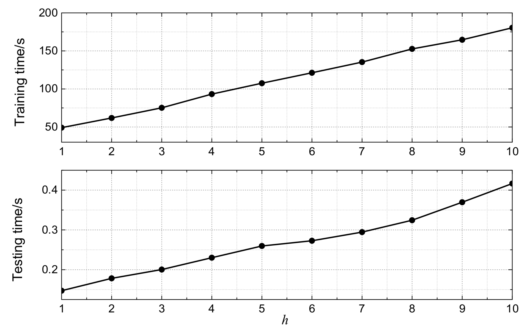
Furthermore, for PDCNN, the central issue to the time complexity is the number of the CNNs employed in the model, h. Figure 8 shows the times for training and testing for PDCNN, with h ranging from 1 to 10 in the 5-min ahead prediction task. Obviously, there is an approximately linear dependency between the time complexity and h, which mainly results from two reasons. The first is that all CNNs have the same number of parameters due to their identical structures. The second is that, during the back-propagation optimization process, each CNN receives the error from the second top layer (D5) and optimizes its parameters independently. It should be noted that the linear dependency indicates the good expansibility of PDCNN.
6.6. Discussion
There are still several open problems, including model selection and computational complexity, for the PDCNN that need to be considered.
Model selection is a universal problem for almost all deep learning models. For PDCNN, the purpose of model selection is to determine the optimal hyper-parameters, such as the number of layers, the dimension of each layer, the size of the receptive fields, the learning rate, etc. Due to the huge hyper-parameter space, employing an exhaustive grid search to explore the optimal combination for the whole hyper-parameter space is impractical. In this paper, some of the hyper-parameters were determined by artificial experience, which can significantly reduce the time and search space explored by the machine. However, this may limit the prediction performance of PDCNN. Therefore, it is worth making a considerable effort to develop the effective machine search method for model selection.
As a model with deep architecture, PDCNN has a higher time complexity compared to conventional models. Although it takes more time to train PDCNN, it is still worth employing PDCNN for wind speed prediction, since it considerably outperforms other models. This may also be a feasible method from a computational point of view, particularly in light of new developments in computer architecture, such as Graphics Processing Units (GPUs) [41] and multicore systems [42]. Employing GPUs to speed up PDCNN will enhance its practicality, which will be the focus of our future work.
7. Conclusions
To further explore the value of spatio–temporal data of wind farms, and enhance the prediction accuracy of wind speed, a novel deep neural network architecture for wind speed prediction with spatio–temporal correlation, PDCNN, was presented in this paper. This model integrates CNNs and the MLP into a unified framework, which takes the advantages of both CNN and MLP. PDCNN is able to achieve spatial correlation extraction and temporal dependency capture simultaneously, which contributes to accurate wind speed prediction. The experiment results on real-world data demonstrate that PDCNN achieves a superior and competitive performance compared to conventional wind prediction models, including MLP, SVR, and DT.
This paper tentatively explores the possibility of applying the deep learning model to wind speed prediction with spatio–temporal correlation, which provides new ideas for research in this field. On this basis, how to make use of more abundant input data, such as temperature and humidity, and how to make a more comprehensive and scientific evaluation of the model’s prediction accuracy will be further explored and studied.
Acknowledgments
This work was supported by the National Key Research and Development Program of China (2016YFB0900100) and the China Scholarship Council. The authors would like to give special thanks to Xiang Bai, and Baoguang Shi from the School of Electronic Information and Communication, Huazhong University of Science and Technology, for their help on experiment implementations.
Author Contributions
Qiaomu Zhu and Jinfu Chen designed the model and conducted the experiments; Lin Zhu analyzed the data; Xianzhong Duan and Yilu Liu edited and improved the manuscript.
Conflicts of Interest
The authors declare no conflict of interest.
References
- Ronay, A.; Olga, F.; Enrico, Z. Two machine approaches for short-term wind speed time-series prediction. Energy Procedia 2011, 12, 770–778. [Google Scholar] [CrossRef]
- Wang, Y.; Zhang, N.; Kang, Q.; Xia, Q. An efficient approach to power system uncertainty analysis with high-dimensional dependencies. IEEE Trans. Power Syst. 2018. [Google Scholar] [CrossRef]
- Wang, X.; Guo, P.; Huang, X. A review of wind power forecasting models. IEEE Trans. Neural Netw. 2016, 27, 1734–1746. [Google Scholar] [CrossRef]
- Zhu, Q.; Chen, J.; Duan, X.; Sun, X.; Li, Y.; Shi, D. A Method for Coherency Identification Based on Singular Value Decomposition. In Proceedings of the IEEE Power and Energy Society General Meeting (PESGM), Boston, MA, USA, 17–21 July 2016; pp. 1–5. [Google Scholar] [CrossRef]
- Ren, Y.; Suganthan, P.N.; Srikanth, N. A Comparative Study of Empirical Mode Decomposition-Based Short-Term Wind Speed Forecasting Methods. IEEE Trans. Sustain. Energy 2015, 6, 236–244. [Google Scholar] [CrossRef]
- Lowery, C.; O’Malley, M. Impact of wind forecast error statistics upon unit commitment. IEEE Trans. Sustain. Energy 2012, 3, 760–768. [Google Scholar] [CrossRef]
- Ju, W.; Sun, K.; Qi, J. Multi-layer interaction graph for analysis and mitigation of cascading outrages. IEEE J. Emerg. Sel. Top. Circuits Syst. 2017, 7, 239–249. [Google Scholar] [CrossRef]
- Ju, P.; Li, H.; Gan, C.; Liu, Y.; Yu, Y.; Liu, Y. Analytical Assessment for Transient Stability Under Stochastic Continuous Disturbances. IEEE Trans. Power Syst. 2018, 33, 2004–2014. [Google Scholar] [CrossRef]
- Damousis, I.G.; Alexiadis, M.C.; Theocharis, J.B.; Dokopoulos, P.S. A fuzzy model for wind speed prediction and power generation in wind parks using spatial correlation. IEEE Trans. Energy Convers. 2004, 19, 352–361. [Google Scholar] [CrossRef]
- Chen, N.; Qian, Z.; Nabney, I.T.; Meng, X. Wind Power Forecasts Using Gaussian Processes and Numerical Weather Prediction. IEEE Trans. Power Syst. 2014, 29, 656–665. [Google Scholar] [CrossRef]
- Soman, S.S.; Zareipour, H.; Malik, O.; Mandal, P. A review of wind power and wind speed forecasting methods with different time horizons. In Proceedings of the North American Power Symposium, Arlington, TX, USA, 26–28 September 2010; pp. 1–8. [Google Scholar] [CrossRef]
- Ding, Y.; Zhou, H.; Tan, Z.; Chen, Y.; Ding, J. The influence of wind direction on short-term wind power prediction: A case study in north China. In Proceedings of the IEEE PES Innovative Smart Grid Technologies, Tianjin, China, 21–24 May 2012; pp. 1–5. [Google Scholar] [CrossRef]
- Ulrich, F.; Matthias, L.; Kai, M.; Mönnich, K.; Waldl, H.; Beyer, H.G.; Luig, A. Short-term prediction of the aggregated power output of wind farms—A statistical analysis of the reduction of the prediction error by spatial smoothing effects. J. Wind Eng. Ind. Aerodyn. 2002, 90, 231–246. [Google Scholar]
- Cellura, M.; Cirrincione, G.; Marvuglia, A. Wind speed spatial estimation for energy planning in Sicily: Introduction and statistical analysis. Renew. Energy 2008, 33, 1237–1250. [Google Scholar] [CrossRef]
- Hur, J.; Baldick, R. Spatial prediction of wind farm outputs using the Augmented Kriging-based Model. In Proceedings of the IEEE Power and Energy Society General Meeting, San Diego, CA, USA, 22–26 July 2012. [Google Scholar] [CrossRef]
- Kusiak, A.; Li, W. Short-term prediction of wind power with a clustering approach. Renew. Energy 2010, 35, 2362–2369. [Google Scholar] [CrossRef]
- Carta, J.A.; Bueno, C.; Ramírez, P. Statistical modeling of directional wind speeds using mixtures of von Mises distributions: Case study. Energy Convers. Manag. 2008, 49, 897–907. [Google Scholar] [CrossRef]
- Bechrakis, D.A.; Sparis, P.D. Correlation of wind speed between neighboring measuring stations. IEEE Trans. Energy Convers. 2004, 19, 400–406. [Google Scholar] [CrossRef]
- Barbounis, T.G.; Theocharis, J.B. Locally recurrent neural networks optimal filtering algorithms: Application to wind speed prediction using spatial correlation. In Proceedings of the 2005 IEEE International Joint Conference on Neural Networks, Montreal, QC, Canada, 31 July–4 August 2005; pp. 2711–2716. [Google Scholar] [CrossRef]
- Bengio, Y. Learning deep architectures for AI. Found Trends Mach. Learn. 2009, 2, 1–127. [Google Scholar] [CrossRef]
- Lemley, J.; Bazrafkan, S.; Corcoran, P. Deep learning for consumer devices and services: Pushing the limits for machine learning, artificial intelligence, and computer vision. IEEE Consum. Electron. Mag. 2017, 6, 48–56. [Google Scholar] [CrossRef]
- Dalto, M.; Matuško, J.; Vašak, M. Deep neural networks for ultra-short-term wind forecasting. In Proceedings of the 2015 IEEE International Conference on Industrial Technology (ICIT), Seville, Spain, 17–19 March 2015; pp. 1657–1663. [Google Scholar] [CrossRef]
- Zhang, C.Y.; Chen, C.L.P.; Gan, M.; Chen, L. Predictive Deep Boltzmann Machine for Multiperiod Wind Speed Forecasting. IEEE Trans. Sustain. Energy 2015, 6, 1416–1425. [Google Scholar] [CrossRef]
- Wang, H.; Wang, G.; Li, G.; Peng, J.; Liu, Y. Deep belief network based deterministic and probabilistic wind speed forecasting approach. Appl. Energy 2016, 182, 80–93. [Google Scholar] [CrossRef]
- Khodayar, M.; Kaynak, O.; Khodayar, M.E. Rough Deep Neural Architecture for Short-term Wind Speed Forecasting. IEEE Trans. Ind. Inform. 2017, 13, 2770–2779. [Google Scholar] [CrossRef]
- Hu, Y.; You, J.; Liu, J.N.K.; Chan, P.W. Continuous RBM Based Deep Neural Network for Wind Speed Forecasting in Hong Kong. In Proceedings of the International Conference on Image Processing, Computer Vision, and Pattern Recognition (IPCV), Las Vegas, NV, USA, 27–30 July 2015; pp. 368–374. [Google Scholar]
- Hu, Q.; Zhang, R.; Zhou, Y. Transfer learning for short-term wind speed prediction with deep neural networks. Renew. Energy 2016, 85, 83–95. [Google Scholar] [CrossRef]
- Qureshi, A.; Khan, A.; Zameer, A.; Usman, A. Wind Power Prediction using Deep Neural Network based Meta Regression and Transfer Learning. Appl. Soft Comput. 2017, 58, 742–755. [Google Scholar] [CrossRef]
- Shi, B.; Bai, X.; Yao, C. An End-to-End Trainable Neural Network for Image-Based Sequence Recognition and Its Application to Scene Text Recognition. IEEE Trans. Pattern Anal. Mach. Intell. 2017, 39, 2298–2304. [Google Scholar] [CrossRef] [PubMed]
- Feng, J.; Li, F.; Lu, S.; Liu, J.; Ma, D. Injurious or noninjurious defect identification from MFL images in pipeline inspection using convolutional neural network. IEEE Trans. Instrum. Meas. 2017, 66, 1883–1892. [Google Scholar] [CrossRef]
- Bouvrie, J. Notes on Convolutional Neural Networks. MIT CBCL Technical Report. 2006. Available online: http://copyrights.org/5869/1/cnn_tutorial.pdf (accessed on 10 Dec 2007).
- Trappenberg, T.; Ouyang, J.; Back, A. Input variable selection: Mutual information and linear mixing measures. IEEE Trans. Knowl. Data Eng. 2006, 18, 37–46. [Google Scholar] [CrossRef]
- Hu, Q.; Su, P.; Yu, D.; Liu, J. Pattern-Based Wind Speed Prediction Based on Generalized Principal Component Analysis. IEEE Trans. Sustain. Energy 2014, 5, 866–874. [Google Scholar] [CrossRef]
- Draxl, C.; Clifton, A.; Hodge, B.; McCaa, J. The wind integration national dataset (WIND) toolkit. Appl. Energy 2015, 151, 355–366. [Google Scholar] [CrossRef]
- Salamon, J.; Bello, J.P. Deep Convolutional Neural Networks and Data Augmentation for Environmental Sound Classification. IEEE Signal Process. Lett. 2017, 24, 279–283. [Google Scholar] [CrossRef]
- Glorot, X.; Bordes, A.; Bengio, Y. Deep sparse rectifier neural networks. Proc. Int. Conf. Artif. Intell. Stat. 2011, 15, 315–323. [Google Scholar]
- Hinton, G.E.; Srivastava, N.; Krizhevsky, A. Improving neural networks by preventing co-adaptation of feature detectors. arXiv, 2012; arXiv:1207.0580. [Google Scholar]
- James, B.; Breuleux, O.; Bastien, F.; Lamblin, P.; Pascanu, R.; Desjardins, G.; Turian, J.; Warde-Farley, D.; Bengio, Y. Theano: A CPU and GPU math compiler in Python. In Proceedings of the 9th Python in Science Conference, Austin, TX, USA, 28 June–30 July 2010; pp. 3–10. [Google Scholar]
- Tanaka, I.; Ohmori, H. Method selection in different regions for short-term wind speed prediction in Japan. In Proceedings of the 2015 54th Annual Conference of the Society of Instrument and Control Engineers of Japan (SICE), Hangzhou, China, 28–30 July 2015; pp. 189–194. [Google Scholar] [CrossRef]
- Shi, X.; Chen, Z.; Wang, H.; Yeung, D.; Wong, W.; Woo, W. Convolutional LSTM network: A machine learning approach for precipitation nowcasting. arXiv, 2015; arXiv:1506.04214v2. [Google Scholar]
- Gschwind, M.; Kaldewey, T.; Tam, D.K. Optimizing the efficiency of deep learning through accelerator virtualization. IBM J. Res. Dev. 2017, 61, 12:1–12:11. [Google Scholar] [CrossRef]
- Melani, A.; Bertogna, M.; Bonifaci, V.; Marchetti-Spaccamela, A.; Buttazzo, G. Schedulability Analysis of Conditional Parallel Task Graphs in Multicore Systems. IEEE Trans. Comput. 2017, 66, 339–353. [Google Scholar] [CrossRef]
Figure 1.
Intensity images of wind speeds (from left to right, top to bottom).
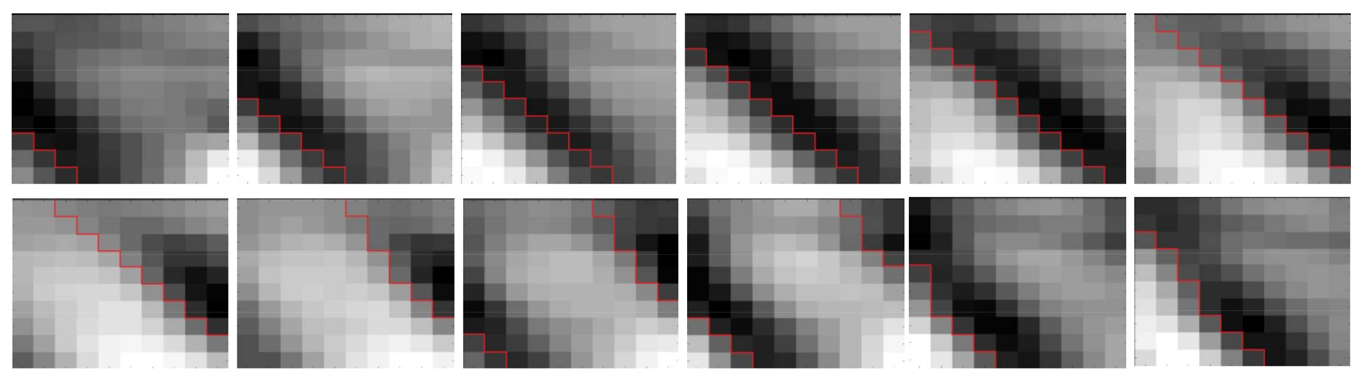
Figure 2.
The mode of wind speed prediction with spatio–temporal correlation.

Figure 3.
Structure of a typical convolutional neural network (CNN).

Figure 4.
The architecture of predictive deep convolutional neural network (PDCNN).

Figure 5.
Mutual information with τ from 0 to 20.

Figure 6.
The 10 × 10 wind turbine array in Indiana. Each wind turbine is marked as a black dot.

Figure 7.
The architecture of PDCNN.
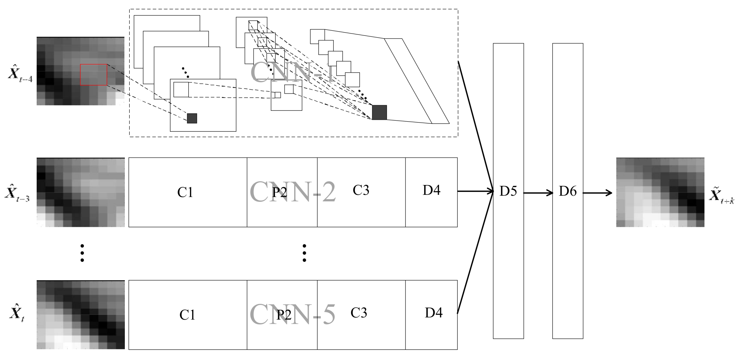
Figure 8.
Time complexity, with h ranging from 1 to 10 in the 5-min ahead prediction task.


Table 1.
Hyper-Parameters of Prediction Models.
| Prediction Horizon (Min) | PDCNN | MLP | SVR | DT | |
|---|---|---|---|---|---|
| a | b | C | γ | e | |
| 5 | 200 | 500 | 0.1 | 0.5 | 6 |
| 10 | 200 | 500 | 1.0 | 0.5 | 6 |
| 15 | 200 | 600 | 1.0 | 0.5 | 6 |
| 20 | 300 | 400 | 1.0 | 0.5 | 6 |
| 25 | 200 | 600 | 0.1 | 0.5 | 5 |
| 30 | 200 | 500 | 0.1 | 0.5 | 6 |
| 35 | 200 | 500 | 0.1 | 0.5 | 5 |
| 40 | 200 | 400 | 0.1 | 0.5 | 5 |
| 45 | 200 | 600 | 0.1 | 0.5 | 5 |
| 50 | 200 | 600 | 1.0 | 0.5 | 5 |
| 55 | 300 | 600 | 0.1 | 0.5 | 4 |
| 60 | 200 | 500 | 0.1 | 0.5 | 5 |
Table 2.
A-MAPE of Prediction Models for Different Time Horizons (%).
| Prediction Horizon (Min) | PR | MLP | SVR | DT | PDCNN |
|---|---|---|---|---|---|
| 5 | 7.179 | 6.665 | 6.901 | 6.740 | 4.414 |
| 10 | 8.246 | 7.091 | 7.455 | 7.194 | 5.463 |
| 15 | 9.153 | 7.756 | 7.343 | 7.402 | 5.526 |
| 20 | 9.804 | 8.046 | 7.746 | 8.070 | 6.299 |
| 25 | 11.058 | 9.085 | 8.535 | 8.395 | 6.703 |
| 30 | 12.197 | 9.619 | 9.371 | 9.105 | 6.992 |
| 35 | 13.259 | 10.311 | 9.990 | 10.008 | 7.252 |
| 40 | 14.236 | 10.663 | 10.790 | 11.471 | 7.622 |
| 45 | 15.105 | 11.240 | 11.670 | 11.498 | 8.183 |
| 50 | 15.905 | 11.597 | 12.608 | 12.799 | 8.912 |
| 55 | 16.677 | 12.418 | 13.378 | 13.028 | 8.948 |
| 60 | 17.431 | 13.170 | 14.223 | 14.018 | 9.306 |
Table 3.
A-RMSE of Prediction Models for Different Time Horizons (m/s).
| Prediction Horizon (Min) | PR | MLP | SVR | DT | PDCNN |
|---|---|---|---|---|---|
| 5 | 0.621 | 0.582 | 0.600 | 0.592 | 0.400 |
| 10 | 0.674 | 0.624 | 0.644 | 0.635 | 0.501 |
| 15 | 0.833 | 0.687 | 0.708 | 0.689 | 0.543 |
| 20 | 0.960 | 0.717 | 0.739 | 0.735 | 0.634 |
| 25 | 1.066 | 0.801 | 0.826 | 0.816 | 0.656 |
| 30 | 1.161 | 0.847 | 0.873 | 0.843 | 0.720 |
| 35 | 1.247 | 0.902 | 0.930 | 0.921 | 0.750 |
| 40 | 1.326 | 0.947 | 0.976 | 0.965 | 0.790 |
| 45 | 1.399 | 0.986 | 1.016 | 1.015 | 0.875 |
| 50 | 1.465 | 1.018 | 1.049 | 1.038 | 0.940 |
| 55 | 1.528 | 1.085 | 1.118 | 1.160 | 0.947 |
| 60 | 1.588 | 1.165 | 1.201 | 1.193 | 0.977 |
Table 4.
Maximum Instantaneous Error (MIE) of Prediction Models for Different Time Horizons (m/s).
| Prediction Horizon (Min) | PR | MLP | SVR | DT | PDCNN |
|---|---|---|---|---|---|
| 5 | 32.580 | 22.431 | 20.002 | 25.346 | 17.699 |
| 10 | 34.980 | 22.893 | 20.159 | 26.684 | 18.740 |
| 15 | 36.192 | 25.046 | 21.786 | 27.701 | 21.676 |
| 20 | 37.309 | 25.218 | 24.866 | 30.511 | 22.604 |
| 25 | 38.864 | 27.863 | 27.719 | 31.746 | 24.401 |
| 30 | 40.938 | 28.698 | 29.225 | 31.667 | 25.073 |
| 35 | 41.372 | 29.663 | 29.740 | 32.263 | 26.432 |
| 40 | 44.152 | 33.970 | 30.308 | 39.056 | 29.785 |
| 45 | 45.256 | 34.107 | 31.584 | 39.440 | 29.884 |
| 50 | 47.206 | 34.962 | 34.350 | 39.930 | 30.687 |
| 55 | 48.028 | 37.162 | 35.484 | 40.406 | 32.159 |
| 60 | 47.466 | 37.863 | 35.125 | 41.254 | 32.336 |
Table 5.
Prediction Performance for local MLPs (l-MLPs).
| Prediction Horizon (Min) | A-MAPE (%) | A-RMSE (m/s) | MIE (m/s) |
|---|---|---|---|
| 5 | 6.531 | 0.531 | 25.621 |
| 10 | 7.102 | 0.632 | 26.927 |
| 15 | 7.903 | 0.792 | 27.942 |
| 20 | 9.223 | 0.903 | 32.801 |
| 25 | 10.121 | 0.974 | 36.468 |
| 30 | 11.742 | 1.101 | 39.231 |
| 35 | 12.831 | 1.123 | 40.403 |
| 40 | 13.505 | 1.184 | 41.039 |
| 45 | 14.242 | 1.235 | 41.847 |
| 50 | 14.993 | 1.296 | 42.741 |
| 55 | 15.634 | 1.342 | 43.525 |
| 60 | 16.014 | 1.391 | 44.932 |
© 2018 by the authors. Licensee MDPI, Basel, Switzerland. This article is an open access article distributed under the terms and conditions of the Creative Commons Attribution (CC BY) license (http://creativecommons.org/licenses/by/4.0/).
Share and Cite
MDPI and ACS Style
Zhu, Q.; Chen, J.; Zhu, L.; Duan, X.; Liu, Y. Wind Speed Prediction with Spatio–Temporal Correlation: A Deep Learning Approach. Energies 2018, 11, 705. https://doi.org/10.3390/en11040705
AMA Style
Zhu Q, Chen J, Zhu L, Duan X, Liu Y. Wind Speed Prediction with Spatio–Temporal Correlation: A Deep Learning Approach. Energies. 2018; 11(4):705. https://doi.org/10.3390/en11040705
Chicago/Turabian StyleZhu, Qiaomu, Jinfu Chen, Lin Zhu, Xianzhong Duan, and Yilu Liu. 2018. "Wind Speed Prediction with Spatio–Temporal Correlation: A Deep Learning Approach" Energies 11, no. 4: 705. https://doi.org/10.3390/en11040705
Note that from the first issue of 2016, this journal uses article numbers instead of page numbers. See further details here.