Abstract
Actively controlling the camber angle to improve energy efficiency has recently gained interest due to the importance of reducing energy consumption and the driveline electrification trend that makes cost-efficient implementation of actuators possible. To analyse how much energy that can be saved with camber control, the effect of changing the camber angles on the forces and moments of the tyre under different driving conditions should be considered. In this paper, Magic Formula tyre models for combined slip and camber are used for simulation of energy analysis. The components of power loss during cornering are formulated and used to explain the influence that camber angles have on the power loss. For the studied driving paths and the assumed driver model, the simulation results show that active camber control can have considerable influence on power loss during cornering. Different combinations of camber angles are simulated, and a camber control algorithm is proposed and verified in simulation. The results show that the camber controller has very promising application prospects for energy-efficient cornering.
1. Introduction
As concern for environmental pollution and climate change grows, new energy-efficient vehicles, and in particular electric vehicles, have gained more and more attention. Electrified powertrains make decentralized driving systems possible, among which the in-wheel motors (IWM) are one important technology [1]. Electric vehicles with four in-wheel motors (4IWM) can directly and independently control their four wheels and can realise more advanced motion control than other types of vehicles. Besides better vehicle performance and safety control, energy-efficient control can also be carried out at the same time and has been considered a very important field of research, since energy-efficient electric vehicles can improve their popularity.
There are several studies about direct yaw moment control (DYC) for the improvement of vehicle handling and stability [2,3]. A 4IWM electric vehicle can easily implement DYC and the contribution of DYC to energy saving during cornering has been studied [4,5], but its contribution is normally limited. Other researchers are studying optimal torque distribution to improve energy efficiency [6,7], where the studies are usually conducted by incorporating the IWM efficiency map.
Electrification of vehicle actuators such as steering actuators and camber actuators provides opportunities for more advanced suspension designs, i.e., the active wheel corner module (ACM) [8], shown in Figure 1. In addition to 4IWMs, ACM can also realise individual wheel steering and active tyre camber control. In conventional vehicles, tyre camber angles are usually passively tilted according to suspension geometry that limits the possible ranges. Electric vehicles with ACM suspension design can have up to 12 control variables: 4 wheel drives, 4 steering controls and 4 camber controls. This is realised in the research concept vehicle with wheel corner module functionality, developed by KTH Royal Institute of Technology and shown in Figure 2 [9].
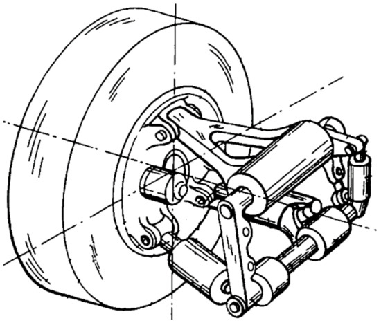
Figure 1.
Active wheel corner module [8].
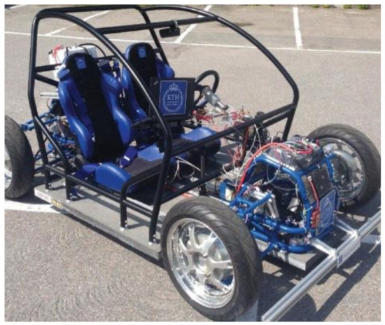
Figure 2.
KTH Research concept vehicle.
Camber angle is the angle between wheel plane and the normal to road [10]. For the simplicity of understanding camber control in this paper, the camber is defined as positive when the upper part of the tyre is lent to the left. Publications about controlling the camber angles to reduce energy consumption are quite few. There are some examples of research combining DYC with active camber control [11,12] and its effects on energy saving have also been studied [13,14]. From the results, the percentage of energy reduction seems promising. However, only camber’s effect on the lateral force was considered and no applicable camber controller has been suggested.
The aim of this work is to analyse how the camber affects power loss during cornering. The components of power loss, which includes the power to control camber angles are established. The longitudinal and lateral tyre forces interact with each other, especially in the case of high lateral acceleration during which the slip angle can be large enough to greatly influence the longitudinal forces. In addition, the camber angle could also cause changes to the forces and moments of the tyre [10,15,16]. For this reason, Magic Formula tyre models for longitudinal force, lateral force, overturning moment and aligning moment are adopted for simulation. Furthermore, a driver model and a method for camber control are designed to follow the designed paths. Two paths and three combinations of camber controls are chosen to primarily study camber’s effect on the components of power loss. After that, more comprehensive simulation settings are then studied and an applicable camber controller is proposed and verified by simulation.
2. Power Loss during Cornering
When a tyre travels with a camber angle, the component of rolling resistance moment on rolling resistance will be reduced and a component of aligning moment on rolling resistance will appear [17,18]. In this study, the kinetic equation describing the tyre taking into account the effects of camber angle is introduced. A two-track vehicle model is applied to derive the power loss during cornering, and the power needed to control the camber angles is estimated.
2.1. Tyre Kinetics with Camber Control
From Figure 3, the equation of motion in the longitudinal direction without camber control can be written as
where is the driving moment, is the rolling resistance moment, is the longitudinal force of the tyre, is the effective radius of the tyre, is the wheel rotational inertia and is wheel angular velocity.
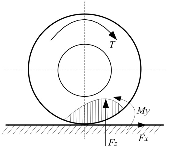
Figure 3.
Tyre without camber angle.
In Figure 4, the effect of camber is taken into account. X, Y and Z are coordinates of the road. Xw, Yw and Zw are coordinates of the tyre. While keeping the same camber angle during driving, the direction of is perpendicular to the wheel plane. The equation of motion can then be written as
where is the aligning moment and is the camber angle.
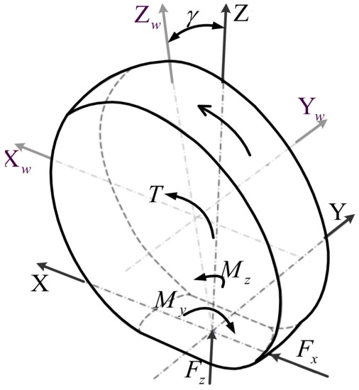
Figure 4.
Tyre with camber angle.
The rolling resistance moment can be expressed as
where is the vertical force of the tyre and is the rolling resistance coefficient.
2.2. The Power for Propulsion of the Wheels
As shown in Figure 5, a two-track vehicle model is formulated and front wheel steering is adopted. The longitudinal, lateral and yaw motions are formulated in Equations (4) to (6)
where, is the vehicle mass, is the longitudinal acceleration (), is the lateral acceleration (), is the forward speed, is the lateral speed, is the yaw angle, , , and are longitudinal forces at each tyre respectively, , , and are lateral forces at each wheel respectively, is the aerodynamic resistance, is the steering angles for the front wheels, is the moment of yaw inertia, is the distance from centre of gravity (CoG) to front axle, is the distance from CoG to rear axle, and is wheel track width (the subscript, 1: front left; 2: front right; 3: rear left; 4: rear right). The steering angle is assumed to be small (, ).
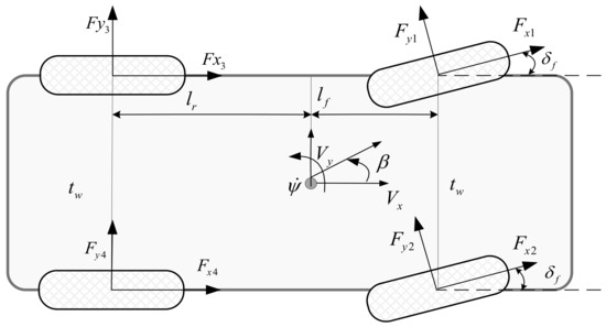
Figure 5.
Two-track vehicle model.
Slip angles (, , and ) for each wheel are expressed as
The angular velocity of the ith wheel can be expressed as
where is the slip ratio and is the forward speed of the ith wheel. The equations for forward speed for each individual wheel can be expressed as
The power for the propulsion of the wheels can be derived from the sum of the product of the driving moment and angular velocity of each wheel,
Re-writing Equation (2) for each wheel
By substituting Equations (4)–(9) as well as Equation (11) into Equation (10) makes it possible to reformulate as
where is aerodynamic loss, is rolling resistance loss, is longitudinal slip loss, is lateral slip loss, is longitudinal acceleration loss, is the wheel angular acceleration loss, is yaw acceleration loss, is lateral acceleration loss, and can be classified as additional loss.
For the aerodynamic resistance, can be expressed as:
where is the coefficient of aerodynamic resistance, is density of the air, and is frontal area of the vehicle. The vertical forces of each wheel are expressed as:
where is the height of CoG and is the acceleration of gravity (g = 9.8 m/s2).
2.3. The Power for Controlling Camber Angles
The power that is needed to control the camber angle for each tyre can be calculated by multiplying the overturning moment by the time derivative of the camber angle . It is not considered when . The estimated total power for controlling the camber angle of all four tyres is then,
The power loss during cornering is the sum of and i.e.,
3. Tyre Model
In this paper, Magic Formula tyre models for longitudinal force, lateral force, overturning moment and aligning moment under combined-slip and camber are used. Magic Formula is a semi-empirical equation that can closely match the experimental data [10]. The specific coefficients can be referred to in Appendix 3 of [10] and can be seen in Table 1, Table 2, Table 3 and Table 4.

Table 1.
Longitudinal force coefficients.
Table 2.
Lateral force coefficients.
Table 3.
Overturning moment coefficients.
Table 4.
Aligning moment coefficients.
3.1. Longitudinal Force
The equation of tyre longitudinal force under combined slip can be shown as
where
where , , , , , , , , , , , and are coefficients and is the nominal vertical force (). is weighting factor which is related to slip angle and camber angle of the tyre and can be expressed as
where , , , , and are coefficients and are shown in Table 1.
3.2. Lateral Force
The equation of tyre lateral force under combined slip can be shown as
where
where , , , , , , , , , , , , , , , , , , , , , , , , , , and are coefficients. is weighting factor which is related to slip ratio and camber angle of the tyre and can be expressed as
where , , , , , , and are coefficient and are shown in Table 2.
3.3. Overturning Moment
The equation of tyre overturning moment under combined slip can be shown as
where , , , , , , , , , and are coefficients and are shown in Table 3.
3.4. Aligning Moment
The equation of tyre aligning moment under combined slip can be shown as
where is the moment arm which arises for as a result of camber angle and lateral tyre deflection due to and can be expressed as
is the residual torque and can be expressed as
where
is pneumatic trail and can be expressed as
where
where , , , , , , , , , , , , , , , , , , , , , , , , , , , , , , and are coefficients and are shown in Table 4.
Examples of , , and under combined-slip conditions and camber are shown in Figure 6.
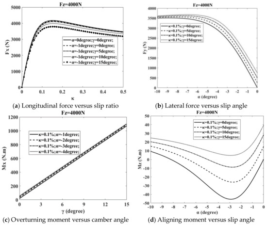
Figure 6.
Magic Formula tyre characteristics.
4. Energy Saving with Camber Control
In order to analyse how much contribution the camber can make to energy saving during cornering, paths are designed and a driver model is developed to follow the path and reference velocity. Then, a method for camber control is proposed and the changes in and the components in Equation (12) are analysed.
4.1. Path Design
By analysing the vehicle characteristics in steady-state cornering, the fundamental vehicle motion characteristics can be understood [19]. In steady-state cornering, the power remains constant. However, the dynamic power change during transient cornering when entering or exiting a corner is also important.
The chosen path is shown in Figure 7. The path consists of three parts: two straight lines with length L and a half-circle with radius R. In this paper, the longitudinal acceleration of the vehicle is not considered, namely, , i.e., the vehicle is assumed to follow the path at constant velocity. The vehicle first runs straight, then gradually reaches steady-state cornering (, and ) after entering the circle, after which it exits the circle and runs straight again.
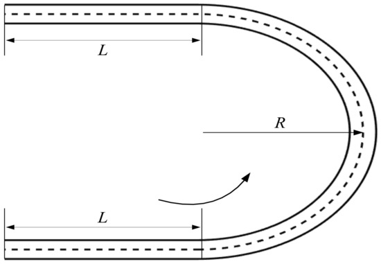
Figure 7.
Path design.
4.2. Driver Model
The driver model consists of two parts: a speed controller and a steering controller. In this paper, a PID speed controller is designed to follow the reference speed and the torques of the four wheels are assumed to be equal i.e., T1 = T2 = T3 = T4. The steering controller is based on the multiple-preview point steering theory [20,21,22]. Figure 8 shows a basic schematic diagram of this steering controller. As shown in the figure, the controller has three inputs: the lateral offset Δy1 between the vehicle and the road at the current position, the yaw angle offset Δψ between the vehicle yaw angle ψv and the road heading angle ψr and the lateral offset Δy2 at preview distance l ahead of the vehicle. The l is the product of preview time tp and the vehicle forward speed Vx, i.e., l = Vx tp. The front steering angle can be determined as
where , and are gains for each input.
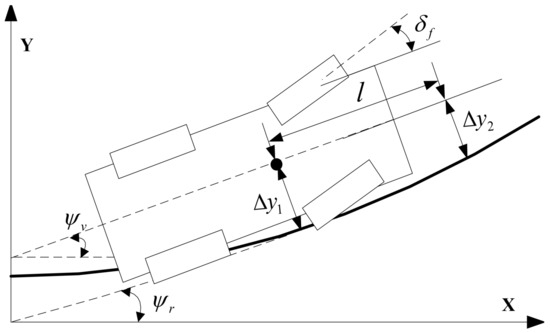
Figure 8.
Steering controller.
For the control of camber angle, the range of camber angle is assumed to be and for the path in Figure 7 the steering wheel is turned to the left and the range of the steering angle δf is . The camber angles of both front wheels, and , are set to the same value, and so are also the camber angles of both rear wheels, and , i.e., = and = . For the control of the camber angle, the relationships between camber angles and front steering angle are defined as:
where and are coefficients which determine the relationship between camber and steering angle. When or is larger than zero, this means that the front or rear wheels are tilted in the same direction as . Figure 9 gives rear views of the vehicle with camber control with different combinations of and .
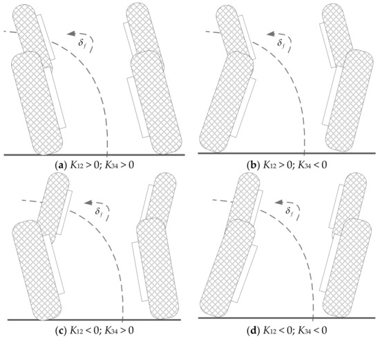
Figure 9.
Rear views of the vehicle with different settings on camber control coefficient K12 and K34.
4.3. Analysis of Components of Power Loss
In order to analyse how the power loss during cornering Pall changes, the simulation model is implemented in Matlab and Dymola. The simulation setups presented in Table 5 are used. The path parameters L = 60 m and R = 100 m are adopted; two lateral accelerations at steady-state cornering 3 m/s2 and 6 m/s2 are used and corresponding velocities are calculated; three different combinations of K12 and K34 are simulated. The Pall can be a function of K12 and K34 under a given path and velocity.
Table 5.
Parameters chosen for analysing the components of total power loss.
The vehicle parameters are shown in Table 6 and the density of the air is = 1 kg/m3. In [23], it was shown that the effect of camber on is low, so in this paper it is kept constant and is given a value of .
Table 6.
Vehicle parameters.
With the driver model, firstly the vehicle can keep the reference speed; secondly, the vehicle can track the reference path. Since the vehicle has the same speed and the same path with and without camber control, the simulation results can be compared. The aerodynamic loss remains the same at a certain velocity. At 62.3 km/h the aerodynamic loss is 1558 W and at 88.1 km/h 4406 W. The change in steering angle, camber angle, Pall, Pcamber, Pw and the components of Pw are shown in Figure 10 and Figure 11.
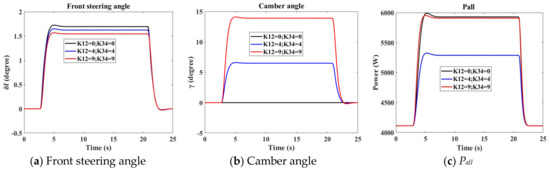
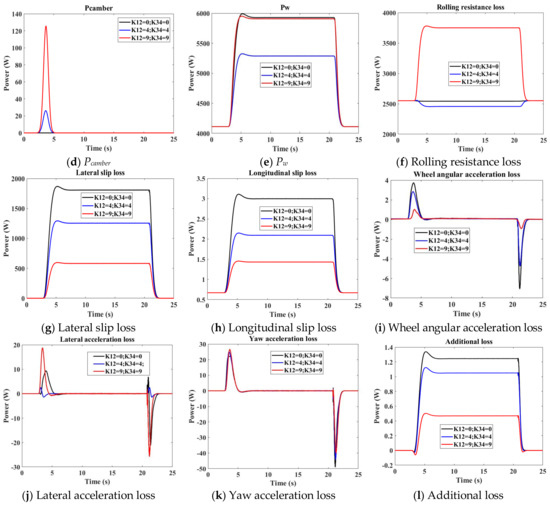
Figure 10.
Steering and camber angles as well as power losses at R = 100 m and Vx = 62.3 km/h.
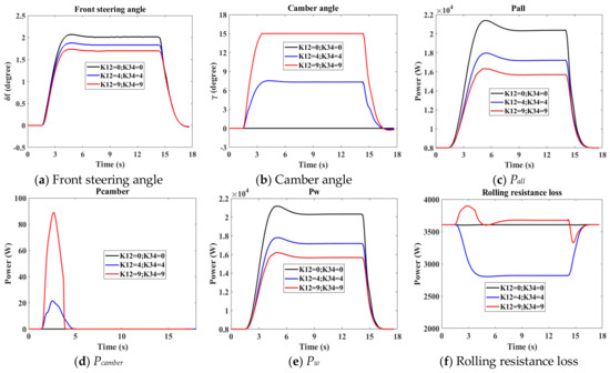
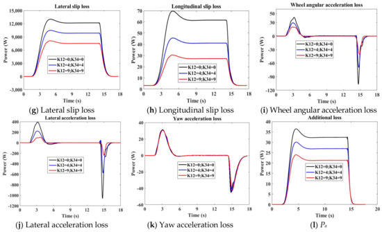
Figure 11.
Steering and camber angles as well as power losses at R = 100 m and Vx = 88.18 km/h.
If the same camber angles for front and rear tyres are implemented, the front steering angle does not change much from Figure 10a to Figure 11a. The main components of Pw are aerodynamic loss, rolling resistance loss and lateral slip loss. Although controlling camber can cost power, which is shown in Figure 10d and Figure 11d, the total power loss can still be reduced while entering the corner, which is shown in Figure 10c K12 = K34 = 4, 9 and Figure 11c K12 = K34 = 4, 9. From Figure 10g and Figure 11g, implementing positive camber control coefficients can greatly reduce lateral slip loss. The reduction of this part of power loss can be explained by studying Figure 6b. It is evident that keeping the same lateral force, the camber thrust can reduce the absolute value of slip angle and consequently, the lateral slip loss is reduced.
From Figure 6d, it is seen that camber angle can increase the aligning moment and this tyre property was also presented in [24]. The components of Mzi sinγi can have different influences on rolling resistance loss in different slip angle regions. From Figure 12, for R = 100 m, Vx = 62.3 km/h and ay = 3 m/s2, the slip angles are comparatively small. Compared to K12 = K34 = 4, the slip angles are further reduced by K12 = K34 = 9 and then all aligning moments become positive, which increases the rolling resistance substantially and greatly weakens the camber’s contribution to power reduction. However, from Figure 13, for R = 100 m, Vx = 88.18 km/h and ay = 6 m/s2, the slip angles are seen to be comparatively large. Consequently, further increasing the camber angle, does not increase much and the reduction of lateral slip loss still plays a dominant role in energy saving.
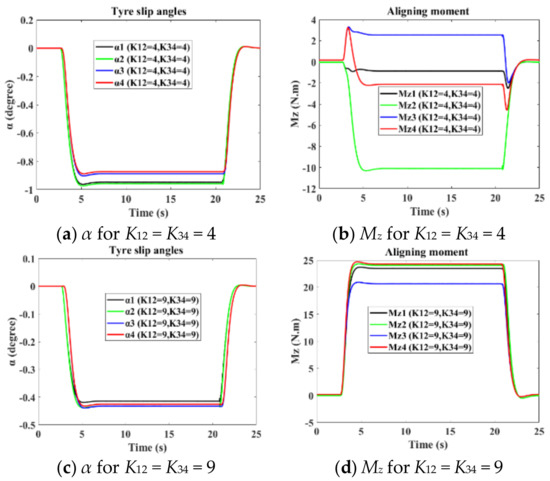
Figure 12.
Slip angle and aligning moment at R = 100 m and Vx = 62.3 km/h.
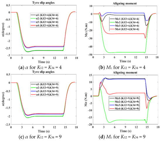
Figure 13.
Slip angle and aligning moment at R = 100 m and Vx = 88.18 km/h.
5. Controller Design for Camber
Compared to the power loss without camber , the percentage of energy saving with camber control can be described as
From Section 4, for R = 100 m, Vx = 62.3 km/h and ay = 3 m/s2, when , the camber angles at steady-state cornering are found to be 6.50 and is 8.31%; for R = 100 m, Vx = 88.18 km/h and ay = 6 m/s2, when , the camber angles at steady-state cornering are 150 and is 19.11%.
These results show that camber can be very promising to save energy during cornering. However, how to fully use the potential of camber for different driving scenarios remains to be explored and a camber controller needs to be designed. A more comprehensive test scheme has been developed and is shown in Table 7. Besides L = 60 m and R = 100 m, two groups of path parameters (L = 30 m, R = 50 m; L = 90 m, R = 150 m) are added. Six lateral accelerations (1, 2, 3, 4, 5 and 6 m/s2) at steady-state cornering are studied and corresponding velocities are deducted.
Table 7.
Path parameters, chosen velocities and lateral accelerations at steady-state.
Figure 14, Figure 15 and Figure 16 present the results for the simulation setups in Table 7 and the reference 0% energy saving planes are also plotted in these figures. Firstly, it is shown that the higher the lateral acceleration at steady-state cornering is, the more energy saving can be achieved. The main function of the camber control is to reduce the lateral slip loss and when the lateral acceleration is small during the cornering, the percentage of lateral slip loss of total power loss is small. Camber control therefore makes no significant contribution to energy saving. Because of different working slip regions of Mz introduced in Section 4.3, at low accelerations higher camber angle settings might increase rolling resistance loss considerably as can be seen from Figure 14a–c, Figure 15a–c and Figure 16a–c. For 6 m/s2, the results show that for larger values of K12 and K34, more energy can be saved. But for the rest of the lateral accelerations there are maximum energy saving points. Above all, these points are not singular and many combinations of K12 and K34 can be chosen for energy saving control.
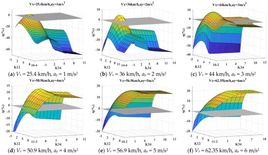
Figure 14.
Energy saving for different K12 and K34 for path R = 50 m and L = 30 m.
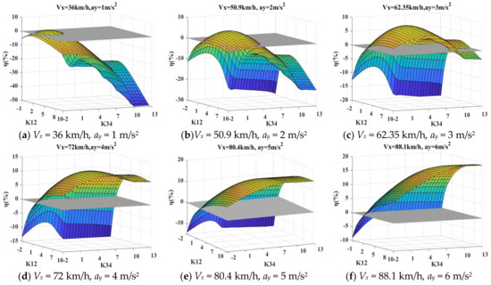
Figure 15.
Energy saving for different K12 and K34 for path R = 100 m and L = 60 m.
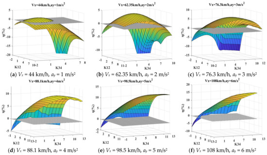
Figure 16.
Energy saving for different K12 and K34 for path R = 150 m and L = 90 m.
For the simplicity of the camber control, the same camber angles for the front and the rear tyres are preferred i.e., K12 = K34. To study these assumptions, the combinations of K12 and K34 are chosen and the camber angles during the steady-state cornering part are also shown in Table 8. These combinations are the optimal points or near the optimal ones. It can be seen that for certain ay during the steady-state cornering, the efficient camber angles are approximately equal.
Table 8.
The chosen combinations of K12 and K34 in the study.
As a consequence, it is assumed that the camber angle can be controlled with the information of ay. A controller which uses ay as criteria for the camber control is shown in Figure 17 and the mean value of the three camber angles in Table 8 for each lateral acceleration ay is used. Although, at high lateral accelerations such as 6m/s2 and above, camber setting larger than 15° may save more energy, the average driver generally drives below 4 m/s2 and 6 m/s2 or higher only occurs in extreme situations [25]. Also with the concern of suspension working space, 15° camber angle is still chosen for lateral acceleration higher than 6 m/s2 in this work.
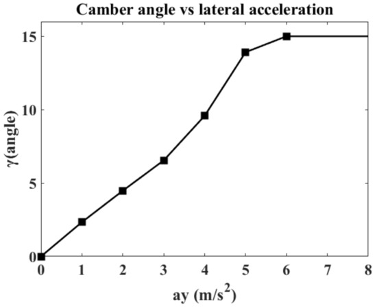
Figure 17.
Camber control versus lateral acceleration.
From Figure 10a and Figure 11a, although implementing camber control can reduce steering angle, the reduction is small and the linear relation between δf and ay for each constant velocity can be regarded to be unchanged. Therefore, a feedforward camber controller based on the information δf and Vx is designed for simulation purposes. With the designed camber controller, the percentages of energy saving for the chosen driving scenarios defined in Table 7 are shown in Figure 18. The results show that the designed camber controller has a very promising application prospect for energy saving.
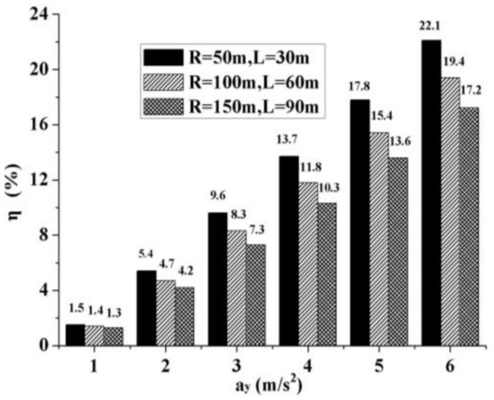
Figure 18.
Energy saving for camber controller.
6. Conclusions
In order to analyse how a variation in camber angles influences the power loss during cornering, this paper formulates the components of the power loss. Different paths and velocities are designed for evaluation of camber effects. In Section 4, three combinations of K12 and K34, two designed paths and two velocities are primarily studied. With camber control, the components of total power loss, which includes the power for controlling camber, are studied and from the results it is concluded that the three main components are aerodynamic loss, rolling resistance loss and lateral slip loss. For chosen combinations of K12 and K34, camber control can reduce lateral slip loss but can also cause different changes in rolling resistance loss. In Section 5, different combinations of K12 and K34, three paths and six velocities (corresponding to six accelerations at steady-state cornering) for each path are further studied.
The contribution of camber angle control to energy saving is obvious when lateral acceleration is high. There are multiple choices of K12 and K34 that can have a positive impact. The strategy of implementing the same camber angles for all tyres is chosen to be adopted. From Table 8, for each lateral acceleration the efficient camber angles are almost equal even if the velocities are different. The camber controller based on lateral acceleration is then developed and the effectiveness of the controller is evaluated. The results show that the proposed control algorithm is promising to save energy during cornering.
In future work, the longitudinal acceleration can be included and the tyre wear change due to camber control also needs to be considered. It is of great interest to explore expected energy saving within the probability density function of driving at various speeds and lateral accelerations with camber control. The change in the stability factors remains to be explored. Camber control is closely related to tyre properties and it is therefore important to know the tyre information before camber control is applied.
Acknowledgments
The authors greatly appreciate the financial support from China Scholarship council.
Author Contributions
Peikun Sun designed the simulation and wrote the paper. Annika Stensson Trigell, Lars Druggee, Jenny Jerrelind and Mats Jonasson contributed analysis methods.
Conflicts of Interest
The authors declare no conflict of interest.
References
- Murata, S. Innovation by in-wheel-motor drive unit. Veh. Syst. Dyn. 2012, 50, 807–830. [Google Scholar] [CrossRef]
- Wang, R.; Chen, Y.; Feng, D.; Huang, X.; Wang, J. Development and performance characterization of an electric ground vehicle with independently actuated in-wheel motors. J. Power Sour. 2011, 196, 3962–3971. [Google Scholar] [CrossRef]
- Xiong, L.; Yu, Z.; Wang, Y.; Yang, C.; Meng, Y. Vehicle dynamics control of four in-wheel motor drive electric vehicle using gain scheduling based on tyre cornering stiffness estimation. Veh. Syst. Dyn. 2012, 50, 831–846. [Google Scholar] [CrossRef]
- Kobayashi, T.; Katsuyama, E.; Sugiura, H.; Ono, E.; Yamamoto, M. Direct yaw moment control and power consumption of in-wheel motor vehicle in steady-state turning. Veh. Syst. Dyn. 2017, 55, 104–120. [Google Scholar] [CrossRef]
- Kobayashi, T.; Sugiura, H.; Ono, E.; Katsuyama, E.; Yamamoto, M. Efficient Direct Yaw Moment Control of in-Wheel Motor Vehicle. In Proceedings of the AVEC 13th International Symposium on Advanced Vehicle Control, Munich, Germany, 13–16 September 2016. [Google Scholar]
- Chen, Y.; Wang, J. Energy-Efficient Control Allocation with Applications on Planar Motion Control of Electric Ground Vehicles. In Proceedings of the ACC American Control Conference, Hilton San Francisco, CA, USA, 29 June–1 July 2011. [Google Scholar]
- Suzuki, Y.; Kano, Y.; Abe, M. A study on tyre force distribution controls for full drive-by-wire electric vehicle. Veh. Syst. Dyn. 2014, 52, 235–250. [Google Scholar] [CrossRef]
- Zetterström, S. Vehicle Wheel Suspension Arrangement. U.S. Patent 6,386,553, 14 May 2002. [Google Scholar]
- Wallmark, O.; Nybacka, M.; Malmquist, D. Design and Implementation of an Experimental Research and Concept Demonstration Vehicle. In Proceedings of the IEEE VPPC Vehicle Power and Propulsion Conference, Coimbra, Portugal, 27–30 October 2014. [Google Scholar]
- Pacejka, H. Tyre and Vehicle Dynamics; Elsevier: Amsterdam, The Netherlands, 2012. [Google Scholar]
- Manipal, K. Control of Vehicle Yaw Moment by Varying the Dynamic Camber. In Proceedings of the 11th International Symposium on Advanced Vehicle Control, Seoul, Korea, 9–12 September 2012. [Google Scholar]
- Yutaka, H. Integrated Control of Tire Steering Angle, Camber Angle and Driving/Braking Torque for Individual in-Wheel Motor Vehicle. In Proceedings of the 11th International Symposium on Advanced Vehicle Control, Seoul, Korea, 9–12 September 2012. [Google Scholar]
- Jerrelind, J.; Edrén, J.; Li, S. Exploring Active Camber to Enhance Vehicle Performance and Safety. In Proceedings of the 23rd International Symposium on Dynamics of Vehicles on Roads and Tracks, Qingdao, China, 19–23 August 2013. [Google Scholar]
- Davari, M.M.; Jonasson, M.; Jerrelind, J. Rolling Loss Analysis of Combined Camber and Slip Angle Control. In Proceedings of the AVEC’16, 13th Symposium on Advanced Vehicle Control, Munich, Germany, 13–16 September 2016. [Google Scholar]
- Svendenius, J.; Gäfvert, M. A Brush-Model Based Semi-Empirical Tire-Model for Combined Slips. SAE Technical Paper. 2004. Available online: https://www.sae.org/publications/technical-papers/content/2004-01-1064/ (accessed on 21 March 2018).
- Svendenius, J.; Gäfvert, M.; Bruzelius, F.; Hultén, J. Experimental validation of the brush tire model. Tire Sci. Technol. 2009, 37, 122–137. [Google Scholar] [CrossRef]
- Genta, G. Motor Vehicle Dynamics: Modeling and Simulation; World Scientific: Singapore, 1997. [Google Scholar]
- Jazar, R.N. Vehicle Dynamics: Theory and Application; Springer Science & Business Media: Berlin/Heidelberg, Germany, 2013. [Google Scholar]
- Abe, M. Vehicle Handling Dynamics: Theory and Application; Butterworth-Heinemann: Oxford, UK, 2015. [Google Scholar]
- Sharp, R.S.; Casanova, D.; Symonds, P. A mathematical model for driver steering control, with design, tuning and performance results. Veh. Syst. Dyn. 2000, 33, 289–326. [Google Scholar]
- Winkler, N.; Drugge, L.; Trigell, A.S. Coupling aerodynamics to vehicle dynamics in transient crosswinds including a driver model. Comput. Fluids 2016, 138, 26–34. [Google Scholar] [CrossRef]
- Wanner, D.; Drugge, L.; Edrén, J.; Trigell, A.S. Modelling and Experimental Evaluation of Driver Behaviour during Single Wheel Hub Motor Failures. In Proceedings of the FASTzero’15 International Symposium on Future Active Safety Technology Towards Zero Traffic Accidents, Gothenburg, Sweden, 9–11 September 2015. [Google Scholar]
- Davari, M.M.; Jerrelind, J.; Trigell, A.S. Extended brush tyre model to study rolling loss in vehicle dynamics simulations. Int. J. Veh. Des. 2017, 73, 255–280. [Google Scholar] [CrossRef]
- Fujioka, T.; Goda, K. Tyre cornering properties at large camber angles: mechanism of the moment around the vertical axis. JSAE Rev. 1995, 16, 257–261. [Google Scholar] [CrossRef]
- Bosch, R. Automotive Handbook; Robert Bosch GmbH: Gerlingen, Germany, 2011. [Google Scholar]
© 2018 by the authors. Licensee MDPI, Basel, Switzerland. This article is an open access article distributed under the terms and conditions of the Creative Commons Attribution (CC BY) license (http://creativecommons.org/licenses/by/4.0/).