Identification and Evaluation of Cases for Excess Heat Utilisation Using GIS
by
 , , ,
, , ,
Fabian Bühler
1,* ,
,
Stefan Petrović
2,
Torben Ommen
1,
Fridolin Müller Holm
3,
Henrik Pieper
1 and
Brian Elmegaard
1 1
Department of Mechanical Engineering, Technical University of Denmark, 2800 Kongens Lyngby, Denmark
2
Department of Management Engineering, Technical University of Denmark, 2800 Kongens Lyngby, Denmark
3
Viegand Maagøe A/S, 1364 København, Denmark
*
Author to whom correspondence should be addressed.
Energies 2018, 11(4), 762; https://doi.org/10.3390/en11040762
Submission received: 1 March 2018
/
Revised: 21 March 2018
/
Accepted: 22 March 2018
/
Published: 27 March 2018
(This article belongs to the Special Issue Industrial Energy Efficiency 2018)
Abstract
:Excess heat is present in many sectors, and its utilization could reduce the primary energy use and emission of greenhouse gases. This work presents a geographical mapping of excess heat, in which excess heat from the industry and utility sector was distributed to specific geographical locations in Denmark. Based on this mapping, a systematic approach for identifying cases for the utilization of excess heat is proposed, considering the production of district heat and process heat, as well as power generation. The technical and economic feasibility of this approach was evaluated for six cases. Special focus was placed on the challenges for the connection of excess heat sources to heat users. To account for uncertainties in the model input, different methods were applied to determine the uncertainty of the results and the most important model parameters. The results show how the spatial mapping of excess heat sources can be used to identify their utilization potentials. The identified case studies show that it can be economically feasible to connect the heat sources to the public energy network or to use the heat to generate electricity. The uncertainty analysis suggests that the results are indicative and are particularly useful for a fast evaluation, comparison and prioritization of possible matches. The excess heat temperature and obtainable energy price were identified as the most important input parameters.
Keywords:
heat recovery; industry; utility; district heating; power generation; excess heat; energy efficiency1. Introduction
Excess heat is available from many sources, and its avoidance or utilization would reduce the primary energy use and greenhouse gas (GHG) emissions associated with the burning of fossil fuels. The full recovery of excess heat is connected to several challenges and barriers. Even if cost-effective measures are available, they are often not implemented. This is often referred to as the ‘energy efficiency gap’ [1]. Several studies [2,3,4] analyzed possible barriers specific to industrial excess heat utilization. The lack of available information and knowledge about excess heat and potential excess heat users was found to be a major barrier in all three studies. Structural barriers, such as the lack of infrastructure for heat transmission and a limited technical recovery potential, were identified as additional barriers. Economic barriers also play an important role, such as the initial costs of obtaining information and missing governmental frameworks.
To overcome some of these challenges and barriers, a fast and comprehensive method for identifying utilization potentials of excess heat and evaluating their technical and economic feasibility is required. The method presented in this work contributes to solving some of these issues. It allows energy planners, district heating operators and industrial plant managers to find synergies between emitters of excess heat and heat demands on a local level and quickly assess specific cases, before performing detailed analyses.
Research has so far focused on the quantifying of excess heat and the temperature levels, as well as analyzing potentials for utilization. A number of studies quantified the amount of industrial excess heat, such as Miró et al. [5] for waste heat in different countries and regions and Naegler et al. [6] on a European level. Brückner et al. [7] reviewed the methods developed to estimate the waste heat potential of regions. The reviewed methods and literature in this study were categorized into two categories, namely surveys and estimates. The classification did not specifically take the geographical locations of the heat sources into account. However, size parameters for companies, such as the number of employees, were used to classify the estimations of the excess heat. Miró et al. [8] showed how CO emission data can be used to find industrial waste heat recovery potentials. The method was based on McKenna and Norman [9], who presented a spatial model of industrial heat loads and technical recovery potentials in the U.K. Persson et al. [10] applied a similar approach to identify heat synergy regions in Europe, also solely relying on CO emission data.
Brückner et al. [11] investigated the utilization of waste heat for residential heating in an urban neighborhood in Germany and performed an economic analysis of heat transformation technologies for industrial waste heat [12]. For Sweden, Broberg et al. [13] estimated the potential of industrial excess heat for Swedish district heating networks and showed, based on cost calculations, how excess heat investments become profitable. Viklund and Johansson [14] further reviewed the technologies for the utilization of excess heat and estimated their potential for a region in Sweden. Eriksson et al. [15] analyzed the economic performance of exporting industrial excess heat from a chemical complex site in Sweden. A heat sale price of 200 SEK per MWh was found most probable. The uncertainties and complexity of the local heat market made an investment focused on delivering district heat the more risky option compared to recovering heat on site. Karner et al. [16] modeled synergies of industrial sites with urban areas, considering amongst others the use of industrial heat for urban heating. The results showed that for heat-related investments, there was profitability even without investment funding and that there was a high difference between heat pump and direct utilization cases. Li et al. [17] analyzed and optimized different configurations for a district heating network based on a distant low-temperature industrial excess heat source. For the case of Northern China, the authors found that even if the heat source was distant, the economic and environmental advantages justified the excess heat utilization.
An analysis by Hammond and Norman [18] showed the heat recovery opportunities in the U.K.’s industry for 11 industrial sectors. The utilization potential for different technologies was found considering the waste heat temperature. An analysis of heat transportation between sites with surplus heat and heating demand was further performed. Another study for the U.K. [19] investigated the potential of using industrial excess heat for district heating. Approximately one third of the U.K. excess heat was found to be potentially usable for district heating when the only constraint was a limited transmission distance. A study performed by Lund and Persson [20] analyzed the Danish potential of low-temperature heat sources for use in district heating networks by heat pumping. Besides low-temperature industrial excess heat and supermarket refrigerators, their work considered natural sources such as ground water and lakes. Based on this analysis, a theoretical potential for the utilization of low-temperature heat in Denmark can be identified. The work of [21,22] also used Denmark as a case study and analyzed in detail the utilization potential of industrial excess heat for district heating, taking into account spatial and temporal constraints. Furthermore, the heating prices for industrial excess heat were determined, indicating that a majority of the excess heat can be used for district heating at competitive socio-economic costs. An analysis and evaluation of four case studies for the excess heat utilization using GIS and techno-economic calculations were presented by Bühler et al. [23]. The current work originated in the applied methods and case studies of the previous study. The GIS model data were used for more case studies; the model and assumptions were improved; and the uncertainty and sensitivity analysis were extended.
This article provides a method to overcome some of the barriers to excess heat utilization and extends the current state of research by spatial and economic analyses of excess heat sources and possible users, including uncertainty and sensitivity analyses. This method builds on the application of geographical information system (GIS)-based data to excess heat and heating demand to identify and evaluate the feasibility of relevant cases for the utilization of excess heat. The evaluation of the feasibility was based on technical practicability, as well as economic indicators for each case. By using uncertainty and sensitivity analyses, the validity and confidence intervals of the method were analyzed.
The approach and method for identifying potential synergy cases and the background of the data are first described in detail. Based on exemplarily identified excess heat cases with GIS, six were selected and further analyzed. This analysis included: (i) technical considerations, such as the annual profiles and operating hours of heat sources and sinks, the available and required temperature levels; (ii) economic considerations for the investment in new equipment, its operation and maintenance; (iii) governmental frameworks (in particular taxes and subsidies); and (iv) environmental considerations, such as the type of replaced heating fuel and avoided GHG emissions. Eventually, an uncertainty analysis of the models was conducted to determine the confidence of the result, and a sensitivity analysis was performed to determine the most important input parameters to allow an optimized application of the model.
2. Methods
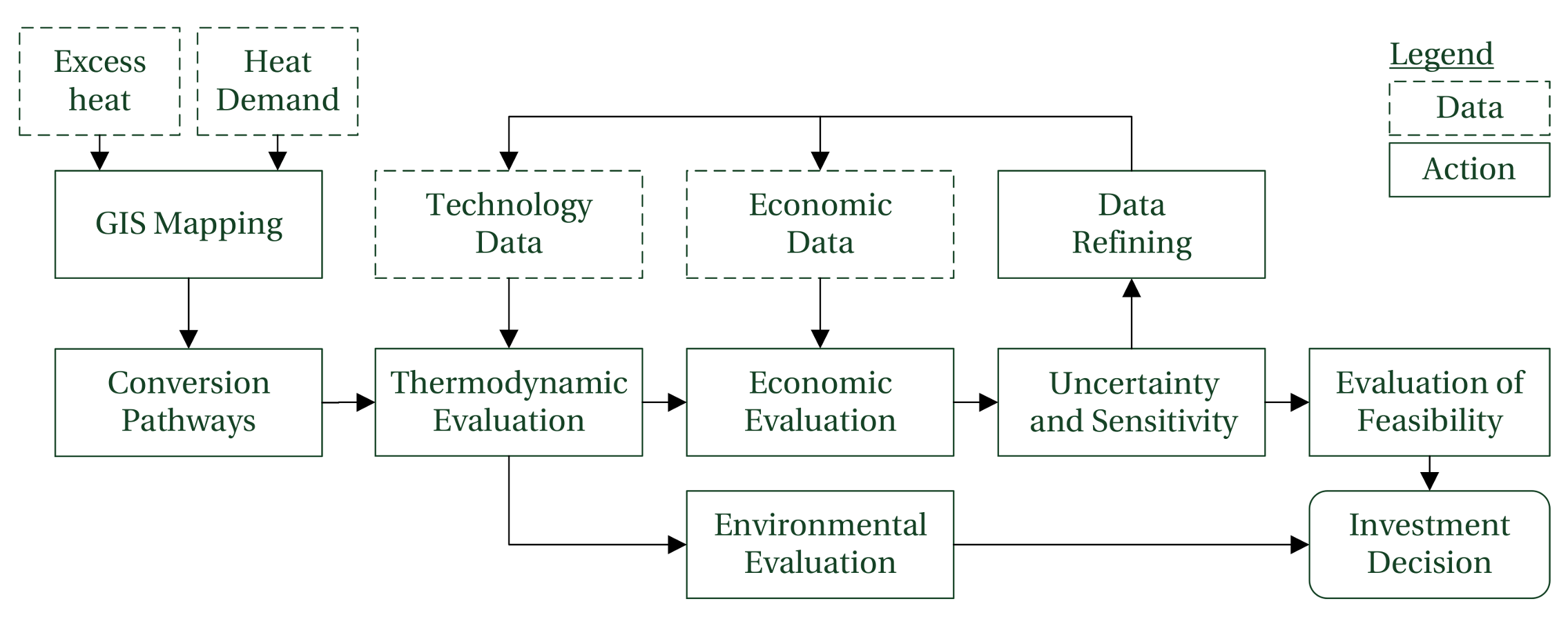
In the following, the method for evaluating the feasibility of excess heat (EH) utilization for the supply of different energy demands is shown. The overall method and setup of the tool is shown in Figure 1. Based on data for the excess heat and heat demand, a GIS mapping was performed, which was used to identify opportunities to recover EH. Based on the identified case, first a thermodynamic evaluation followed by an economic one was performed. For the model outcomes of these two evaluations, an uncertainty and sensitivity analysis was conducted. This allowed a targeted refinement of the key parameters, to increase the confidence in the model output. At the end, the results of the economic evaluation, including the uncertainties, together with an environmental assessment were used to evaluate the overall feasibility of the cases and make the investment decision. These results can then be used to make the decision if further investigations by, e.g., consultants should be made.
2.1. Geographical Mapping and Identification of Synergies
This work originates from earlier studies where industrial excess heat from thermal processes and its temperature levels were determined for production sites in Denmark [21,22,24]. The excess heat was found by distributing the energy use in Denmark [25] to the thermal processes of 22 industrial sectors [26] and determining for each the excess heat amount and temperature level. Based on the aggregated numbers, a spatial distribution of excess heat to production sites was performed. This distribution took, depending on the availability of data, the energy use, CO emissions and number of employees at the production sites into account. As this method relied on a top-down approach, using statistical data, the final numbers were connected with uncertainties, which should be considered when using them. The method for case identifications itself was presented in [23] and showed the potential of using industrial excess heat for district heating in Denmark. In the current analysis, an identical distribution key was used to include other industrial excess heat sources, as they were found in [27]. This excess heat mapping took into account all processes and the energy use of all industrial sectors and the utility sector. The level of detail was however lower, as process-specific excess heat mappings were performed, which were applied to the whole sector. Excess heat from the utility sector (power and heating plants) and waste water treatment (WWT) plants was further included in this work. The aggregated EH data were distributed to specific locations using the individuals plants’ thermal or electric capacity [28] and the amount of treated waste water [29]. District heating areas [30] and their respective heating demands, fuel use and heating costs [31] were further integrated in the GIS model. All the above data were integrated and analyzed using QGIS [32], an open source GIS software, with map material from OpenStreetMap (OSM) [33].
In this analysis, the utilization of excess heat for heating of buildings or industrial processes, as well as the generation of electricity was considered. To identify specific cases where the use of excess heat could be feasible, the detailed evaluation of the technical and economic feasibility of these cases was performed as follows:
- Evaluation of the maximum amount of industrial EH, which can be converted to district heat substitution, as performed in [21].
- Identification of district heating areas with high substitution potential; analysis of the excess heat sources responsible for the high potential in GIS.
- Assessment of the EH sources: sector of the match and company, typical excess heat amount and temperatures for processes of the sector and determination of the distance to the nearest heating area; for each heat sink, the most suited heat source was considered.
- Economic and technical evaluation of the case: this requires the estimation of typical operating hours and profiles, as well as the determination of current heating prices, investment and operating costs.
In case a synergy between two industrial complexes was found, the replacement of process heat with excess heat was considered in a similar manner. Instead of the second step, clusters of excess heat were identified. Such clusters can indicate the presence of many companies from the industry and utility sector. Using the excess and process heat temperatures of individual sites, matches between them could be found.
The evaluation of cases for electricity production were found by identifying industrial sites that either have (i) high-temperature excess heat (>150 C) from other sources than off-gases from boilers or (ii) are in isolated locations.
In Section 2.2 and Section 2.4, the technical and economic evaluation of the matches are described and performed. The aim was to obtain an indication of the feasibility, which justifies further analyses. The feasibility evaluation was performed, which required the following characteristics: the temperature of the EH, the amount of EH, the classification of the industrial sector, as well as the temperatures, capacity and type of heat sinks. This information was included for each site in the GIS model on a sectoral level. Further refining of the data was required for the individual processes by using information from the literature.
2.2. Utilization of Excess Heat
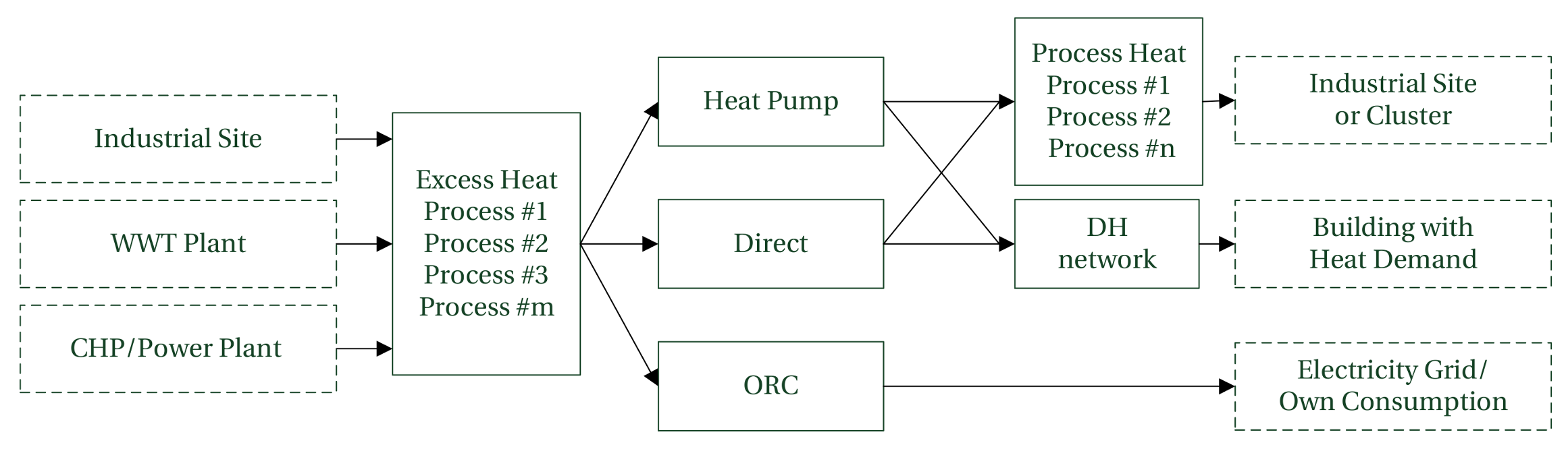
The utilization pathways for the use of excess heat, considered in this work, are shown in Figure 2. Three technologies were considered, namely direct heat transfer, heat pumping and organic Rankine cycles (ORC). The considered uses of the excess heat were: industrial sites requiring process heat, heat demand of buildings and the electrical grid.
The direct utilization of the excess heat was possible when the source temperature, , was by the minimum temperature difference , higher than the required supply temperature, , of the heat sink. It was assumed that the excess heat was transferred to the district heating network via one heat exchanger. If the excess heat was delivered to another process heat, a heat transfer loop between the two sites was considered a requirement. Such a heat transfer loop requires a second heat exchanger on the sink site.
A heat pump was required when the temperature of the excess heat , after the subtraction of the minimum temperature , was below the required supply temperature. The works by Jensen et al. [34] and Ommen et al. [35] showed that some part of the heat could be transferred directly. In this work, it was assumed that all the heat passed the heat pump. The heat pump was modeled using the Lorenz cycle and was corrected by the Lorenz efficiency to obtain the real coefficient of performance (COP), as shown in Equation (1). For the logarithmic mean temperature of the heat source and heat sink, Equations (2) and (3) were used.
The third option was to use an ORC to generate power from the excess heat in cases where no suitable heat sink was present or if the temperature of the excess heat was high and power generation was seen as the favorable option. In those cases, the electrical efficiency of the ORC mainly depended on the excess heat temperature. In this work, the efficiency of the ORC was found using Equation (4). The theoretical efficiency of converting heat to power is described by the Carnot efficiency . To obtain a more realistic result, the Carnot efficiency is multiplied with an electrical efficiency, , which is between 30% and 50% for EH sources in a temperature range of 100 C–350 C. The choice of the electrical efficiency was based on literature correlations [14,18,36], and was set to the environmental state at 25 C. The option of utilizing the heat from the condenser of the ORC was not particularly considered in this work, but it could be relevant in some cases.
The minimum temperature difference considered in this work was 5 K for streams below 60 C, which were assumed to be liquid and originating from, e.g., condensate or compressor cooling. For streams above 60 C, a value of 10 K was used, accounting for the mainly high-temperature exhaust gas flows. It was further chosen to set a minimum outlet temperature for EH streams to 40 C if they were above 60 C and to 15 C if they were below. Only for waste water, a constant temperature difference of to of 6 K was chosen [37]. If the DH return temperature was above the minimum outlet temperature, the return temperature was used.
To determine the investment costs, the heating capacity of the heat pump and the electric power for the ORC were used. In the case of a direct heat transfer, the area of the heat exchanger was found using Equation (5), where LMTD is the logarithmic mean of the temperature difference in counter-current heat exchanger and k the fixed overall heat transfer coefficient.
2.3. Excess Heat and Heating Demand
The excess heat source, as well as the heating demand are often varying over time. These variations made it necessary to account for their operating profile in relation to each other. In this work, seasonal profiles were used to correct the possible utilization of excess heat towards different source and sink profiles. The profiles allocate the heat demand and supply over four quarters of the year (Q1–Q4) as shown in Table 1. Q1 represents the heat demand in the three first months of the year, Q2 the following three months, and so forth. Two profiles were created for heat demands (DH1 and DH2), and four profiles were considered for the industrial plants (P1 to P4). The industry profiles take into account that some industries have a constant production (e.g., chemical and food industry) and some have a higher production during warm periods or vice versa (e.g., building materials). The first heat demand profile, DH1, follows the annual residential heating demand. To account for situations where the summer heat demands in a DH area are covered by waste incineration plants or solar heating, and thus no additional heat is needed, the DH2 profile was created.
Another factor that was critical for the determination of the particular sizes of equipment, as well as economic feasibility was the annual operating hours of a source or sink. If the excess heat is emitted in relatively small periods of time, the maximum power will be higher and require larger components. To account for variations of the operating hours, a selection was made based on the number of working shifts at the site. The typical operation profiles allow for three shifts, which was translated into 3200, 5000 or 8000 operating hours a year. There are also daily variations of the sink and source; however, it was assumed that these variations can be neglected as storage tanks of reasonable sizes could be implemented and act as buffers between supply and demand.
2.4. Economic Evaluation
The economic evaluation of each case study was performed by determining the economic feasibility, based on the investment (I) and the operation and maintenance (O&M) costs. The framework for investment was accounted through inflation, interest rates and future change in energy prices. Investment and operating costs are presented in Section 2.4.1. A separate focus of the economic analysis was the inclusion of taxes and subsidies in Denmark and how they influence the feasibility of the projects. An elaboration of this aspect is further presented in Section 2.4.2.
2.4.1. Investment and Operating Costs
The considered investment costs for utilizing the excess heat in this work consisted of the piping between heat source and sink, heat exchangers and heat pumps, as well as investments in equipment for an ORC if electricity was to be produced. Investment and maintenance costs were found amongst others using the Danish Technology Catalogue [38] and for piping the summary by Nielsen and Müller [39]. The equipment lifetime of 20 years for the economic analysis was chosen to be equal in all cases and for all equipment. Some equipment, i.e., DH pipes, will have a longer investment horizon than others, e.g., heat pumps. The found investment costs were seen as direct costs (DC), to which indirect costs as a fraction of the DC were added [40]. The investment costs were then obtained by deducting investment subsidies and adding interest payments on loans.
District heating prices were found for each heating area in the price statistics of the Danish Energy Regulatory Authority [41], which were used to correct the overall substitution given in Table 2. Future increases in DH prices depend on the specific DH area, in particular if it is a central or decentral area and the size. The Energy Producers Count [28] groups district heating producers into central and decentral, which supply the respective areas. Central DH areas have higher heat demands, installed capacities and transmission efficiencies compared to decentral DH areas. Different predictions were found, but a uniform prediction over all areas was chosen in this work [42]. It was further assumed that no costs were initially allocated to the excess heat and that the investment was performed by the owner of the excess heat source.
2.4.2. Taxes and Subsidies
In this work, the applicable taxes on EH utilization and electricity for EH recovery were considered, which depend on the excess heat sources and utilization technologies. For each of the considered pathways in the model, a brief overview is given for the Danish legislation based on [47,48]. Companies in Denmark are generally obliged to pay a tax on the utilized excess heat when the heat originates from a process and is used by a special installation for a non-process purpose. The tax on surplus heat can be based on the legislation, regulating the taxation of energy for process and non-process purposes. The aim of the surplus heat tax is to make sure that no speculation is made to avoid paying an energy tax for similar energy uses. The tax on surplus heat is put in place to compensate for a missing tax payment when process excess heat subsequently is used for a higher tax category as, e.g., space heating.
With respect to the chosen cases in this work, the excess heat sources are process heat, utility systems and waste water. These sources may be utilized for space heating, hot water, process heating and electricity generation. Furthermore, only the case of external utilization was considered, excluding the possibility of process integration, meaning recovering the excess heat for use within the factory. The following taxes and subsidies were considered:
- (i)
- Process heat for district heating (directly or via heat pump): If the excess heat is sold to a district heating company without using a heat pump, the payable tax is the difference of the space heating tax (6.75 € MWh) and the process heat tax. The tax is however capped to be no higher than 33% of the excess heat price paid by the district heating company. Furthermore, a tax reduction is obtainable when a heat pump is used. The taxable heat is then reduced to the difference of the excess heat and twice the electricity needed, meaning only the heat produced at the COP above three is taxed.
- (ii)
- Electricity generated from excess heat: The electricity generated from excess heat has no energy tax, as it currently is for all fuels. There are environmental taxes (e.g., NOx and SOx) for burning of fuels though, which are not relevant in this work. Taxes only occur for the use of electricity, and if the electricity is generated using renewable sources, tax credits of up to 20 € MWh can be applicable.
- (iii)
- Electricity tax for heat pumps using excess heat: A tax has to be paid on electricity used for space heating, which also applies to electricity used in the heat pump. This adds the public service obligation (PSO), electricity tax for space heating and the fee for the transmission system operator (TSO) to the net electricity price. In the future, these taxes will change. The Danish government decided to reduce the electricity tax for space heating gradually between 2019 and 2021 [49]. Furthermore, the the PSO will be phased out until 2022 [42].
- (iv)
- Subsidies for excess heat utilization: The sale of energy savings to utility companies was included in the form of an investment subsidy. This subsidy is based on the obligation imposed on utility companies by the government to save each year a certain amount of energy [50]. Industries, for example, have the possibility to sell their energy saving projects to utility companies, to help them achieve their targets. Based on average market prices in the year 2016, the value of one MWh saved of energy was chosen to be 54 €. This price depends however on the supply and demand, the utility company it is sold to and at which time of the year the energy savings are offered on the market. This results in an uncertainty, which was estimated to be ±15% of the base value.
2.4.3. Economic Evaluation and Comparison
The economic evaluation was performed by first calculating the unit costs of the heat supplied or electricity produced over the lifetime compared with the local energy prices. This included the investment costs I, the annual fixed and variable operation and maintenance (O&M) costs, and , the annuities, eventual subsidies and the costs of energy (heat or electricity) recovered from the excess heat.
Investment costs were found for each case study and included the DH pipes, heat exchangers, heat pumps, ORC and thermal energy storages, if applicable. For the operation of the system, the electricity prices for heat pumps were used, together with maintenance costs for HP, ORC and heat exchangers as described in the following section. The unit costs of heat, , were found with Equation (6) as the sum of annuity of the investment costs and O&M costs over the lifetime divided by the annual DH production, . The capital recovery factor (CRF), used to annualize the investment costs over the economic lifetime, , was found using the interest rate, i, as shown in Equation (7).
At the end, the private-economic investment calculation was performed from the viewpoint of the owner of the EH source. Here, the revenue for the sold heat was set at 85% of the the difference between average price in the specific DH area and the heating price of the EH source. The share of the revenue depends on negotiations between the excess heat owner and heat consumer. In general, it was assumed that the investor of the equipment takes the higher risk and therefore receives a higher share of the revenues. For electricity generation, the net electricity price was used. Based on this, the net present value (NPV) was found using Equation (8), where d denotes the discount rate and the cash flow in year n. In addition to the NPV, the internal rate of return (IRR) was found by solving Equation (8) for the discount rate with an NPV of zero.
2.5. Uncertainty and Sensitivity Analysis
To quantify the uncertainty of the model output, the Monte Carlo (MC) method was used [51]. With this method, the probability of the model output was determined, considering the uncertainty of inputs. With the MC method, the model was evaluated several times, using random input values generated within the input uncertainty space. The sampling of the input space was performed with Latin hypercube sampling (LHS). LHS is an efficient and proven method, able to produce more stable results than for instance random sampling [52]. The approach of this analysis was based on the work by Sin and Gernaey [53]. The quantification and representation of the input uncertainty is shown in Table 2, Table 3 and Table 4. In addition to these values, the available excess heat and operating hours were described with an uncertainty of ±20% with uniform distribution. The excess heat temperatures were varied within ±20 K and the ones of waste water with ±4 K. Four types of uncertainty distribution were chosen to optimally describe the input parameters, namely normal (N), half-normal (HN), uniform (U) and gamma (g). In this work, the mean and standard deviation are reported for the results. The model was simulated using 1500 samples, which yielded stable results. A more detailed analysis was made to take into account the dispersion of the model output, by graphically representing the data in box plots.
In order to identify the most important model input parameters, Morris screening [58] and linear regression of the MC simulations were used in this work for the sensitivity analysis. The Morris screening estimates the elementary effects (EE) for all uncertain input parameters on the model output. First, samples were created using the Morris sampling strategy, followed by evaluating the model with the created samples. The EE were then determined for each input, and the input parameters were ranked according to their mean and standard deviation. The Morris screening has a further three degrees of freedom, which have to be chosen: the number of levels p, the number of repetitions r and the perturbation factor [59,60]. After evaluating different settings, the reported screenings were chosen to be 30 repetitions and six levels, which resulted in a perturbation factor of 0.6. Type II errors occur when an important factor on the model output is not identified. These errors can be avoided by comparing the estimated mean of the distribution for the absolute values of the elementary effects [61]. This is done by using the absolute mean of the distribution *. For the sensitivity analysis based on linear regression, the standardized regression coefficient (SRC of beta) was used [61,62]. The SRC can take a value between −1 and one for each parameter, describing the magnitude of the influence and if it has a positive or negative effect. The sum of the squared SRC is unity. In order to apply this method, the R of the linear regression model should be above 0.7, which indicates that the model could be sufficiently linearized [59].
3. Results
3.1. Geographical Mapping
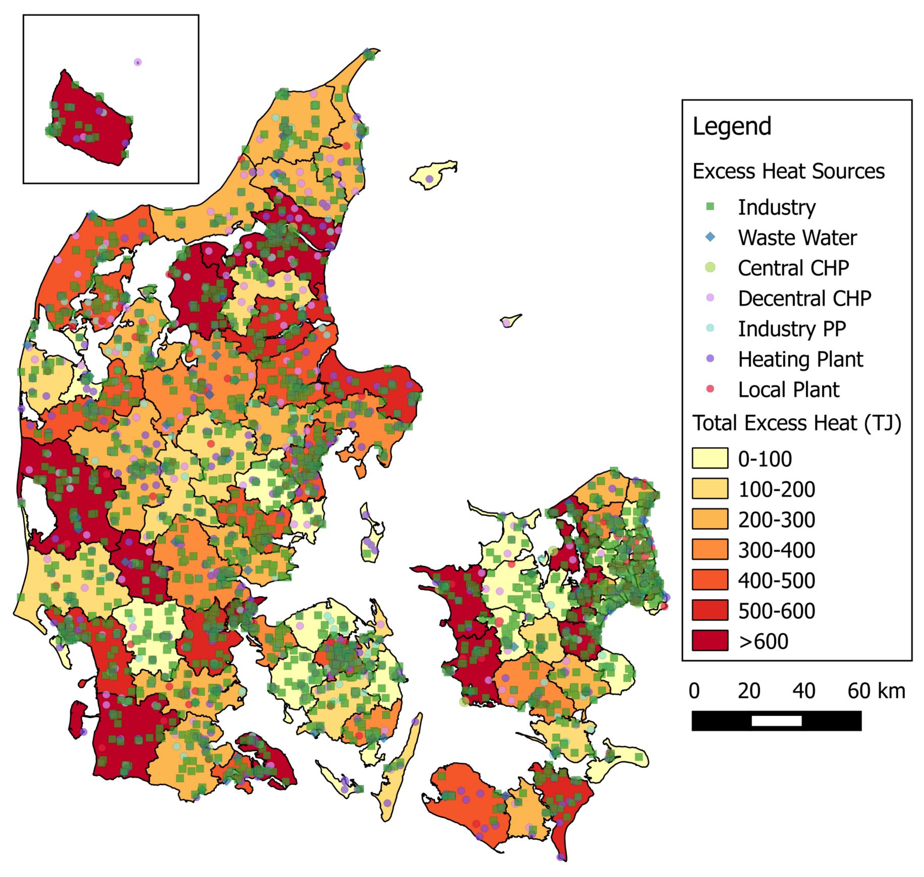
Figure 3 shows Denmark with the individual excess heat sources marked as a point layer and the sum of the excess heat in each Danish municipality indicated by a color gradient. An overview of the data used can be obtained from this figure, as all sites with a possible excess heat source are shown. This includes site that already utilize excess heat, but where more usable excess heat is expected. It can be further seen that the highest excess heat potentials were found in Aalborg, Kalundborg and Fredericia, where heavy industry is located. The greater Copenhagen area, located in the very east of Denmark, has a high density of sources, but a comparably low excess heat potential, as there is no heavy industry.
3.2. Identification and Analysis of Recovery Scenarios
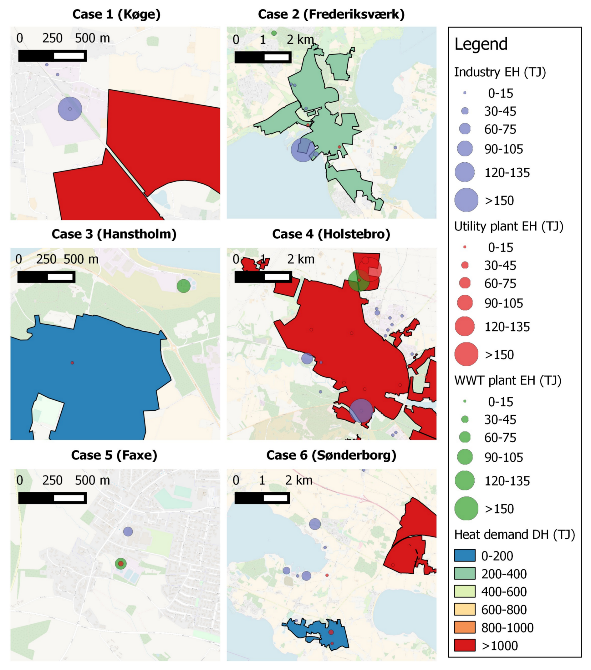
Based on the overall mapping as shown in Section 3.1, six cases of EH sources were identified, which were used as case studies for further investigation. Figure 4 shows the excess heat sources and district heating areas for selected areas. The EH sources and heat sinks were chosen to present relevant scenarios for further discussion, and four of them are based on previous works [23]. The six cases were used to investigate different EH sources and utilization pathways. Cases 1, 2 and 4 show large excess heat sources from industrial processes near district heating areas. Case 3 shows an excess heat source from a WWT plant close to a DH area, and Case 5 shows a utility plant (WWT and power plant) close to an industrial site. Lastly, Case 6 shows several large excess heat sources, from the building material industry without a nearby heating area. The information that was extracted from the GIS data are shown in Table 5 for the EH sources and in Table 6 for the possible EH users. In the following, each study is further characterized in more detail with respect to the excess heat source and heating demand, as well as the economic potential for utilizing the excess heat.
3.2.1. Case 1 (Køge)
In the first case study, the supply of excess heat to a DH area was analyzed. The temperature level of the excess heat was too low and did not allow a direct heat exchange and therefore required the use of a heat pump. The considered heat sources were from a chemical factory, which originated from evaporation, compression and refrigeration processes [27]. Temperatures of these processes are generally relatively low and were found in the range of 40 C–100 C. In the specific case study, an overall excess heat potential of 150 TJ per year was found. A detailed analysis of the source revealed that approximately 10 TJ were available at 80 C from a single distillation column on site. The production had three shifts and was considered evenly distributed throughout the year following production profile P1. The heating demand of the local DH area (Køge bay area) was more than 9670 TJ per year with a supply temperature of 85 C in winter. With the temperatures given in Table 5 and Table 6, values between 10 and 14 were achieved for the COP. The local DH area is connected to the Copenhagen DH network. Most of this heat was supplied by central combined heat and power plants, of which 400 MW were from three waste incineration plants, which are politically prioritized [65]. The choice of the district heating profile depends on the agreement found with the local authorities and how much of the existing summer capacity could be reduced. As the estimated excess heat source was small, compared to the total network capacity, the first district heating profile (DH1) was chosen.
3.2.2. Case 2 (Frederiksværk)
The second case study analyzed the supply of excess heat to a DH area, where the temperature level of the excess heat was sufficient to allow a direct heat exchange throughout the year. In the specific case, a metal processing industry was chosen, which lies within an existing DH area. In this industry, the majority of the excess heat originated from heating, melting and compression. The current mapping estimated that more than 150 TJ of EH were available per year. The specific site manufactured steel plates, where a high share of thermal energy was used for the heating of the metal, before being formed. It was assumed that 15 TJ were accessible at a temperature of 180 C. The local DH area of Frederiksværk had a heating demand of 397 TJ per year and, in winter, had a supply temperature of 80 C. As it is a smaller DH area currently supplied by a biomass boiler (wood chips and pellets), the DH Profile 1 was chosen. The steel plates were produced in three shifts and, to account for demand fluctuations, production profile P2 was chosen.
3.2.3. Case 3 (Hanstholm)
In this case study, a WWT plant is located in the vicinity of a small DH area. The WWT plant received residential sewage, but to a large part also waste water from a neighboring indoor fish farm. The temperature of the water leaving the WWT plant had a varying temperature over the year. In Denmark, this temperature typically varies between 10 C and 20 C [57]. For the analysis of the given case study, the temperature was varied over the four seasons using 10 C for winter, 20 C in summer and 15 C in spring and autumn. This was a conservative estimate for this specific case: a more constant temperature than in other WWT plants could be expected, due to the high share of input of industrial waste water. The Hanstholm DH network had a comparable low supply temperature in winter of only 73 C and was supplied by a biomass boiler, an electric boiler used for load balancing, an oil/gas boiler with a HP for the exhaust gas and EH from a fish meal factory [66]. It was assumed that with the current supply in EH and from the electric boiler, the summer heating load was covered; thus, the profile DH2 was chosen. The obtainable COPs for the heat pump were between 4.5 and 5.3.
3.2.4. Case 4 (Holstebro)
This case study was similar to Case 1, where EH could be utilized with an HP for district heating. In this case, the EH originated from a large site processing food, dairy products in particular, and was available at 60 C in the exhaust gases of dryers. Other possible EH sources were available at the site, e.g., exhaust gases from the steam boilers and gas burners, as well as from refrigeration plants, which could also be taken into consideration. The production at the dairy site took place in three shifts evenly distributed over the year. The DH demand in Holstebro was covered primarily by a CHP plant using waste and biomass. For the DH temperatures given in Table 6, a COP of up to 10 could be expected.
3.2.5. Case 5 (Faxe)
The use of excess heat as a heat source for another industrial facility was analyzed as part of the fifth case study. The industrial excess heat in this case could be used as process heat, by using either a heat pump or direct heat exchange. A possible scenario was found in the map, where almost 50 TJ of excess heat was available from the food industry and approximately 65 TJ from a WWT plant. This plant used a biogas engine to produce heat and power for internal use in the digester. The engine had a capacity of 0.5 MW and 10 MW. As there was no existing larger DH area, the excess heat could be used for local industries.
The industrial site for the food production had an estimated heating demand of 20 TJ with a temperature of 80 C for heating and cooking. The production was chosen to follow a two-shift operation and production profile P1. The excess heat from the biogas engine at a WWT plant was found to be at 110 C based on the GIS model with an accessible potential of 15 TJ per year.
3.2.6. Case 6 (Sønderborg)
In the sixth case study, the use of industrial excess heat is studied in cases where no heat demand is available and excess heat temperatures are high enough to generate electricity. The mapping identified an area west of Sønderborg, where several industries producing building material are located. There were no major heating demands present in the vicinity of the industries. The district heating areas of Sønderborg and Broager are several kilometers away. The main products of the industrial sites were bricks, and the excess heat from those was estimated to be 62 TJ, 56 TJ, 36 TJ and 12 TJ per year, respectively. As those industrial sites had similar processes, with comparable process heating demands, the exchange of heat between them was not possible. Furthermore, the closest district heating area was located more than 3 km away. In the production of bricks, the majority of excess heat originated from drying and furnaces. The exhaust gases in the brick production were typically found to range between 50 C and 80 C from the dryers and between 150 C and 250 C for the furnaces [67,68]. Already installed heat recovery systems and the use of the kiln flue gases for the dryer reduce possible process stream for further utilization. The temperature of the furnace air was chosen at the lower end as 160 C and the usable excess heat amount at 30 TJ.
3.3. Economic Analysis
The main private-economic results and their uncertainties are summarized in Table 7 for each of the case studies. The table also includes the uncertainty of each value. All case studies, except Case 3, were profitable over the assumed 20-year life time. Case 1 and Case 4 had however a low IRR, only slightly above the discount rate. Taking into account the uncertainties, these two cases could also be unprofitable, as the standard deviation exceeded the positive NPV. Case 3 presented the highest investment costs, because a heat pump was required for a large low-temperature EH source.
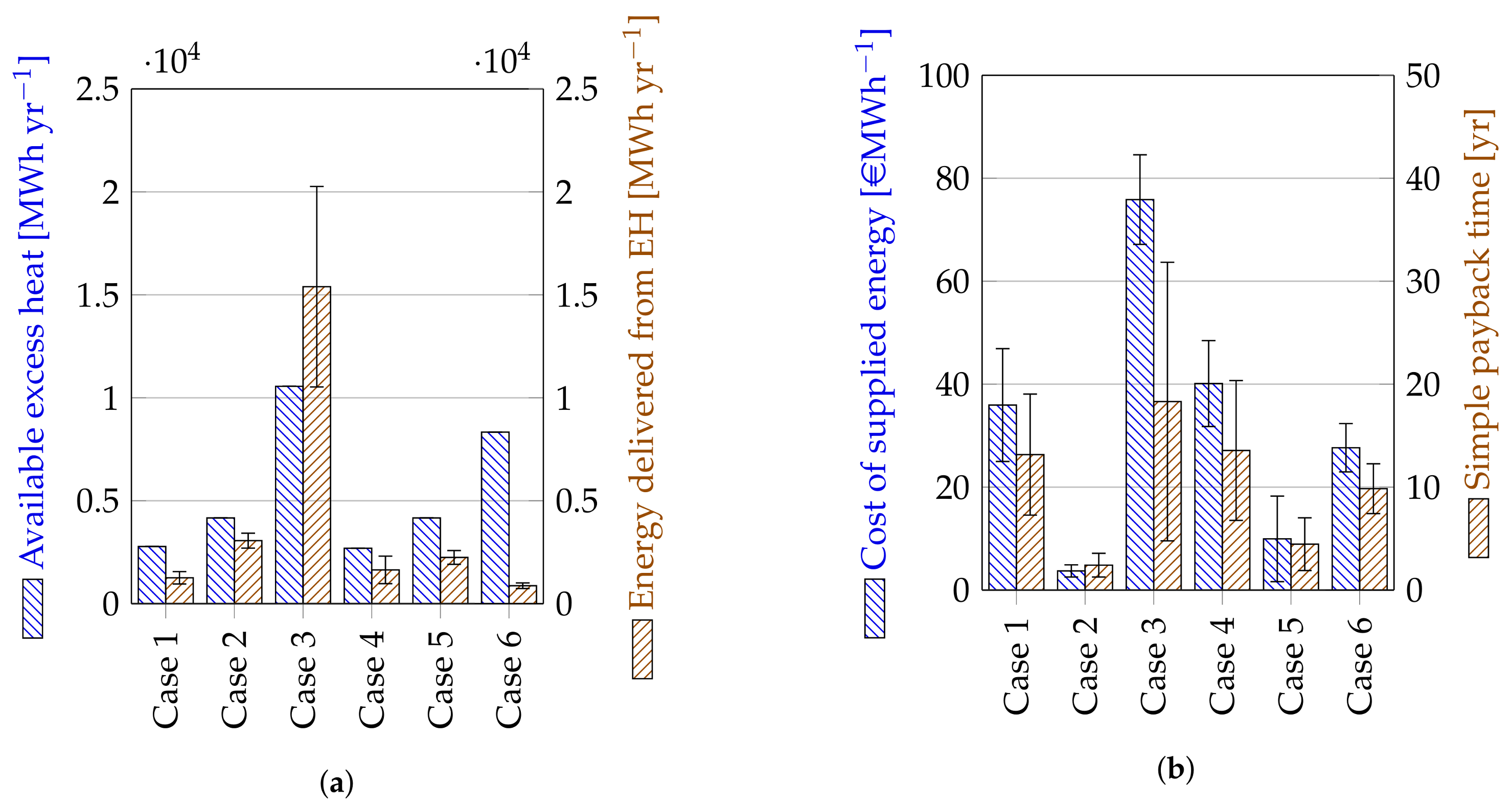
In Figure 5, the case studies are compared by showing the available and recovered energy (Figure 5a) and their unit costs, as well as simple payback time of the investment (Figure 5b). Most cases could not recover the entire assumed EH, which was due to a limited demand (Case 4) or due to remaining excess heat in the source ().
The unit costs of industrial EH utilization with a heat pump were less than 40 € per MWh and considerably higher than for the direct utilization (Case 2). The heating price of utilizing waste water for district heating had a high heating price of 76 € per MWh, with a low relative uncertainty. For the given Case Study 3, this investment would only be acceptable if the lifetime was high (above 20 years) and no less expensive renewable heat sources were available in the given heating area. The presented simple payback time only took into account economic feasible investment (revenues larger than the operating costs) obtained in the MC simulations and could thus only be meaningful in combination with the other indicators. Though the mean simple payback times were generally below 20 years, they were often too high for private economic investments where payback times of under five years are required.
Case Study 6, where electricity was generated from EH, had a low unit cost compared to the net electricity price. The NPV over 20 years was with 283,000 € relatively low, but the uncertainty of the IRR and the other indicators was acceptable. In Case Study 3, the reason for the increased uncertainty was that the uncertainty of the excess heat temperature of the gaseous source in some uncertainty estimations caused the use of a heat pump, which had a great impact on the heat delivered, investment costs and operating costs. This was also shown in the sensitivity analysis, where the excess heat temperature for Case 3 had an over proportional influence.
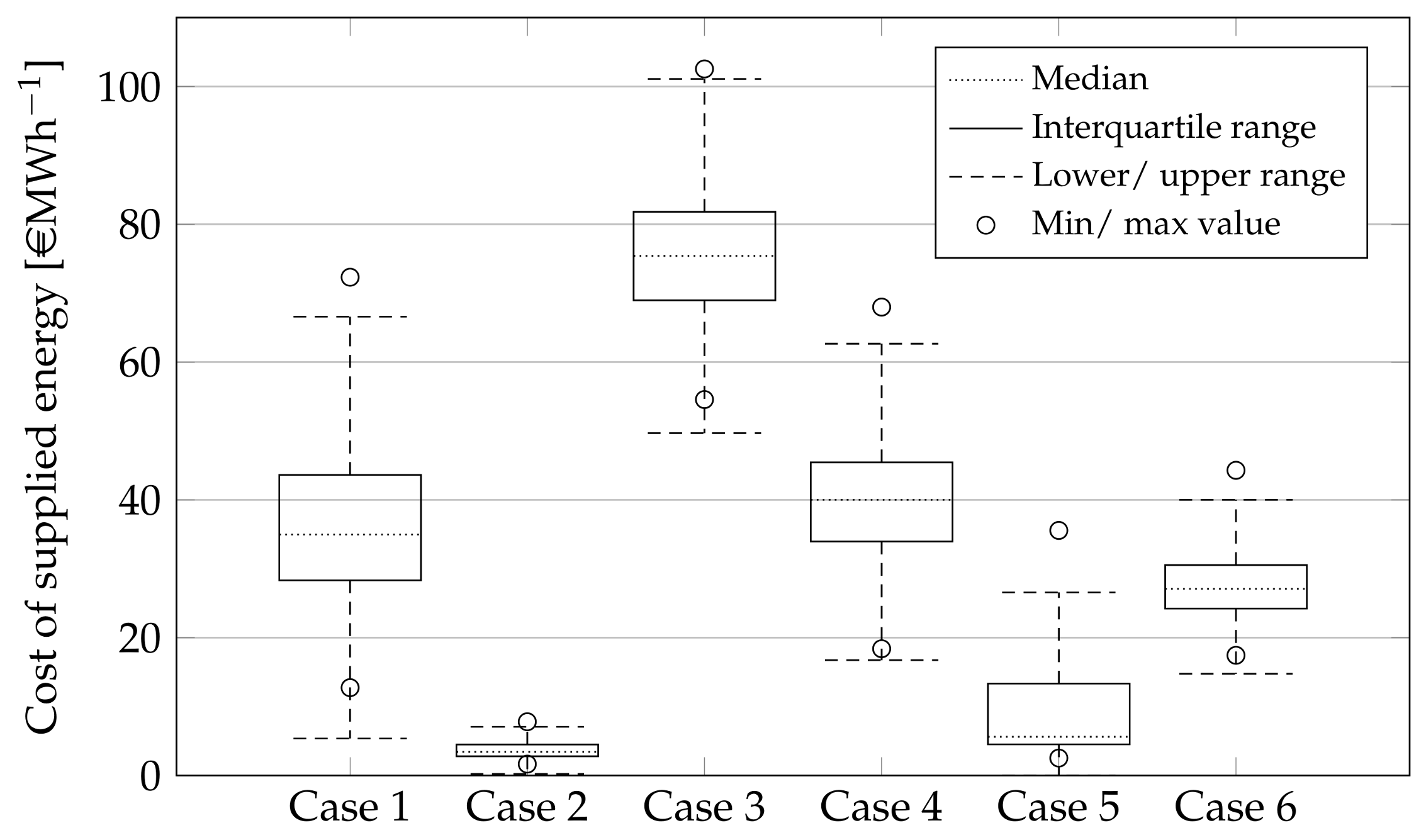
Figure 6 shows the box plot of the costs for the supplied energy for each case. The bottom and top of each box represent the first and third quartiles of the distribution respectively. The whiskers extend to represent the values, which fell within 1.5-times the interquartile range (third minus the first quartile). For Case 1, it can be observed that almost 75% of the lowest MC simulations fell below the average DH price of 40.5 € per MWh. This suggests with a high certainty that the heat from the EH source could be supplied at costs lower than the current ones. A more detailed analysis of Case 1 is thus justified.
Case 5 had a very uneven distribution of the MC simulations, with the median value being very close to the first quartile. There was furthermore a large dispersion of the possible costs in the upper half of the data. The main reason for this was the criteria for the subsidy, which should not bring the simple payback time below one year. As Case 5 had a good economy, it often did not qualify for the subsidy in the simulations. However, as soon as it qualified for the subsidy, the uncertainty of the parameters used to calculate the subsidy was added. Thus, the higher costs of supplied energy were more scattered. The lower and upper ranges encompass considerably larger ranges than indicated by the standard deviations shown in Figure 5b. For Case 6, the highest outlier is in the same range as for Case 5, which was not obvious from the standard deviations. When comparing the spread of the values, as shown in the box plots, a better comparison of different alternatives would be possible.
3.4. Sensitivity Analysis
The NPV was chosen as the model output to analyze the impact of the uncertain parameters, as the calculation of the NPV included all of them. Based on the two methods described in Section 2.5, linear regression and Morris screening, a ranking of the most influential parameters was performed. The sensitivity indicator, absolute SRC and * are presented in Table 8 and Table 9 for the respective five highest scoring parameters. The R values for the linearization of the MC simulations were between 0.75 and 0.95, indicating that sufficient linearization was possible to use the results.
This ranking reveals that all cases generating district heat had the district heating price, increase in DH price and profit share between EH emitter and DH operator as very influential parameters. In the ORC case, the electricity price and electricity price increase were determined as the most important parameter. These parameters all had a direct impact on the NPV and were identified as important using both sensitivity methods. In Case Studies 1 and 5, the excess heat temperature was identified as another important parameter, as it decided in these cases if a HP was required for the utilization. On the other hand, in Case 3, the heat pump efficiency was important. Here, the COP was low, and thus, the efficiency had a high impact on the electric energy use.
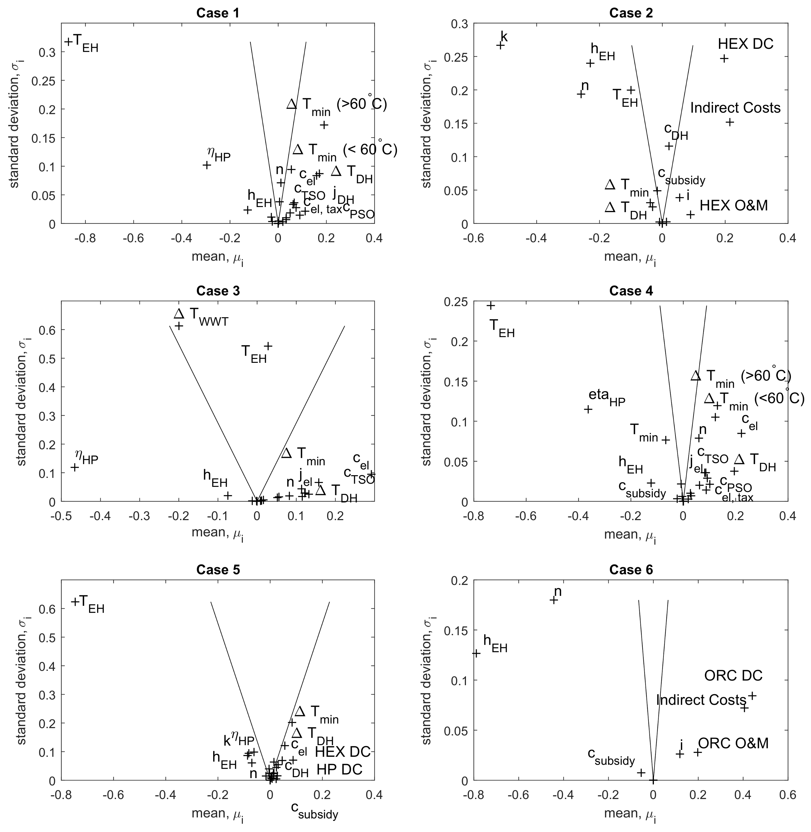
To analyze the significance of the parameters on the costs of supplied energy and present more parameters, the results of the Morris screening are shown graphically in Figure 7 for each case. The lines in each graph represent the mean value +/− the standard deviation divided by the square root of the repetitions [69]. Points lying outside of the lines have significant impact on the output. If the points are to the right of the curve, they increase the value of the results and vice versa. Parameters with a high absolute mean value have a high significance for the model, whereas a high standard deviation represents high interactions of the parameter. For Cases 1–5, the EH temperature and the heat pump efficiency or heat transfer coefficient had a high mean and standard deviation. The minimum temperature differences could have a high impact if the system requires a heat pump, then also the costs related to the electricity were important. The variations of the value for the sale of energy savings, as part of the subsidy, had usually no impact on the result. For the ORC case, the main influential factors were the annual operating hours, lifetime and costs directly related to the ORC investment.
3.5. Environmental Considerations
An analysis, considering environmental aspects, can give additional insights and allow for a better comparison of alternatives. With the data implemented in the GIS model, such an analysis is possible. Potential conflicts with current heat producers can be identified, together with environmental benefits. The possibilities are shown for the examples of Case Study 1 and Case Study 2.
The proposed utilization pathway in Case 1 would supply heat to the district heating network of greater Copenhagen. The network is currently supplied with heat originating from several central combined heat and power plants. These plants are using biomass (wood chips and pellets) or are in the transition of substituting coal with biomass. The delivered district heating from the chemical factory would decrease the required heat supply from existing sources by less than 0.2%. This reduction is expected to have a negligible impact on the power production.
The district heating network, associated with Case Study 2, had 84% of the heating demand covered by wood chips, 13% by natural gas and 3% by bio oil fired in one heating plant. The substitution of some of these fuels with excess heat would thus not impact the electricity production. The emissions of CO would not be reduced significantly, as most of the district heat was supplied from biomass, and the excess heat originates from burned natural gas.
4. Discussion
The excess heat used for the geographical mapping was based on aggregated numbers, which were allocated to production sites and grouped excess heat from different sources. The excess heat found for a given geographical location may thus originate from several sources. It is thus required to carefully analyze any match and the spatial vicinity of the point sources to find the real potential of excess heat and heating demand. The assessment can be supported with information from the literature, with which the first estimate of the excess heat sources can be improved. It should further be carefully evaluated if there are any opportunities for heat integration on site or if a reduction of the excess heat through better equipment and process control is possible. This would often be favored, before an external utilization is considered. This aspect was not included in the present study, but it was assumed that an internal assessment has already been made or would be made prior to performing a detailed feasibility study.
Several studies identified large technical potentials for the external utilization of excess heat. These potentials mainly refer to DH and some potential for electricity generation. However, these potentials are not realized, i.e., excess heat constitutes only 2% of the Danish district heating production. One of the main reasons for this gap is the lack of business models and common practice. The common practices keep industries and district heating companies within their core business areas, i.e., investing into known technologies (e.g., DH boilers). At the same time, the external utilization of excess heat could be the most beneficial for both sides.
For the economic analysis, key figures were used to estimate the costs for the given system, without performing a detailed technical evaluation of component sizes and their costs. The aim of the economic evaluation was to give an overview of the feasibility and should be applicable for the evaluation of a large number of cases. This quick evaluation should not require the specification of additional parameters, other than the ones already added to the model of data from the general literature. If a match is found to be feasible, considering the determined uncertainties, a more detailed evaluation has to be undertaken. Such an additional evaluation should include the analysis of the possibly required thermal storage tanks for daily load and demand variations, a detailed analysis of the industrial processes on site and how the excess heat can be utilized. The sensitivity analysis identified the most important parameters, which should be quantified and selected carefully. The investment costs, heat pump efficiency, the annual operating hours, accessible excess heat amount and temperature were found to be particularly important. The substitution price of the district heating has an impact on the final economic economic. This price depends on the local energy system and the agreements between the owner of the excess heat and the utility company. If the utilization of excess heat proves to be economically feasible, it needs to be clarified how the profit should be split. In the present tool, the assumption was that the industrial plant will get 75% of the profit and the district heating company the remaining 25%. This distribution will be different in reality and depends on the result of negotiations, the involved risks, interests and best technical solution.
A comparison of the costs with other literature values shows that the assumptions and order of magnitude of the results in this work are comparable. Karner et al. [16] found, for two case studies in Austria, costs for urban heating from industrial excess heat between 27 and 38 € per MWh and average amortization times of seven years. Eriksson et al. [15] found a heat sale price of 20 € per MWh for a case in Sweden. In Denmark, several projects are documented where DH is supplied by large heat pumps [70]. For the combined supply of DH and cooling, heating costs of 55 € per MWh (simple payback time of 4.6 years) in one project and 47 € per MWh (simple payback time below three years) in another one were obtained. A price of 30 € per MWh was given to another project, where industrial EH is used for DH. These costs for EH utilization are comparable to the ones found in this work, but also show the large variations that arise from different characteristics of each case. There is thus a necessity for an initial evaluation and comparison of possible cases, taking the most important characteristics into account. Considering this, the presented tool will allow the managers of DH companies and industries to analyze potential synergies, i.e., allowing DH companies and industries to become aware of the cooperation possibilities. If the cooperation proves to be economically feasible (low payback time) with acceptable uncertainty, a detailed analysis should be conducted. If the calculated uncertainty is too high, the cases could be re-evaluated using the tool, but with more robust input parameters. If the economic indicators are poor, there is no need for additional analyses.
The methodology in this work was developed with data available in Denmark and took into consideration the local taxes and regulations. While the taxes and regulations can easily be adjusted to other countries, data on excess heat sources and district heating networks may be limited and would require additional empirical studies.
In order to improve the model output, the profit share between the EH emitter and the EH user needs to be more certain, as it has a high impact on the overall evaluation. By creating generally applicable business models or referring to previous accomplished cases, this value can be refined, but will still depend on final negotiations. Though the DH price in a given DH area is known, the substitution price might be different or change with future investments. The EH temperature needs to be carefully chosen, in particular when it is close to the heating demand temperature, as small differences will impact the requirement of a heat pump and thus the investment and operating costs.
5. Conclusions
This work presented a method to identify, analyze and evaluate cases for utilizing excess heat. The method is based on a geographical mapping in GIS, where excess heat sources from the industry and utility sector, as well as heating demands are shown. The GIS mapping was used to identify specific cases where excess heat could be utilized externally for heating purposes or electricity production. Using a developed model for a fast economic and technical evaluation of potential matches, the feasibility of the matches was evaluated. The approach of using the GIS model in combination with economic and technical analysis is suitable to identify local synergies. This has a particular relevance for energy planners, DH operators and industry representatives, who get the possibility to analyze investment opportunities with readily-available data and first assumptions.
In the second step, an uncertainty and sensitivity analysis was performed for each case, which can be used to better assess the model results and refine the input data and assumptions. The six case studies evaluated in this paper considered industrial EH and waste water for district heating, as well as EH from a utility to an industrial plant and lastly industrial EH for electricity generation. It was shown that the costs of the supplied heat were below the average DH prices, except for the EH from WWT. The IRR for the feasible cases ranged from 7–54% and depended considerable on whether a heat pump was used or not. The reported uncertainties of the mean values, found with the Monte Carlo method, show an acceptable uncertainty, which allows a first decision on projects’ feasibility. The sensitivity analyses identified several critical parameters, which must be carefully chosen. The price obtainable for the generated heat, as well as the share of the profit between the EH emitter and the owner of the heat demand have a great influence on the project’s economy (i.e., IRR and NPV). A detailed evaluation of possible business models for synergies is required, which would reduce the uncertainty of these values before detailed negotiations. The costs of the recovered heat are primarily influenced by the excess heat temperature. In particular, when the required sink temperature is close to the EH temperature, the uncertainty increases, as the use of a heat pump might be required with corresponding increases in cost.
Author Contributions
Fabian Bühler developed the tool, performed the simulations and wrote the manuscript. Stefan Petrovic helped with analyzing the data, GIS modeling and revising the manuscript. Fridolin Müller Holm contributed to the taxes and subsidies, as well as the case studies. Torben Ommen, Henrik Pieper and Brian Elmegaard revised the manuscript and provided important recommendations; all authors read and approved the final manuscript.
Conflicts of Interest
The authors declare no conflict of interest.
Abbreviations
The following abbreviations are used in this manuscript:
| AF | Annuity factor |
| COP | Coefficient of performance |
| DC | Direct costs |
| DH | District heating |
| EE | Elementary effects |
| EH | Excess heat |
| fct | Function |
| G | Gamma |
| GHG | Greenhouse gas |
| GIS | Geographical information systems |
| HP | Heat pump |
| HEX | Heat exchanger |
| IRR | Internal rate of return |
| LHS | Latin hypercube sampling |
| MC | Monte Carlo |
| N | Normal |
| NPV | Net present value |
| O&M | Operation and maintenance |
| ORC | Organic Rankine cycle |
| P | Production profile |
| PP | Power plant |
| PEC | Purchased equipment costs |
| SEK | Svensk krone (Swedish Krona) |
| SRC | Standardized regression coefficient |
| TCI | Total capital investment |
| U | Uniform |
| WWT | Waste water treatment |
| Nomenclature | |
| a | Shape parameter (-) |
| b | Inverse scale parameter (-) |
| c | Unit costs (€ MWh) |
| CRF | Capital recovery factor (-) |
| d | Discount rate (%) |
| h | Operating hours (h) |
| i | Interest rate (%) |
| I | Investment costs (€) |
| j | Annual price increase (%) |
| k | Overall heat transfer coefficient (W·mK) |
| n | Lifetime (years) |
| p | Perturbation (-) |
| Q | Heat flow (TJ) |
| r | Repetitions (-) |
| S | Share (-) |
| T | Temperature (K) or (C) |
| Greek Letters | |
| Absolute difference (-) | |
| Efficiency (-) | |
| Mean (-) | |
| Absolute mean (-) | |
| Standard deviation (-) | |
| Sub- and Super-scripts | |
| 0 | Reference point, ambient |
| E | Equipment |
| EH | Excess heat |
| el | Electric |
| f | Fixed |
| H | Heating |
| HD | Heating Demand |
| L | Loan |
| min | Minimum |
| P | Profit |
| R | Return |
| S | Supply |
| Su | Summer |
| v | Variable |
| W | Winter |
References
- Jaffe, A.B.; Stavins, R.N. The energy-effincency gap What does it mean? Energy Policy 1994, 22, 804–810. [Google Scholar] [CrossRef]
- Pehnt, M.; Bödeker, J.; Arens, M.; Jochem, E.; Idrissova, F. The Utilisation of Industrial Excess Heat—Techno-Economic Potentials and Energy Policitcal Realisation. Die Nutzung Industrieller Abwärme—Technisch-Wirtschaftliche Potentiale und Energiepolitische Umsetzung. 2010. Available online: http://www.my-e-drive.de/energie/pdf/Nutzung_industrieller_Abwaerme.pdf (accessed on 1 March 2018). (In Danish).
- Walsh, C.; Thornley, P. Barriers to improving energy efficiency within the process industries with a focus on low grade heat utilization. J. Clean. Prod. 2012, 23, 138–146. [Google Scholar] [CrossRef]
- Broberg Viklund, S. Energy efficiency through industrial excess heat recovery—Policy impacts. Energy Effic. 2015, 8, 19–35. [Google Scholar] [CrossRef]
- Miró, L.; Brückner, S.; Cabeza, L.F. Mapping and discussing Industrial Waste Heat (IWH) potentials for different countries. Renew. Sustain. Energy Rev. 2015, 51, 847–855. [Google Scholar] [CrossRef]
- Naegler, T.; Simon, S.; Klein, M.; Gils, H.C. Quantification of the European industrial heat demand by branch and temperature level. Int. J. Energy Res. 2015, 39, 2019–2030. [Google Scholar] [CrossRef]
- Brückner, S.; Miró, L.; Cabeza, L.F.; Pehnt, M.; Laevemann, E. Methods to estimate the industrial waste heat potential of regions—A categorization and literature review. Renew. Sustain. Energy Rev. 2014, 38, 164–171. [Google Scholar] [CrossRef]
- Miró, L.; McKenna, R.; Jäger, T.; Cabeza, L.F. Estimating the industrial waste heat recovery potential based on CO2 emissions in the European non-metallic mineral industry. Energy Effic. 2017, 17. [Google Scholar] [CrossRef]
- McKenna, R.C.; Norman, J.B. Spatial modeling of industrial heat loads and recovery potentials in the UK. Energy Policy 2010, 38, 5878–5891. [Google Scholar] [CrossRef]
- Persson, U.; Möller, B.; Werner, S. Heat Roadmap Europe: Identifying strategic heat synergy regions. Energy Policy 2014, 74, 663–681. [Google Scholar] [CrossRef]
- Brückner, S.; Schäfers, H.; Peters, I.; Lävemann, E. Using industrial and commercial waste heat for residential heat supply: A case study from Hamburg, Germany. Sustain. Cities Soc. 2014, 13, 139–142. [Google Scholar] [CrossRef]
- Brückner, S.; Liu, S.; Miró, L.; Radspieler, M.; Cabeza, L.F.; Lävemann, E. Industrial waste heat recovery technologies: An economic analysis of heat transformation technologies. Appl. Energy 2015, 151, 157–167. [Google Scholar] [CrossRef]
- Broberg, S.; Backlund, S.; Karlsson, M.; Thollander, P. Industrial excess heat deliveries to Swedish district heating networks: Drop it like it’s hot. Energy Policy 2012, 51, 332–339. [Google Scholar] [CrossRef]
- Viklund, S.B.; Johansson, M.T. Technologies for utilization of industrial excess heat: Potentials for energy recovery and CO2 emission reduction. Energy Convers. Manag. 2014, 77, 369–379. [Google Scholar] [CrossRef]
- Eriksson, L.; Morandin, M.; Harvey, S. A feasibility study of improved heat recovery and excess heat export at a Swedish chemical complex site. Int. J. Energy Res. 2017, 2, 1–14. [Google Scholar] [CrossRef]
- Karner, K.; Theissing, M.; Kienberger, T. Modeling of energy efficiency increase of urban areas through synergies with industries. Energy 2017, 136, 201–209. [Google Scholar] [CrossRef]
- Li, Y.; Xia, J.; Su, Y.; Jiang, Y. Systematic optimization for the utilization of low-temperature industrial excess heat for district heating. Energy 2018, 144, 984–991. [Google Scholar] [CrossRef]
- Hammond, G.P.; Norman, J.B. Heat recovery opportunities in UK industry. Appl. Energy 2014, 116, 387–397. [Google Scholar] [CrossRef]
- Cooper, S.J.G.; Hammond, G.P.; Norman, J.B. Potential for use of heat rejected from industry in district heating networks, Gb perspective. J. Energy Inst. 2016, 89, 57–69. [Google Scholar] [CrossRef]
- Lund, R.; Persson, U. Mapping of potential heat sources for heat pumps for district heating in Denmark. Energy 2016, 110, 129–138. [Google Scholar] [CrossRef]
- Bühler, F.; Petrović, S.; Karlsson, K.; Elmegaard, B. Industrial excess heat for district heating. Appl. Energy 2017, 205, 991–1001. [Google Scholar] [CrossRef]
- Bühler, F.; Petrović, S.; Holm, F.M.; Karlsson, K.; Elmegaard, B. Spatiotemporal and economic analysis of industrial excess heat as a resource for district heating. Energy 2018, in press. [Google Scholar]
- Bühler, F.; Petrović, S.; Ommen, T.; Müller Holm, F.; Elmegaard, B. Identification of Excess Heat Utilisation Potential using GIS: Analysis of Case Studies for Denmark. In Proceedings of the 30th International Conference on Efficiency, Cost, Optimisation, Simulation (ECOS), San Diego, CA, USA, 2–6 July 2017; pp. 1–16. [Google Scholar]
- Bühler, F.; Nguyen, T.V.; Elmegaard, B. Energy and exergy analyses of the Danish industry sector. Appl. Energy 2016, 184, 1447–1459. [Google Scholar] [CrossRef]
- Denmark Statistics. ENE2HA: Energy Account in Common Units (Detailed Table) by Use and Type of Energy. 2017. Available online: www.statistikbanken.dk/ENE2HA (accessed on 30 October 2017).
- Danish Energy Agency; Viegand Maagøe A/S. Mapping of Energy Use in the Companies. Kortlægning af Energiforbrug I Virksomheder. 2015. Available online: http://www.ens.dk/forbrug-besparelser/ (accessed on 25 March 2018). (In Danish)
- Bühler, F.; Holm, F.; Huang, B.; Andreasen, J.; Elmegaard, B. Mapping of low temperature heat sources in Denmk. In Proceedings of the ECOS 2015-28th International Conference on Efficiency, Cost, Optimization, Simulation and Environmental Impact of Energy Systems, Pau, France, 29 June–3 July 2015. [Google Scholar]
- Danish Energy Agency. Energy Producers Count. Energiproducenttælling 2010–2012. 2014. Available online: https://ens.dk/service/statistik-data-noegletal-og-kort/ (accessed on 1 March 2018). (In Danish)
- Danish Environmental Protection Agency. Environmental Data (Miljødata). 2016. Available online: http://www2.mst.dk/blst_databaser/mstmiljoedata (accessed on 1 January 2017).
- Erhvervsstyrelsen. PlansystemDK. 2016. Available online: http://kort.plansystem.dk/spatialmap (accessed on 4 January 2017).
- Danish District Heating Association. Dansk Fjernvarmes Årsstatistik 2015/2016 [Annual District Heating Statistics 2015/2016]. 2016. Available online: www.danskfjernvarme.dk/viden-om/aarsstatistik/statistik-2015-2016 (accessed on 1 March 2017).
- QGIS Development Team. QGIS Geographic Information System. Open Source Geospatial Foundation Project. 2016. Available online: http://www.qgis.org/ (accessed on 25 March 2018).
- Contributors, O. Planet Dump. Available online: http://planet.openstreetmap.org/ (accessed on 1 March 2018).
- Jensen, J.K.; Ommen, T.; Markussen, W.B.; Elmegaard, B. Design of serially connected ammonia-water hybrid absorption-compression heat pumps for district heating with the utilization of a geothermal heat source. In Proceedings of the 29th International Conference on Efficiency, Cost, Optimisation, Simulation and Environmental Impact of Energy Systems, Portoroz, Slovenia, 19–23 June 2016. [Google Scholar]
- Ommen, T.; Markussen, W.B.; Elmegaard, B. Heat pumps in combined heat and power systems. Energy 2014, 76, 989–1000. [Google Scholar] [CrossRef]
- Johansson, M.T.; Söderström, M. Electricity generation from low-temperature industrial excess heat-an opportunity for the steel industry. Energy Effic. 2014, 7, 203–215. [Google Scholar] [CrossRef]
- Sørensen, P.A.; Paaske, B.L.; Jacobsen, L.H.; Hofmeister, M. Report Concerning Thermal Storage Technologies and Large Heat Pumps for the Use in District Heating Networks. Udredning Vedrørende Varmelagringsteknologier Og Store Varmepumper I Fjernvarmesystemet. 2013. Available online: https://ens.dk/sites/ens.dk/files/Forskning_og_udvikling/udredning_om_varmelagringsteknologier_og_store_varmepumper_i_fjernvarmesystemet_nov_2013.pdf (accessed on 1 March 2018). (In Danish).
- Danish Energy Agency. Technology Data for Energy Plants—Generation of Electricity and District Heating, Energy Storage and Energy Carrier Generation and Conversion. 2015. Available online: https://ens.dk/en/our-services/projections-and-models/technology-data (accessed on 1 March 2018).
- Nielsen, S.; Müller, B. GIS based analysis of future district heating potential in Denmark. Energy 2013, 57, 458–468. [Google Scholar] [CrossRef]
- Bejan, A.; Tsatsaronis, G.; Moran, M. Thermal Design and Optimization; Wiley-Interscience: New York, NY, USA, 1996. [Google Scholar]
- Danish Energy Regulatory Authority. Heating Price Statistics. In Danish: Varmeprisstatistik; Technical Report; Danish Energy Regulatory Authority: Copenhagen, Denmark, 2016. [Google Scholar]
- Ea Energianalyse. District Heating Analysis—Supplementary Report. In Fjernvarmeanalyse-Bilagsrapport; Technical Report; Ea Energianalyse: Copenhagen, Denmark, 2014. (In Danish) [Google Scholar]
- Danish Energy Agency. Data, Tables, Statistics and Maps, Energy in Denmark. 2015. Available online: https://ens.dk/service/statistik-noegletal-og-kort/energipriser-og-afgifter (accessed on 1 March 2018).
- Danish Energy Agency. Socioeconomic cAlculation Basis for Energy Prices and Emissions. Samfundsøkonomiske Beregningsforudsætninger for Energipriser Og Emissioner. 2017. Available online: https://ens.dk/sites/ens.dk/files/Analyser/samfundsoekonomiske_beregningsforudsaetninger_2017.pdf (accessed on 1 March 2018). (In Danish)
- Energinet.dk. Current, Future and Historic Tariffs and Fees. Aktuelle, Kommende Og Historiske Tariffer Og Gebyrer. 2017. Available online: https://energinet.dk/El/Tariffer (accessed on 12 December 2017). (In Danish).
- Dansk Fjernvarme. Benchmarking Statistic 2014/2015. 2015. Available online: http://www.danskfjernvarme.dk/viden-om/aarsstatistik/benchmarking-statistik-2014-2015 (accessed on 1 March 2018).
- Danish Tax Authority (SKAT). Legal Instructions 2016-2 E.A.4 Energy. Den Juridiske Vejledning 2016-2 E.A.4 Energi. 2016. Available online: http://www.skat.dk/SKAT.aspx?oId=1921342{&}chk=212649 (accessed on 25 March 2018). (In Danish)
- Danish Tax Authority (SKAT). Legal Instructions 2016-2 E.A.7 Environment. Den Juridiske Vejledning 2016-2 E.A.7 Miljø]. 2016. Available online: http://www.skat.dk/SKAT.aspx?oId=1921345{%}7B{&}{%}7Dchk=212649 (accessed on 25 March 2018). (In Danish)
- Finansministeriet. Aftale Mellem Regeringen, Dansk Folkeparti, Liberal Alliance og Det Konservative Folkeparti ERHVERVS- OG IVÆRKSÆTTERINITIATIVER af 12. November 2017; Technical Report; Finansministeriet: Copenhagen, Denmark, 2017. [Google Scholar]
- Danish Energy Agency. Agreement of December 16th, 2016 on the Energy Companies’ Energy Savings Effort between the Minister for Energy, Utilities and Climate and the Network and Distribution Companies within the Fields of Electricity, Natural Gas, District Heating and Oil; Technical Report; Danish Energy Agency: Copenhagen, Denmark, 2016.
- Metropolis, N.; Ulam, S. The Monte Carlo Method. J. Am. Stat. Assoc. 1949, 44, 335–341. [Google Scholar] [CrossRef] [PubMed]
- Helton, J.C.; Davis, F.J. Latin hypercube sampling and the propagation of uncertainty in analyses of complex systems. Reliab. Eng. Syst. Saf. 2003, 81, 23–69. [Google Scholar] [CrossRef]
- Sin, G.; Gernaey, K. Data Handling and Parameter Estimation. In Experimental Methods in Wastewater Treatment; van Loosdrecht, M.C., Nielsen, P., Lopez-Vazquez, C., Brdjanovic, D., Eds.; IWA Publishing Company: London, UK, 2016; Volume 9781780404, Chapter 5; pp. 201–234. [Google Scholar]
- Ommen, T.S.; Elmegaard, B.; Markussen, W.B. Heat Pumps in CHP Systems: High-Efficiency Energy System Utilising Combined Heat and Power and Heat Pumps; Technical Report; DTU Mechanical Engineering: Kongens Lyngby, Denmark, 2015. [Google Scholar]
- ØStergaard, P.A.; Andersen, A.N. Booster heat pumps and central heat pumps in district heating. Appl. Energy 2016, 184, 1374–1388. [Google Scholar] [CrossRef]
- VDI-Gesellschaft Verfahrenstechnik und Chemieingenieurwesen (GVC). VDI Heat Atlas, 2nd ed.; Springer: Berlin/Heidelberg, Germany, 2010; Volume 1. [Google Scholar]
- Clausen, K.S.; From, N.; Hofmeister, M.; Paaske, B.L.; Flørning, J. Guidelines for Large Heat Pump Projects in District Heating Systems, Drejebog Til Store Varmepumpeprojekter I Fjernvarmesystemet. 2014. Available online: https://ens.dk/sites/ens.dk/files/varme/drejebog_1.pdf (accessed on 25 March 2018). (In Danish).
- Morris, M.D. Factorial Sampling Plans for Preliminary Computational Experiments. Technometrics 1991, 33, 161–174. [Google Scholar] [CrossRef]
- Sin, G.; Gernaey, K.V.; Lantz, A.E. Good modeling practice (GMoP) for PAT applications: Propagation of input uncertainty and sensitivity analysis. Biotechnol. Prog. 2009, 25, 1043–1053. [Google Scholar] [CrossRef] [PubMed]
- Ruano, M.V.; Ribes, J.; Ferrer, J.; Sin, G. Application of the Morris method for screening the influential parameters of fuzzy controllers applied to wastewater treatment plants. Water Sci. Technol. 2011, 63, 2199–2206. [Google Scholar] [CrossRef] [PubMed]
- Saltelli, A.; Ratto, M.; Andres, T.; Campolongo, F.; Cariboni, J.; Gatelli, D.; Saisana, M.; Tarantola, S. Global Sensitivity Analysis: The Primer; John Wiley & Sons: Hoboken, NJ, USA, 2008. [Google Scholar]
- Saltelli, A.; Annoni, P.; Azzini, I.; Campolongo, F.; Ratto, M.; Tarantola, S. Variance based sensitivity analysis of model output. Design and estimator for the total sensitivity index. Comput. Phys. Commun. 2010, 181, 259–270. [Google Scholar] [CrossRef]
- Danish Energy Agency. Technology Data for Energy Plants Updated Chapters, August 2016. Available online: https://ens.dk/en/our-services/projections-and-models/technology-data (accessed on 1 March 2018).
- Dewallef, P.; Lemort, V.; Quoilin, S.; van den Broek, M. Techno-economic survey of Organic Rankine Cycle (ORC) systems. Renew. Sustain. Energy Rev. 2013, 22, 168–186. [Google Scholar]
- Varmelast.dk. Varmlast-Background for Greater Copenhagen. 2017. Available online: http://www.varmelast.dk/en (accessed on 16 January 2017).
- Hanstholm Varmeværk Amba. Hanstholm Heating Plant: Historic Overview. Hanstholm Varmeværk: Historisk Oversigt. 2015. Available online: http://www.hanstholmvarmevaerk.dk/media/2893621/historisk-oversigt.pdf (accessed on 1 March 2017). (In Danish).
- Carbon Trust. Industrial Energy Efficiency Accelerator: Guide to the Brick Sector. 2011. Available online: https://www.carbontrust.com/media/206500/ctg062-metalforming-industrial-energy-efficiency.pdf (accessed on 25 March 2018).
- Siefke, C. Utilization of Waste Heat and Combined Energy Systems in Brick Plants. Ziegelind. Int. Brick Tile Ind. Int. 2013, 66, 39–44. [Google Scholar]
- Frutiger, J.; Abildskov, J.; Sin, G. Global Sensitivity Analysis of Computer-Aided Molecular Design Problem for the Development of Novel Working Fluids for Power Cycles; Elsevier Masson SAS: Paris, France, 2016; Volume 38, pp. 283–288. [Google Scholar]
- Støchkel, H.K.; Paaske, B.L.; Clausen, K.S. Inspiration Catalogue for Large Heat Pump Projects in District Heating Systems. Inspirationskatalog for Store Varmepumpeprojekter I Fjernvarmesystemet. Technical Report. 2017. Available online: https://ens.dk/sites/ens.dk/files/varme/inspirationskatalog.pdf (accessed on 25 March 2018). (In Danish).
Figure 1.
Overview of the method for evaluating the feasibility of different cases for the EH utilization potentials.
Figure 1.
Overview of the method for evaluating the feasibility of different cases for the EH utilization potentials.

Figure 2.
Utilization pathways for excess heat from different sources.

Figure 3.
Map of Denmark with the location and type of excess heat sources and the total sum of excess heat of each region.
Figure 3.
Map of Denmark with the location and type of excess heat sources and the total sum of excess heat of each region.

Figure 4.
Examples of the identified case studies based on the overall mapping. The maps show excess heat sources as points with the radius of the points proportional to the annual excess heat. The locations of district heating areas are marked as polygons with the color representing the annual heating demand.

Figure 5.
Main results with the standard deviation as the uncertainty range. (a) Energy indicators; (b) economic indicators.
Figure 5.
Main results with the standard deviation as the uncertainty range. (a) Energy indicators; (b) economic indicators.

Figure 6.
Box plot showing the costs for supplied energy for each case study.

Figure 7.
Results of the Morris screening for the most important parameters influencing the costs of supplied energy ().
Figure 7.
Results of the Morris screening for the most important parameters influencing the costs of supplied energy ().


Table 1.
Distribution profiles for the district heating (DH) demand and excess heat from processes (P) over one year in percent.
Table 1.
Distribution profiles for the district heating (DH) demand and excess heat from processes (P) over one year in percent.
| DH1 (%) | DH2 (%) | P1 (%) | P2 (%) | P3 (%) | P4 (%) | |
|---|---|---|---|---|---|---|
| Q1 | 40 | 50 | 25 | 20 | 10 | 30 |
| Q2 | 15 | 5 | 25 | 30 | 40 | 20 |
| Q3 | 10 | 0 | 25 | 30 | 40 | 20 |
| Q4 | 35 | 45 | 25 | 20 | 10 | 30 |
Table 2.
Summary of the economic model parameters and their distribution in the input uncertainty space for the evaluation of the case studies (uniform U[lower;upper]; normal N[;]; half-normal HN[;]; gamma G[a;b]).
Table 2.
Summary of the economic model parameters and their distribution in the input uncertainty space for the evaluation of the case studies (uniform U[lower;upper]; normal N[;]; half-normal HN[;]; gamma G[a;b]).
| Item | Value | Unit | Uncertainty | Source |
|---|---|---|---|---|
| Net electricity price () | 40.5 | (€ MWh) | N[40;3.5] | [43] |
| Electricity cost increase () | 2 | (% p.a.) | U[1;3] | [43,44] |
| PSO () | 33.5 1 | (€ MWh) | HN[33.5;3.35] | [42] |
| Electricity tax (heating) () | 27.0 2 | (€ MWh) | HN[27.0;2.7] | [43] |
| TSO () | 9.86 | (€ MWh) | N[9.9;2.0] | [45] |
| DH Price () 3 | 40.3 | (€ MWh) | N[40.3;4.0] | [46] |
| DH price increase () | 0.9 | (% p.a.) | U[−0.2;2.0] | [42] |
| DH tax rate winter | 33 | (%) | N[33;3.0] | [42] |
| WWT tax rate winter | 0 | (%) | G[2;1] | [42] |
| Value of energy savings () | 50 | (€ MWh) | U[40;60] | |
| Inflation | 2 | (% p.a.) | - | [43] |
| Discount rate (d) | 5 | (% p.a.) | U[4;6] | |
| Profit share () | 75 | (%) | U[50;100] |
1 Gradually phased out until 2022; 2 Until 2019 67.6 € MWh−1; 3 The table shows the average for Denmark; real prices are found for each DH area.
Table 3.
Summary of the thermodynamic model parameters and their distribution in the input uncertainty space for the evaluation of the case studies (uniform U[lower;upper]).
Table 3.
Summary of the thermodynamic model parameters and their distribution in the input uncertainty space for the evaluation of the case studies (uniform U[lower;upper]).
| Item | Value | Unit | Uncertainty | Source |
|---|---|---|---|---|
| HP efficiency () | 0.55 | [-] | U[0.45;0.65] | [18,54,55] |
| ORC efficiency ratio () | 0.35 | [-] | U[0.3;0.4] | [14,18,36] |
| k (gas/liquid) | 42.5 | (W·mK) | U[15;70] | [56] |
| for > 60 C | 10 | (K) | U[8;12] | |
| for < 60 C | 5 | (K) | U[3;7] | |
| for > 60 C | 40 | (C) | U[35;45] | |
| for < 60 C | 15 | (C) | U[10;20] | |
| 6 | (K) | U[4;8] | [57] |
Table 4.
Summary of the model parameters for investment costs and their distribution in the input uncertainty space for the evaluation of the case studies (uniform U[lower;upper]; gamma G[a;b].
Table 4.
Summary of the model parameters for investment costs and their distribution in the input uncertainty space for the evaluation of the case studies (uniform U[lower;upper]; gamma G[a;b].
| Item | Value | Unit | Uncertainty | Source |
|---|---|---|---|---|
| Interest Rate (i) | 10 | (% p.a.) | U[8;12] | [12] |
| Loan Duration () | 5 | (years) | - | [12] |
| Equipment Lifetime () | 20 | (years) | G[2;1] | [38,63] |
| DH Pipe DC | fct () 1 | (€ kW) | U[−20%;20%] | [39] |
| HP DC | 675 | (€ kW) | U[550;800] | [63] |
| HP O & M | 5.5 | (€ kWyear) | U[4.5;6.5] | [63] |
| HEX DC | 200 | (€ m) | U[150;250] | [63] |
| HEX O&M | 2 | (€ kWyear) | U[1.5;2.5] | [63] |
| ORC DC | 1600 | (€ kW) | U[1300;1900] | [36,64] |
| ORC O&M | 35 | (€ kWyear) | U[30;40] | [36] |
| Indirect Costs (of DC) | 50 | (%) | U[25;75] | [40] |
1 Specific investment costs for DH piping were found as a function of the delivered heat.
Table 5.
Overview of the data retrieved from amongst others the GIS model for the EH sources used in the case studies.
Table 5.
Overview of the data retrieved from amongst others the GIS model for the EH sources used in the case studies.
| Case [-] | Source (-) | T (∘C) | Q (TJ·yr−1) | Profile (-) |
|---|---|---|---|---|
| 1 | Chemical factory | 80 | 10 | P1/3-shift |
| 2 | Metal factory | 180 | 15 | P2/2-shift |
| 3 | WWT | 14–22 | 38 | P1/3-shift |
| 4 | Food factory | 60 | 9.7 | P1/3-shift |
| 5 | Utility (biogas) | 110 | 15 | P1/3-shift |
| 6 | Brick factory | 160 | 30 | P1/3-shift |
Table 6.
Overview of the data used for the EH users as analyzed in the case studies.
| Case | Sink | T/T | T/T | Q | Profile | L | Technology |
|---|---|---|---|---|---|---|---|
| (-) | (-) | (C) | (C) | (TJ·yr) | (-) | (m) | (-) |
| 1 | DH grid | 85/47 | 75/55 | 9670 | DH1 | 170 | HP |
| 2 | DH grid | 80/46 | 68/51 | 397 | DH2 | 20 | Direct |
| 3 | DH grid | 73/39 | 69/43 | 110 | DH2 | 410 | HP |
| 4 | DH grid | 77/38 | 67/42 | 14,400 | DH1 | 130 | HP |
| 5 | Food factory | 80/50 | 80/50 | 20 | P1/2-shift | 150 | Direct |
| 6 | Electricity | - | - | - | - | - | ORC |
Table 7.
Economic results for the case studies with uncertainty (standard deviation of the MC simulations) in percent.
Table 7.
Economic results for the case studies with uncertainty (standard deviation of the MC simulations) in percent.
| Indicator | Unit | Case 1 | Case 2 | Case 3 | Case 4 | Case 5 | Case 6 | |
|---|---|---|---|---|---|---|---|---|
| Investment costs | (k€) | 235 ± 26% | 174 ± 43% | 2337 ± 38% | 268 ± 40% | 257 ± 40% | 307 ± 27% | |
| Total O&M | (k€ yr) | 12.1 ± 34% | 1 ± 22% | 390 ± 36% | 21 ± 57% | 4 ± 158% | 4 ± 21% | |
| Subsidy | (k€) | 58 ± 28% | 10 ± 381% | 602 ± 34% | 74 ± 41% | 59 ± 93% | 44 ± 19% | |
| IRR | (%) | 8 ± 88% | 54 ± 45% | - | 7 ± 92% | 31 ± 44% | 13 ± 27% | |
| NPV | (k€) | 88 ± 190% | 1083 ± 32% | −1269 ± 171% | 37 ± 296% | 810 ± 45% | 283 ± 41% |
Table 8.
Parameter significance ranking using linear regression of the MC simulations and the Morris screening the NPV of the first three case studies.
Table 8.
Parameter significance ranking using linear regression of the MC simulations and the Morris screening the NPV of the first three case studies.
| Rank | Case 1 | Case 2 | Case 3 | |||
|---|---|---|---|---|---|---|
| SRC | * | SRC | * | SRC | * | |
| 1 | Profit share (0.60) | (0.68) | Profit share (0.71) | (0.72) | Profit share (0.68) | Profit share (0.63) |
| 2 | (0.49) | Profit share (0.63) | (0.36) | Profit share (0.70) | (0.35) | (0.62) |
| 3 | (0.31) | (0.38) | (0.36) | n (0.41) | (0.33) | (0.30) |
| 4 | (0.19) | n (0.25) | (0.22) | (0.33) | (0.20) | (0.20) |
| 5 | (0.17) | (0.21) | d (0.20) | (0.22) | (0.17) | (0.20) |
Table 9.
Parameter significance ranking using linear regression of the MC simulations and the Morris screening for the NPV of the last three case studies.
Table 9.
Parameter significance ranking using linear regression of the MC simulations and the Morris screening for the NPV of the last three case studies.
| Rank | Case 4 | Case 5 | Case 6 | |||
|---|---|---|---|---|---|---|
| SRC | * | SRC | * | SRC | * | |
| 1 | Profit share (0.65) | Profit share (0.63) | Profit share (0.60) | (0.60) | (0.46) | (0.78) |
| 2 | (0.33) | (0.63) | (0.49) | Profit share (0.57) | (0.42 | n (0.52) |
| 3 | (0.21) | (0.35) | (0.31) | (0.44) | ORC DC (0.32) | (0.32) |
| 4 | (0.20) | n (0.21) | (0.27) | n (0.32) | (0.28) | d (0.26) |
| 5 | Indirect Costs (0.18) | (0.20) | (0.19) | (0.23) | d (0.30) | (0.25) |
© 2018 by the authors. Licensee MDPI, Basel, Switzerland. This article is an open access article distributed under the terms and conditions of the Creative Commons Attribution (CC BY) license (http://creativecommons.org/licenses/by/4.0/).
Share and Cite
MDPI and ACS Style
Bühler, F.; Petrović, S.; Ommen, T.; Holm, F.M.; Pieper, H.; Elmegaard, B. Identification and Evaluation of Cases for Excess Heat Utilisation Using GIS. Energies 2018, 11, 762. https://doi.org/10.3390/en11040762
AMA Style
Bühler F, Petrović S, Ommen T, Holm FM, Pieper H, Elmegaard B. Identification and Evaluation of Cases for Excess Heat Utilisation Using GIS. Energies. 2018; 11(4):762. https://doi.org/10.3390/en11040762
Chicago/Turabian StyleBühler, Fabian, Stefan Petrović, Torben Ommen, Fridolin Müller Holm, Henrik Pieper, and Brian Elmegaard. 2018. "Identification and Evaluation of Cases for Excess Heat Utilisation Using GIS" Energies 11, no. 4: 762. https://doi.org/10.3390/en11040762
Note that from the first issue of 2016, this journal uses article numbers instead of page numbers. See further details here.