Identification of the Most Effective Point of Connection for Battery Energy Storage Systems Focusing on Power System Frequency Response Improvement


Department of Systems and Energy, University of Campinas, Campinas 13083-852, Brazil
*
Author to whom correspondence should be addressed.
Energies 2018, 11(4), 763; https://doi.org/10.3390/en11040763
Submission received: 27 January 2018
/
Revised: 12 March 2018
/
Accepted: 22 March 2018
/
Published: 28 March 2018
(This article belongs to the Special Issue Sustainable and Renewable Energy Systems)
Abstract
:With the massive penetration of intermittent generation (wind and solar), the reduction of Electrical Power Systems’ (EPSs) inertial frequency response represents a new challenge. One alternative to deal with this scenario may be the application of a Battery Energy Storage System (BESS). However, the main constraint for the massive deployment of BESSs is the high acquisition cost of these storage systems which in some situations, can preclude their use in transmission systems. The main goal of this paper is to propose a systematic procedure to include BESSs in power system aiming to improve the power system frequency response using full linear models and geometric measures. In this work, a generic battery model is developed in a two-area test system with assumed high wind penetration and full conventional generators models. The full power system is linearized, and the geometric measures of controllability associated with of the frequency regulation mode are estimated. Then, these results are used to identify the most effective point of connection for a BESS aiming at the improvement of the power system frequency response. Nonlinear time-domain simulations are carried out to evaluate and validate the results.
1. Introduction
One of the major causes of current climate change is the energy generated from coal-fired power plants that emit greenhouse gases (GHGs). The current climate change is responsible for increases the temperature as well as the sea level. At this juncture, due to the growing concern for the environment, there is a need to increase the sustainable energy production. Although the increase of sustainable energy is not a universal tendency, in some South American countries, the increasing investment in wind generation entails the shutdown of conventional generation plants to reduce the GHG emissions. One of the main challenges, related to wind generation, is the low inertial content of this type of generation since the reduction on the power system inertia leaves the electrical system vulnerable to load/generation changes associated with sub-frequency transients. Another critical challenge is frequency control, which is designed to correct the frequency deviations caused by load/generation variations.
For several years conventional generation has played a key role for inertial response and frequency control, due to the inertia of the spinning masses (rotors) of the synchronous generators, which prevent sudden variations of power system frequency. Although wind turbines can also contribute to power system frequency response, though adequately controlled power converters together with mechanical pitch controls, the increase in wind generation penetration leads to a tendency to reduce the EPS global inertia, which may weaken the inertial and frequency control performance capacity [1,2,3]. More recently, the inertial frequency response of the Brazilian Power Interconnected Power System (BIPS) was also affected by the high penetration of wind generation as presented in [4]. For instance, in the Northeastern subsystem, the wind plant generation can reach a 60% of the total regional load, and a substantial increase of intermittent generation for the same region is expected in the coming years. Under these operating conditions, the capacity of the inertial frequency response of the BIPS may be impaired. Thus, new technologies such as battery storage devices are an alternative in an attempt to improve the dynamic performance of energy systems with high wind power penetration, with assistance in frequency control.
There are several works in the literature investigating the improvement of EPS frequency response using battery energy storage systems (BESSs). In [5,6,7,8] the authors explore the deployment of BESSs to improve the primary frequency control. Studies proposed in [8,9,10,11] show that BESSs can also be applied to Automatic Generation Control (AGC). The authors in [12] explore the capacity of BESSs to improve the dynamic performance of an isolated power system. In [13], the authors propose a methodology for reducing frequency deviations resulting from wind generators using BESSs. The authors in [14] proposed a H∞ method to coordinate BESSs and conventional generation to improve the frequency control performance. However, the majority of these works use very simplified models to represent the BESS and the power system components. Furthermore, none of them consider dynamical indexes to identify the most effective point of connection for a BESS to improve the power system frequency response.
Due to the high cost of storage devices, some analysis must be carried out to improve their performance and location. The problem of battery allocation is complex and highly dependent on the utility issues (power quality, peak load or reliability). This problem must also consider several other criteria such as investment, reliability and operation and maintenance costs. Given this complexity, in this work, we are restricted to propose a systematic approach to maximize the effectiveness of BESSs for power system frequency response enhancement. This phenomenon is only observed by time-domain simulations and there is a lack of methods to treat this problem in the literature. The time-domain analysis may be very time-consuming because several conditions must test one by one and subsequently a specialist must analyze all the results. Furthermore, storage devices technology is not at a mature stage, making difficult to obtain a representative model for this type of analysis.
In this paper, we propose a systematic approach to identifying the most effective point of connection for a BESS aiming at power system frequency response enhancement. This procedure starts by selecting the frequency regulation mode [15] by small-signal stability analysis using full battery and power system models. Considering the difficulties to model the storage devices, the generic model recently proposed in [16] is used. The identified point of connection is obtained using linear models is validated through nonlinear time-domain simulations. The main contributions of this paper can be summarized as follows:
- A systematic approach to identifying the most effective point of connection for a BESS aiming the power system frequency response;
- Different from other works presented in literature, in this paper, the studies are carried out using full models;
- All the obtained results are based on linear models.
This paper is organized as follows: Section 2 describes the BESS generic model. Section 3 presents the test system utilized for the case study. Section 4 describes the battery allocation methodology for the improvement of frequency response in EPS. Section 5 presents some application results of the methodology described in the previous section. Finally, Section 6 addresses the work conclusions and presents some suggestions for future work.
2. BESS Generic Model
BESS devices are not a mature technology, and the mathematical models are still dependent on the specifications of manufacturers. In the literature, different approaches are trying to tackle the BESS modeling, such as those mentioned in [5,6,9,10,11,12,13,16,17,18,19,20,21,22,23]. As a result, the development of a generic model to represent the dynamic performance of BESS models is a challenge. The authors of [16] proposed a generic model for transient stability based on the Shepherd model [16], which considers the essential proprieties of a BESS such as the State of Charge (SOC), the Depth of Discharge (DoD) and the State of Health (SoH). SOC represents the ratio of current charge capacity to total battery capacity. The DoD represents the size of battery charging and discharging cycle. High DoD stresses the battery and has a considerable influence on the aging of the storage device. The SoH is defined by the ratio between actual and initial battery storage capacity and reduces over time due to degradation [6]. An overview of the BESS model developed [16] and used in this work is given is the following sections.
2.1. Model Development
Figure 1 illustrates the BESS main components and how they are connected to the grid. Figure 2 shows the BESS modeling organized in block diagrams, developed in MATLAB/Simulink.
In Figure 2, the output currents iacd and iacq of the voltage source converter block form a complex current iac that, shifted in phase by the respective angle θdq of each generator, give the battery output current at grid reference (iacgrid). The angle θdq is related to dq axis of each generator, calculated by tracking the grid voltage angle (θac) of the respective generator. The description of the blocks is presented as follows.
2.1.1. Battery Control Block
In the battery control block, the frequency variation signal of the generators (Δf) is the signal input for active power control. After that, the signal passes through a dead-band filter to eliminate very low frequencies variations in the battery, i.e., the battery does not operate for small error signals. A low-pass filter is used to avoid that fast frequency variations, harmonics and noises affect the control accuracy. The low-pass filter output signal is passing through a proportional-integral control, with gains Kpu and Kiu. The resulting signal of this block is a duty cycle signal, which passes through a limiter block to eliminate large signal variations.
2.1.2. Battery Block
Some equations are introduced to describe the battery block. Several works represent the dynamics of a rechargeable battery cell using the Shepherd model [16,23], which can be described by Equations (1)–(3):
where qe is the normalized extracted capacity, in per unit, relative to the nominal capacity of the battery (Qn), in Ah. The ib is the battery current; im is the battery current passed through a low-pass filter; Tm is a time constant of the low-pass filter; voc is the open-circuit voltage; vp is the polarization voltage; ve is the exponential voltage. Finally, βe is the exponential zone time constant inverse; Ri is the battery internal resistance and vb is the battery voltage.
The polarization voltage variation relative to qe and im is given by Equations (4) and (5) [16,23]:
where Rp is the polarization resistance; Kp is a polarization constant; and SOC represents the battery state of charge, in per unit.
Since vp is nonlinear, then, depending on the state of the battery (charge or discharge), two different sets of equations can be obtained by applying the generalized proposed model. Therefore, the proposed model is capable of switching from one set to another depending on the BESS operation [16].
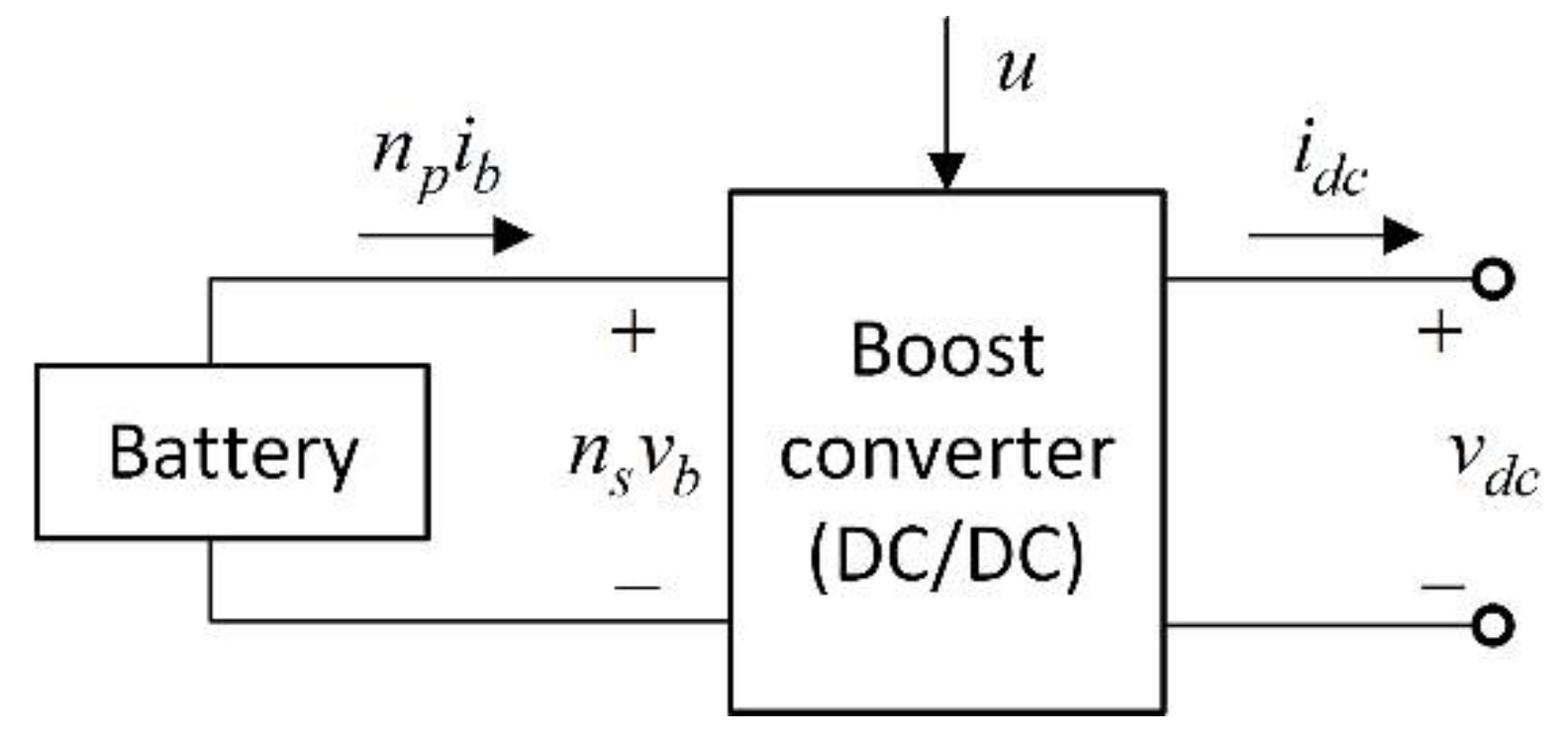
A DC/DC converter (boost converter) is used in the connection between the battery and the Voltage Source Converter (VSC). The battery connection to the VSC is represented by Equations (7) and (8) [16,23]:
where u is the duty cycle of the boost converter; np and ns are the number of parallel and series connected battery cells, respectively; and vdc and idc are the voltage and output current of the boost converter, respectively. More details about these equations can be found in [16]. Figure 4 shows the scheme of association between the battery and the boost converter [23].
According to [23], the voltage vdc is obtained from the current idc and connection capacitor Cdc, through (9):
From Equations (1) and (2), two transfer functions are obtained, as shown in Figure 5.
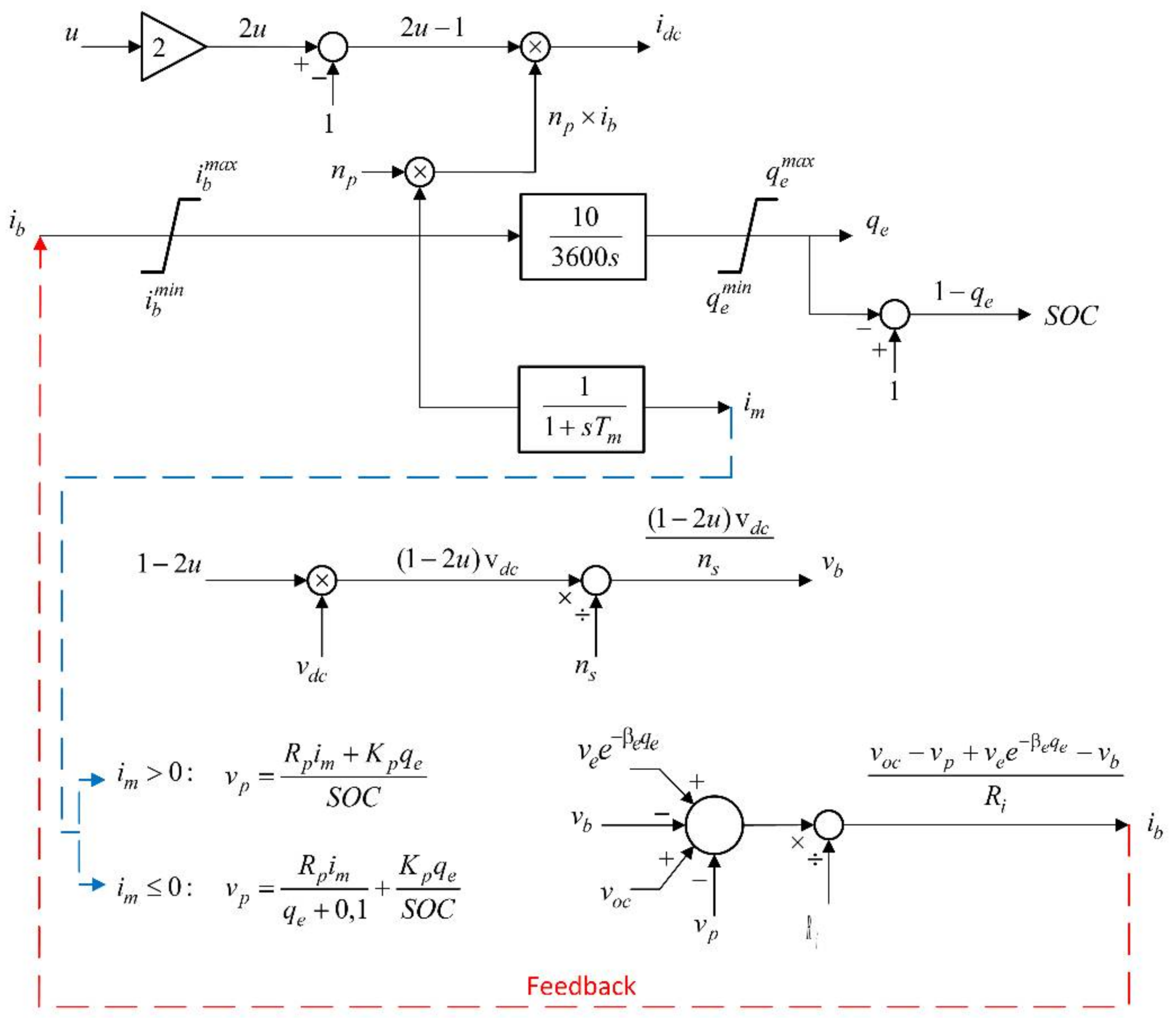
Isolating ib in (3) yields (10), for the calculation of the battery current:
Equations (4) and (5) are used to calculate the polarization voltage, which depends on the current im. If im is greater than zero, (4) is used, otherwise (5) is used. The calculation of the battery state of charge is obtained from (6). From (8) is possible to calculate the output current of the boost converter (idc).
Isolating vb in (7), we have (11), used to calculate the battery voltage:
Figure 6 shows the subsystem of the battery block.
2.1.3. Voltage Source Converter Control Block
Figure 7 shows the subsystem of the voltage source converter control block (adapted from [16]). The design of the controller was realized following classical control methods.
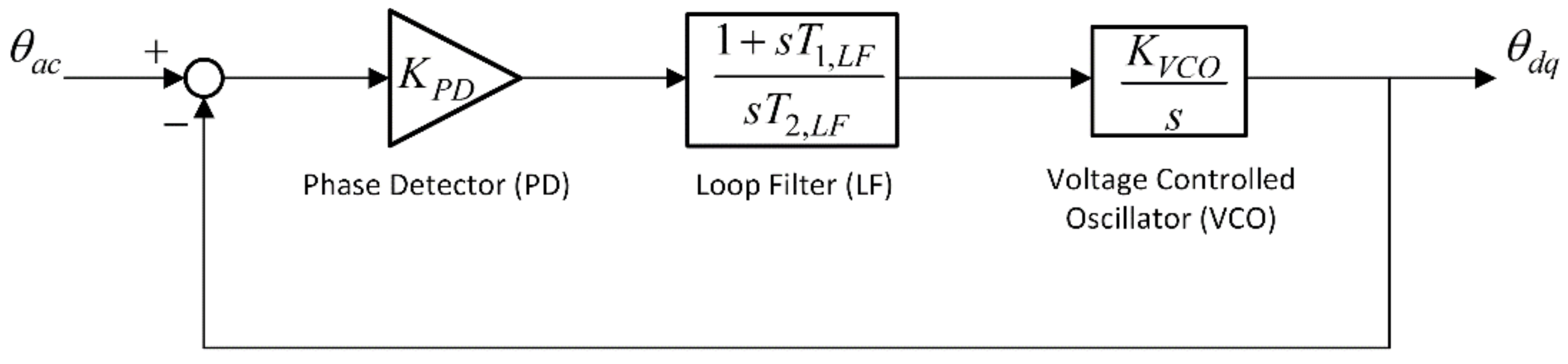
To design suitable controllers, the quantities in alternating current (AC) are expressed using a dq reference axis. This axis rotates with the same speed as the grid voltage phasor . In practice, this is possible through a Phase-Locked Loop (PLL), which is a control system that forces the angle of the axis dq (θdq) to track the angle of the grid voltage (θac) [16].
The PLL block, inside the voltage source converter control block, is shown in detail in Figure 8 [16].
From (12), we have the expressions for vacd and vacq:
2.1.4. Voltage Source Converter Block
Figure 9 shows the subsystem of voltage source converter block (adapted from [16]). In Figure 9, the gain (−1/Cdc) and the integrator (1/s), for the calculation of voltage vdc from the current idc, are described using (9). The open circuit voltage of the capacitor (voc) is an initial condition of the integrator and represents the open circuit voltage of the capacitor Cdc.
3. Test System for a Case Study
The model of the EPS studied in this work (adapted from [24]) is an 11-bus test system with two operating areas, consisting of four generating units, being three conventional generators composed of steam thermal turbines and one wind farm modeled with an equivalent generator representing 600 wind turbines of 1.5 MW. The wind turbine-generator uses the Type-3 doubly-fed asynchronous generator (DFAG) model. In the DFAG technology, a wind turbine can operate at variable speed and respond to a time-varying wind profile as input. The model also considers the physical limits of the machine, considering the lower and upper limits of pitch angle, power injection and rates of change. Power-electronics interfaces that contain power transfer of DFAGs can be modeled as a controlled current injection to the grid [25]. The references [25,26,27] give further details on wind turbine modeling. The wind farm operates at Maximum Power Point Tracking (MPPT) and does not contribute to the frequency control keeping a constant generation (700 MW) throughout the simulation. Tests will be made with BESS connected to the generation buses equipped with substations (1, 2, 3 and 4) and to bus 8. The power flow between areas was set equal to zero, not exciting inter-area oscillations and the inertia of G1 was decreased to create a low-inertia area. The single-line diagram of the test system is shown in Figure 10, and all the parameters are presented in Appendix A. A linear version of this system was obtained using the linmod function form MATLAB/Simulink.
Figure 11 shows the test system represented in block diagrams, implemented in MATLAB/Simulink. The reference voltages (Vref) are calculated through a load flow and are used as initial conditions of the dynamic simulation.
4. Methodology
The task of selecting the most effective point of connection for a BESS to improve the frequency response of EPS is not trivial. Variables such as frequency sag at the first oscillation (frequency nadir) are strongly related to system transient response, resulting in the need for intensive use of time-domain simulations. In this work, it is proposed to use a small-signal stability analysis, obtained with the linearization of the test system model implemented in MATLAB/Simulink, to identify the best connection buses for a selected number of BESSs. Specifically, controllability analysis using eigenvalues are carried out. The proposed approach can be executed as a computer algorithm and may help to identify the best point of connection from a BESS. Subsequently, optional nonlinear simulations may be performed to validate the small-signal analysis.
4.1. Preliminary
From the perspective of the Independent System Operator (ISO), the main goal is to improve the power system frequency. However, this is a challenge because there is not a unique power system frequency. The frequency variation will depend on the bus location, and the devices connected close to them. One potential alternative to analyzing the power system frequency, using linear models, is identifying the frequency regulation mode. In [15], the authors showed how to identify the frequency regulation mode changing droop gain (R) of the governors. In this work, we apply the same procedure changing the droop gain and verifying what modes are the most affected by these changes. Afterward, we analyze the controllability of the frequency regulation mode selected to identify the most effective point of connection for a BESS based on controllability indexes. The controllability is measured from input signals of the mechanical torque of thermal turbines (Tm) and of the mechanical torque of the wind turbine (Tm_wind).
4.2. Proposed Approach
Initially, the system conditions must be checked to verify the candidate buses and the number of BESS devices that will be installed. The candidate buses are selected based on infrastructure capacity such as a high-voltage substation, and the investment capacity of the utility defines the number of BESS devices. The proposed approach is divided into two main steps: identifying the frequency regulation mode and geometric measures analysis (controllability). These two steps are repeated until the number of BESSs is distributed along the system. In the following sections, these two main steps are described in details.
4.2.1. Step (I): Identification of Frequency Regulation Modes and Selection of Interest Mode
This first step is based on the study with frequency regulation modes proposed in [15]. A study was made changing the droop constant (Rp), to vary the droop gain (1/Rp), in the primary frequency control loop of the synchronous generators. Considering the linear representation of the Electrical Power System, described by (15) and (16):
where x is the state vector (vector n); y is the output vector (vector m); u is the control vector (vector r); A is the state matrix (matrix n × n); B is the control matrix (matrix n × r); and C is the output matrix (matrix m × n). From the linear system, the droop of generators is changed aiming to identify the groups of eigenvalues that are mostly affected by this perturbation.
Figure 12 shows the groups of eigenvalues (electromechanical modes) that are most affected by the changes in the droop. The eigenvalues are identified and analyzed in the next step.
In Figure 12, point B refers to eigenvalues with the original value of the droop gain. Point A refers to the corresponding eigenvalues with a decrease of droop value, and point C refers to corresponding eigenvalues with an increase of droop value.
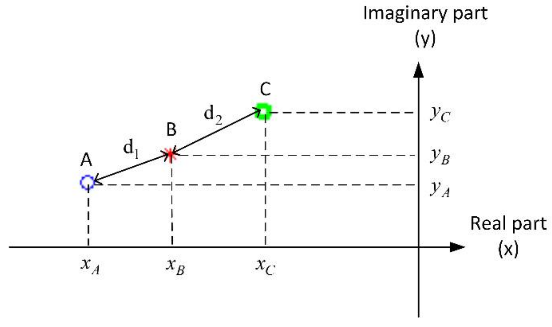
In addition to the study proposed in [15], it is possible to calculate the distances of the eigenvalues obtained for the linearized EPS with the variation of the constant Rp in relation to the eigenvalues for the original linearized system droop values (Rp). Figure 13 shows how to calculate the distances between the eigenvalues in each group.
The distances d1 and d2 are calculated according to Equations (17) and (18):
The eigenvalue group with the largest distance is selected, considering d1 and d2. The eigenvalues of point B (with the original droop values) of the identified group represent the frequency regulation mode selected for step (II).
4.2.2. Step (II): Controllability Analysis of Selected Mode
For the eigenvalues of the frequency regulation mode selected in step (I), controllability is verified through an algorithm based on geometric measurements. This algorithm, proposed by [28,29], is described below. Considering the matrix A from Equation (16), with n distinct eigenvalues (λk, k = 1, ..., n) and matrices corresponding to the left and right eigenvalues, given by Ψ and T. The geometric measures of controllability (mci) associated to the mode k is given by (19) [28,29]:
with bi being the i-th column of the input matrix B (corresponding to the i-th input) and cj the j-th line of the output matrix C (corresponding to the jth output); α(Ψk, bi) is the geometric angle between the input vector i and the kth eigenvector on the left. Geometrically, controllability can be interpreted as the cosine of the angle between the vectors and Ψk. If the cosine of this angle is close to zero, and Ψk are practically orthogonal, indicating a low controllability index of the mode analyzed. Therefore, the greater the angular aperture between the vectors, the better the controllability of the oscillation mode analyzed. The algorithm aims to indicate how much the nth mode of the system is controlled from the outputs and inputs specified in the EPS [28,29]. For the selected mode, the generating unit (synchronous generator or the wind farm) associated with the input signal with the highest controllability index is verified, and the analysis indicates that BESS can be more effective in reducing frequency sag at the first oscillation (frequency nadir) when connected to the bus of this generator.
4.3. Algorithm
The following algorithm can summarize the proposed approach:
- Obtain the power system linear model;
- Check to if there is already BESS devices installed in the system. The bus with a BESS device already installed is not considered as a candidate bus;
- Select a set of candidate buses (Bc) and the maximum number of BESS devices (n = 1, 2,…, nd) that will be installed;
- while n ≤ nd
- Variate the droop of generators and BESS (if it is already in the system);
- Select the oscillation mode with the maximum variation (frequency regulation mode);
- Estimate the controllability using geometric measures;
- The BESS must be installed on the bus with the maximum controllability;
- Remove the selected bus from the set from candidate buses and decrease the number of BESS devices;
- end
- Time domain nonlinear simulation is validating the results (optional).
5. Application Results
This section presents some application results with the BESS model, using the battery allocation methodology described in Section 4. Studies will be realized to identify the best buses for the allocation of two BESS in the test system.
5.1. Allocation of the First BESS
5.1.1. Step (I): Identification of Frequency Regulation Modes and Selection of Interest Mode
Figure 14 shows the electromechanical eigenvalues with a variation of the droop gain (1/Rp).
For each eigenvalue group highlighted in Figure 14, the distances relative to the eigenvalues with the original droop (1/Rp = 232.5582) were calculated using (18) and (19).
Table 1 shows the results for the calculation of the distances between eigenvalues, for each eigenvalue group with changes in the droop.
According to Table 1, the eigenvalues of group 5 presented the largest distance (0.3892), which occurred between points (A) and (B). Therefore, the eigenvalues of this group with the original droop value (−2.5460 ± j0.7549) represent the frequency regulation mode selected for controllability analysis, which will be done in step (II).
5.1.2. Step (II): Controllability Analysis of Selected Mode
Table 2 shows the controllability analysis for the eigenvalues of the mode selected in step (I).
Table 2 shows that the mechanical torque of the thermal turbines (Tm) associated with generator 1 (G1) has the highest controllability index (0.000402). Then, the G1 bus presents the largest controllability, and the analysis indicates that the BESS can be more efficient in the reduction of frequency nadir when connected to the bus of this generator.
5.1.3. Validation of Results through Nonlinear Simulations
For the analysis of nonlinear simulations of EPS using Simulink, the following disturbances cases were applied in the system:
- (a)
- Case 1: Addition of 200 MW in load bus 7, at the instant of 1 s;
- (b)
- Case 2: Addition of 200 MW in load bus 9, at the instant of 1 s.
In the identification of the best bus for the connection of the first BESS in the system, the frequency of Center of Intertia (COI) and average frequency are verified. It is possible to extract the frequency of the COI of the system (fCOI) from (20) [30,31], from the measured frequencies of generators and its inertia constants (synchronous and wind farm):
where N is the number of generation units (synchronous machines and wind farm) in the system, Hi and fi are, respectively, the inertia and the frequency of each generation unit.
- (a)
- Case 1: Addition of 200 MW in load bus 7, at the instant of 1 s
Figure 15 shows the behavior of the frequency of COI and average frequency in the first instants after the application of the disturbance, for tests with one battery in the EPS.
In Figure 15 the frequency of COI and average frequency show that the smallest frequency sag in the first oscillation occurs with the battery connected to the bus 1. Therefore, the best bus for the connection of the first BESS in the system is the bus 1.
- (b)
- Case 2: Addition of 200 MW in load bus 9, at the instant of 1 s
Figure 16 shows the behavior of the frequency of COI and average frequency in the first instants after the application of the disturbance, for tests with one battery in the EPS.
In Figure 16a the frequency of COI show that the smallest frequency nadir occurs with the battery connected to the bus 1 or 2. In Figure 16b the average frequency indicated that the smallest frequency nadir occurs with the battery connected to the bus 8. In this case, therefore, we have different results for the allocation of the first BESS in the system.
5.2. Allocation of the Second BESS
In the study for the allocation of the first BESS in the system, the controllability analysis indicated that the best bus for the battery connection is in the bus of generator 1. Thus, in the analysis for the allocation of the second BESS will be considered the system with one battery allocated at bus 1.
5.2.1. Step (I): Identification of Frequency Regulation Modes and Selection of Interest Mode
Figure 17 shows the electromechanical eigenvalues, with a variation of the droop gain (1/Rp).
For each eigenvalue group highlighted in Figure 17, the distances relative to the eigenvalues with the original droop (1/Rp = 232.5582) were calculated using Equations (18) and (19). Table 3 shows the results for the calculation of the distances between eigenvalues, for each eigenvalue group with changes in the droop.
According to Table 3, the eigenvalues of group 5 presented the largest distance (0.4283), which occurred between points (B) and (C). Therefore, the eigenvalues of this group with the original droop value (−2.2147 ± j0.5018) represent the frequency regulation mode selected for controllability analysis, which will be done in step (II).
5.2.2. Step (II): Controllability Analysis of Selected Mode
Table 4 shows the controllability and analysis for the eigenvalues of the mode selected in step (I).
Table 4 shows that the mechanical torque of the wind turbine (Tm_wind) has the highest controllability index (0.000638), so the wind farm is the most controllable and the analysis indicates that the BESS can be more efficient in the reduction of frequency nadir when connected to the bus of this generation unit.
5.2.3. Validation of Results through Nonlinear Simulations
For the analysis of nonlinear simulations of EPS using Simulink, the same disturbances cases 1 and two applied for the allocation of the first BESS in the system were applied here. In the identification of the best bus for the connection of the second BESS in the system, the frequency of COI and average frequency are verified.
- (a)
- Case 1: Addition of 200 MW in load bus 7, at the instant of 1 s
Figure 18 shows the behavior of the frequency of COI and average frequency in the first instants after the application of the disturbance, for tests with two batteries in the EPS.
In Figure 18a, the frequency of COI indicated that all tests showed similar results for frequency sag in the first oscillation. However, in Figure 18b, the average frequency shows that lowest frequency nadir occurs when the BESS are connected to the buses 1 and 3 or the buses 1 and 4. In this case, the difference among the tests is very small because with two BESS connected in the system the assistance of the batteries in the reduction of frequency nadir is closed to the saturation.
- (b)
- Case 2: Addition of 200 MW in load bus 9, at the instant of 1 s
Figure 19 shows the behavior of the frequency of COI and average frequency in the first instants after the application of the disturbance, for tests with two batteries in the EPS.
In Figure 19, the frequency of COI and average frequency shown that the nadir from BESS in bus 4 is similar to the bus 3. This difference is not significant showing the approach can help to identify the best point of connection.
6. Conclusions
In this work, the application of a generic BESS model was analyzed in a test system with the participation of wind generation to verify the performance of the storage device in the assistance of inertial response and frequency control in energy systems. The main contribution of the paper is a systematic procedure to identify the best point of connection for a BESS based on the controllability of frequency regulation mode, through small-signal stability analysis steps. The controllability analysis with eigenvalues indicated that the best bus for the connection of one BESS in the system is bus 1 and, for the connection of two BESSs in the system, the best points of connection are buses 1 and 4. The nonlinear simulations showed coherence for most the results of the frequency nadir analysis, regarding the controllability analysis with eigenvalues for the BESS point of connection. Some suggestions for future work are: explore other store technologies such as hybrid systems (combining BESS with other technologies) and new control schemes and methods to coordinate control of all these different devices.
Acknowledgments
This work was financially supported by FAPESP under grants no. 2015/18806-7 and 2016/08645-9.
Author Contributions
This paper is the main result of the master dissertation work of Thiago Pieroni, under guidance provided by Daniel Dotta.
Conflicts of Interest
The authors declare no conflict of interest.
Appendix A
This appendix contains tables with model design parameters/constants and initial conditions.

Table A1.
System parameters.
| Grid | AVR | PSS |
|---|---|---|
| Sbase = 100 MVA f0 = 60 Hz Trigger = 1 | Vref (p.u.): G1 = 1.063 G2 = 1.047 G3 = 1.0393 Tr (s) = 0.01 Ta (s) = 1 Tb (s) = 2 Ka (p.u.): G1 = 50 G2 = 50 G3 = 200 | Ks (p.u.) = 20 Tw (s) = 10 T1 (s) = 0.05 T2 (s) = 0.02 T3 (s) = 3 T4 (s) = 5.4 |
Table A2.
Synchronous generators and Wind Farm.
| Synchronous Generators | Wind Farm |
|---|---|
| Tm0 (p.u.): G1 = 7.0001 | wind speed—vw (m/s) = 14 |
| G2 = 7.0001 | Inertia constant—Ht (s) = 4.33 |
| G3 = 7.0053 | Inertia constant—Hg (s) = 0.62 |
| Steam Turbine: | Impedances: |
| Constant droop—Rp (p.u.) = 0.0043 | Ra_wind (p.u.) = 0 |
| tg (s) = 0.2 | Lpp_wind (p.u.) = 0.8 |
| Fhp (s) = 0.3 | - |
| Tch (s) = 0.3 | |
| Trh (s) = 7.0 |
Table A3.
Synchronous generators—bus parameters.
| Bus Number | Voltage (p.u.) | θ (degrees) | Active Power (P) (p.u.) | Reactive Power (Q) (p.u.) | Pload (p.u.) | Qload (p.u.) | Qshunt (p.u.) | Bus Type (1-Vθ, 2-PV, 3-PQ) |
|---|---|---|---|---|---|---|---|---|
| 1 | 1.03 | −6.8313 | 7 | 1.288 | 0 | 0 | 0 | 2 |
| 2 | 1.01 | −16.4508 | 7 | 0.9917 | 0 | 0 | 0 | 2 |
| 3 | 1.03 | −6.8 | 7.0051 | 1.2899 | 0 | 0 | 0 | 1 |
| 4 | 1.01 | −16.432 | 7 | 0.9935 | 0 | 0 | 0 | 2 |
| 5 | 1.0155 | −13.2352 | 0 | 0 | 0 | 0 | 0 | 3 |
| 6 | 1.0003 | −23.0815 | 0 | 0 | 0 | 0 | 0 | 3 |
| 7 | 1.0009 | −31.0777 | 0 | 0 | 13.69 | 1 | 3 | 3 |
| 8 | 1.0116 | −31.1313 | 0 | 0 | 0 | 0 | 0 | 3 |
| 9 | 1.0009 | −31.0623 | 0 | 0 | 13.69 | 1 | 3 | 3 |
| 10 | 1.0003 | −23.0628 | 0 | 0 | 0 | 0 | 0 | 3 |
| 11 | 1.0155 | −13.2087 | 0 | 0 | 0 | 0 | 0 | 3 |
Table A4.
Synchronous generators—line parameters.
| Line from | Line to | R (p.u.) | X (p.u.) | Bshunt (p.u.) | Tap |
|---|---|---|---|---|---|
| 1 | 5 | 0 | 0.0167 | 0 | 1 |
| 2 | 6 | 0 | 0.0167 | 0 | 1 |
| 3 | 11 | 0 | 0.0167 | 0 | 1 |
| 4 | 10 | 0 | 0.0167 | 0 | 1 |
| 5 | 6 | 0.0025 | 0.025 | 0.04375 | 0 |
| 6 | 7 | 0.001 | 0.01 | 0.0175 | 0 |
| 7 | 8 | 0.011 | 0.11 | 0.1925 | 0 |
| 7 | 8 | 0.011 | 0.11 | 0.1925 | 0 |
| 8 | 9 | 0.011 | 0.11 | 0.1925 | 0 |
| 8 | 9 | 0.011 | 0.11 | 0.1925 | 0 |
| 9 | 10 | 0.001 | 0.01 | 0.0175 | 0 |
| 10 | 11 | 0.0025 | 0.025 | 0.04375 | 0 |
Table A5.
Synchronous generators—machine parameters.
| Parameter | Value |
|---|---|
| Rated apparent power (MVA) | 900 |
| Leakage reactance—xl (p.u.) | 0.2 |
| Armature resistante—Ra (p.u.) | 0.000025 |
| d-axis synchronous reactance—xd (p.u.) | 1.8 |
| d-axis transient reactance—x’d (p.u.) | 0.3 |
| d-axis subtransient reactance—x”d (pu) | 0.25 |
| d-axis open-circuit time constant—T’do (s) | 8 |
| d-axis open-circuit subtransient time constant—T”do (s) | 0.03 |
| q-axis sychronous reactance—x_q (pu) | 1.7 |
| q-axis transient reactance—x’_q (pu) | 0.55 |
| q-axis subtransient reactance—x”_q (pu) | 0.25 |
| q-axis open-circuit time constant—T’_qo (s) | 0.4 |
| q-axis open circuit subtransient time constant—T”_qo (s) | 0.05 |
| inertia constant—H (s) | G1 = 4.5 |
| G2 = 6.5 | |
| G3 = 6.175 | |
| damping coefficient—D (pu) | 0 |
References
- Chassin, D.P.; Huang, Z.; Donnelly, M.K.; Hassler, C.; Ramirez, E.; Ray, C. Estimation of WECC System Inertia Using Observed Frequency Transients. IEEE Trans. Power Syst. 2005, 20, 1190–1192. [Google Scholar] [CrossRef]
- Jimenez, J.D.L.; Ramırez, J.M.; David, F.M. Allocation of PMUs for power system-wide inertial frequency response estimation. The Institution of Engineering and Technology. IET Gener. Transm. Distrib. 2017, 11, 2902–2911. [Google Scholar] [CrossRef]
- European Network of Transmission System Operators for Electricity (ENTSO-E). Future System Inertia. Available online: https://www.entsoe.eu/Documents/Publications/SOC/Nordic/Nordic_report_Future_System_Inertia.pdf (accessed on 25 January 2018).
- Lugnani, L.; Dotta, D.; Ferreira, J.M.F.; Decker, I.C.; Chow, J.H. Frequency Response Estimation Following Large Disturbances using synchrophasors. IEEE Power Energy Soc. Gen. Meet. 2018, in press. [Google Scholar]
- Koller, M.; Borsche, T.; Ulbig, A.; Andersson, G. Review of grid applications with the Zurich 1 MW battery energy storage system. Electr. Power Syst. Res. 2015, 120, 28–135. [Google Scholar] [CrossRef]
- Schmutz, J. Primary Frequency Control Provided by Battery; EEH—Power Systems Laboratory, ETH Zürich: Zurich, Switzerland, 2013. [Google Scholar]
- Hollinger, R.; Diazgranados, L.M.; Wittwer, C.; Engel, B. Optimal Provision of Primary Frequency Control with Battery Systems by Exploiting all Degrees of Freedom within Regulation. Energy Procedia 2016, 99, 204–214. [Google Scholar] [CrossRef]
- Mégel, O.; Mathieu, J.L.; Andersson, G. Maximizing the Potential of Energy Storage to Provide Fast Frequency Control. In Proceedings of the 4th IEEE PES Innovative Smart Grid Technologies Europe (ISGT EUROPE), Copenhagen, Denmark, 6–9 October 2013. [Google Scholar]
- Kalyani, S.; Nagalakshmi, S.; Marisha, R. Load Frequency Control Using Battery Energy Storage System in Interconnected Power System. In Proceedings of the 2012 Third International Conference on Computing, Communication and Networking Technologies (ICCCNT), Coimbatore, India, 26–28 July 2012. [Google Scholar]
- Sen, U.; Kumar, N. Load Frequency Control with Battery Energy Storage System. In Proceedings of the 2014 International Conference on Power, Control and Embedded Systems (ICPCES), Allahabad, India, 26–28 December 2014. [Google Scholar]
- Chowdary, K.R.; Santhoshi, P.; Bhaskararao, S.; Anusha, T.; Devarao, S.V. Load Frequency Control of A Typical Two Area Interconnected Power System by Using Battery Energy Storage System. Int. J. Eng. Res. Appl. 2014, 4, 145–150. [Google Scholar]
- Mercier, P.; Cherkaoui, R.; Oudalov, A. Optimizing a Battery Energy Storage System for Frequency Control Application in an Isolated Power System. IEEE Trans. Power Syst. 2009, 24, 1469–1477. [Google Scholar] [CrossRef]
- Toge, M.; Kurita, Y.; Iwamoto, S. Supplementary Load Frequency Control with Storage Battery Operation Considering SOC under Large-scale Wind Power Penetration. In Proceedings of the IEEE Power & Energy Society General Meeting, Vancouver, BC, Canada, 21–25 July 2013. [Google Scholar]
- Zhu, D.; Hug-Glanzmann, G. Coordination of storage and generation in power system frequency control using an H∞ approach. IET Gener. Transm. Distrib. 2013, 7, 1263–1271. [Google Scholar] [CrossRef]
- Wilches-Bernal, F.; Chow, H.; Sanchez-Gasca, J.J. A Fundamental Study of Applying Wind Turbines for Power System Frequency Control. IEEE Trans. Power Syst. 2016, 31, 1496–1505. [Google Scholar] [CrossRef]
- Ortega, A.; Milano, F. Generalized Model of VSC-Based Energy Storage Systems for Transient Stability Analysis. IEEE Trans. Power Syst. 2016, 31, 3369–3380. [Google Scholar] [CrossRef]
- Gatta, F.M. Application of a LiFePO4 Battery Energy Storage System to Primary Frequency Control: Simulations and Experimental Results. Energies 2016, 9, 887. [Google Scholar] [CrossRef]
- Knap, V.; Chaudhary, S.K.; Store, D.-I.; Swierczynski, M.; Craciun, B.-I.; Teodorescu, R. Sizing of an Energy Storage System for Grid Inertial Response and Primary Frequency Reserve. IEEE Trans. Power Syst. 2016, 31, 3447–3456. [Google Scholar] [CrossRef]
- Arita, M.; Yokoyama, A.; Tada, Y. Evaluation of Battery System for Frequency Control in Interconnected Power System with a Large Penetration of Wind Power Generation. In Proceedings of the International Conference on Power System Technology, Chongqing, China, 22–26 October 2006; pp. 1–7. [Google Scholar]
- Benini, M.; Canavese, S.; Cirio, D.; Gatti, A. Battery Energy Storage Systems for the Provision of Primary and Secondary Frequency Regulation in Italy. In Proceedings of the 2016 IEEE 16th International Conference on Environment and Electrical Engineering (EEEIC), Florence, Italy, 6–8 June 2016. [Google Scholar]
- Shankar, R.; Chatterjee, K.; Bhushan, R. Impact of energy storage system on load frequency control for diverse sources of the interconnected power system in deregulated power environment. Electr. Power Energy Syst. 2016, 79, 11–26. [Google Scholar] [CrossRef]
- Kerdphol, T.; Qudaih, Y.; Mitani, Y. Optimum battery energy storage system using PSO considering dynamic demand response for microgrids. Electr. Power Energy Syst. 2016, 83, 58–66. [Google Scholar] [CrossRef]
- Ortega, A.; Milano, F. Design of a Control Limiter to Improve the Dynamic Response of Energy Storage Systems. In Proceedings of the IEEE Power & Energy Society General Meeting, Denver, CO, USA, 26–30 July 2015; pp. 1–5. [Google Scholar]
- Kundur, P. Power System Stability, and Control; EPRI Power System Engineering Series; McGraw-Hill, Inc.: Riverside, CA, USA, 1994. [Google Scholar]
- Wilches-Bernal, F. Applications of Wind Generation for Power System Frequency Control, Inter-Area Oscillations Damping and Parameter Identification. Ph.D. Thesis, Rensselaer Polytechnic Institute, Troy, NY, USA, 2015. [Google Scholar]
- Motta, R.T.; Dotta, D. Representação Computacional de Parques Eólicos: Comparativo entre Modelos de Primeira e Segunda Geração; XXIV Seminário Nacional de Produção e Transmissão de Energia Elétrica—SNPTEE: Curitiba, Brazil, 2017. (In Portuguese) [Google Scholar]
- Clark, K.; Miller, N.W.; Sanchez-Gasca, J.J. Modeling of GE Wind Turbine-Generators for Grid Studies; GE Energy: Boston, MA, USA, 2009. [Google Scholar]
- Dotta, D. Controle Hierárquico Usando Sinais de Medição Fasorial Sincronizada. Ph.D. Thesis, Universidade Federal de Santa Catarina, Florianópolis, Brazil, 2009. (In Portuguese). [Google Scholar]
- Heniche, A.; Kamwa, I. Control loops selection to damp inter-area oscillations of electrical networks. IEEE Trans. Power Syst. 2002, 17, 378–384. [Google Scholar] [CrossRef]
- Júnior, S.S.D.S. Proposta e Avaliação de um Método Adaptativo de Corte de Carga. Master’s Thesis, UFRJ/COPPE, Rio de Janeiro, Brazil, 2017. (In Portuguese). [Google Scholar]
- Rudez, U.; Mihalic, R. Analysis of Underfrequency Load Shedding Using a Frequency Gradient. IEEE Trans. Power Deliv. 2011, 26, 565–575. [Google Scholar] [CrossRef]
Figure 1.
Scheme of BESS connected to the grid (adapted from [16]).
Figure 1.
Scheme of BESS connected to the grid (adapted from [16]).

Figure 2.
BESS modeling organized in block diagrams.

Figure 3.
Battery control block.

Figure 4.
Scheme of association between the battery and the boost converter [23].
Figure 4.
Scheme of association between the battery and the boost converter [23].

Figure 5.
(a) Transfer function relative to Equation (1); (b) Transfer function relative to Equation (2).
Figure 5.
(a) Transfer function relative to Equation (1); (b) Transfer function relative to Equation (2).

Figure 6.
Battery block.

Figure 7.
Voltage source converter control block.

Figure 8.
PLL block, inside the voltage source converter control block [16].
Figure 8.
PLL block, inside the voltage source converter control block [16].

Figure 9.
Voltage source converter block.

Figure 10.
Single-line diagram representation of the 11-bus test system (adapted from [24]).
Figure 10.
Single-line diagram representation of the 11-bus test system (adapted from [24]).

Figure 11.
Test system represented in block diagrams, implemented in MATLAB/Simulink.

Figure 12.
Identification of the groups of electromechanical eigenvalues with a real part in the interval that is most affected by the changes in the droop.
Figure 12.
Identification of the groups of electromechanical eigenvalues with a real part in the interval that is most affected by the changes in the droop.

Figure 13.
Distances between eigenvalues.

Figure 14.
Electromechanical eigenvalues with the highlight for the groups that are most affected by the changes in the droop.
Figure 14.
Electromechanical eigenvalues with the highlight for the groups that are most affected by the changes in the droop.

Figure 15.
(a) Frequency of COI; (b) Average frequency.

Figure 16.
(a) Frequency of COI; (b) Average frequency.

Figure 17.
Eigenvalues with a real part in the interval (−3, 0), with the highlight for the groups that are most affected by the changes in the droop.
Figure 17.
Eigenvalues with a real part in the interval (−3, 0), with the highlight for the groups that are most affected by the changes in the droop.

Figure 18.
(a) Frequency of COI; (b) Average frequency.

Figure 19.
(a) Frequency of COI; (b) Average frequency.

Table 1.
Electromechanical Eigenvalues that are most affected by the changes in the droop.
| Eigenvalue Group | Droop (1/Rp) = 100 (A) | Droop (1/Rp) = 232.5582 (B) | Droop (1/Rp) = 500 (C) | Distance between | ||||
|---|---|---|---|---|---|---|---|---|
| (A) and (B) | (B) and (C) | |||||||
| Real | Imag | Real | Imag | Real | Imag | Module | Module | |
| 1 | −0.5654 | ±7.9441 | −0.5320 | ±7.9771 | −0.4665 | ±8.0426 | 0.0469 | 0.0927 |
| 2 | −0.2443 | ±4.8949 | −0.2176 | ±4.9696 | −0.1630 | ±5.1121 | 0.0794 | 0.1526 |
| 3 | −2.3124 | ±2.1027 | −2.2860 | ±2.1793 | −2.2202 | ±2.2582 | 0.0810 | 0.1027 |
| 4 | −1.2941 | ±2.0030 | −1.1496 | ±2.1534 | −0.9527 | ±2.4835 | 0.2086 | 0.3843 |
| 5 | −2.6521 | ±0.3805 | −2.5460 | ±0.7549 | −2.4839 | ±1.0121 | 0.3892 | 0.2646 |
Table 2.
Controllability analysis of the eigenvalues of the mode selected in step (I).
| Eigenvalues −2.5460 ± j0.7549 Controllability | |
|---|---|
| Input Signals | Index |
| Tm(1) | 0.000402 |
| Tm(2) | 0.000390 |
| Tm(3) | 0.000321 |
| Tm_wind | 0.000246 |
Table 3.
Eigenvalues with a real part in the interval (−3, 0) that are most affected by the changes in the droop.
Table 3.
Eigenvalues with a real part in the interval (−3, 0) that are most affected by the changes in the droop.
| Eigenvalue Group | Droop (1/Rp) = 100 (A) | Droop (1/Rp) = 232.5582 (B) | Droop (1/Rp) = 500 (C) | Distance between | ||||
|---|---|---|---|---|---|---|---|---|
| (A) and (B) | (B) and (C) | |||||||
| Real | Imag | Real | Imag | Real | Imag | Module | Module | |
| 1 | −1.1690 | ±8.0667 | −1.1316 | ±8.1030 | −1.0584 | ±8.1749 | 0.0521 | 0.1026 |
| 2 | −0.5319 | ±4.9883 | −0.4975 | ±5.0667 | −0.4290 | ±5.2145 | 0.0856 | 0.1629 |
| 3 | −1.7123 | ±2.5085 | −1.6593 | ±2.6669 | −1.4709 | ±2.9954 | 0.1670 | 0.3787 |
| 4 | −2.3277 | ±2.4325 | −2.2285 | ±2.4182 | −2.1466 | ±2.3593 | 0.1002 | 0.1009 |
| 5 | - | - | −2.2147 | ±0.5018 | −2.1862 | ±0.9291 | - | 0.4283 |
| 6 | −1.4790 | ±0.1816 | −1.3885 | 0.0000 | −1.3164 | 0.0000 | 0.2029 | 0.0721 |
Table 4.
Controllability analysis of the eigenvalues of the mode selected in step (I).
| Eigenvalues −2.2147 ± j0.5018 Controllability | |
|---|---|
| Input Signals | Index |
| Tm_wind | 0.000638 |
| Tm(3) | 0.000474 |
| Tm(2) | 0.000307 |
© 2018 by the authors. Licensee MDPI, Basel, Switzerland. This article is an open access article distributed under the terms and conditions of the Creative Commons Attribution (CC BY) license (http://creativecommons.org/licenses/by/4.0/).
Share and Cite
MDPI and ACS Style
Pieroni, T.; Dotta, D. Identification of the Most Effective Point of Connection for Battery Energy Storage Systems Focusing on Power System Frequency Response Improvement. Energies 2018, 11, 763. https://doi.org/10.3390/en11040763
AMA Style
Pieroni T, Dotta D. Identification of the Most Effective Point of Connection for Battery Energy Storage Systems Focusing on Power System Frequency Response Improvement. Energies. 2018; 11(4):763. https://doi.org/10.3390/en11040763
Chicago/Turabian StylePieroni, Thiago, and Daniel Dotta. 2018. "Identification of the Most Effective Point of Connection for Battery Energy Storage Systems Focusing on Power System Frequency Response Improvement" Energies 11, no. 4: 763. https://doi.org/10.3390/en11040763
Note that from the first issue of 2016, this journal uses article numbers instead of page numbers. See further details here.