A Generalised Assessment of Working Fluids and Radial Turbines for Non-Recuperated Subcritical Organic Rankine Cycles

Abstract

The aim of this paper is to conduct a generalised assessment of both optimal working fluids and radial turbine designs for small-scale organic Rankine cycle (ORC) systems across a range of heat-source temperatures. The former has been achieved by coupling a thermodynamic model of subcritical, non-recperated cycles with the Peng–Robinson equation of state, and optimising the working-fluid and cycle parameters for heat-source temperatures ranging between 80 $°\mathrm{C}$ and 360 $°\mathrm{C}$. The critical temperature of the working fluid is found to be an important parameter governing working-fluid selection. Moreover, a linear correlation between heat-source temperature and the optimal critical temperature that achieves maximum power output has been found for heat-source temperatures below 300 $°\mathrm{C}$ ($T_{\mathrm{cr}}=0.830T_{\mathrm{hi}}+41.27$). This correlation has been validated against cycle calculations completed for nine predefined working fluids using both the Peng–Robinson equation of state and using the REFPROP program. Ultimately, this simple correlation can be used to identify working-fluid candidates for a specific heat-source temperature. In the second half of this paper, the effect of the heat-source temperature on the optimal design of a radial-inflow turbine rotor for a 25 kW subcritical ORC system has been studied. As the heat-source temperature increases, the optimal blade-loading coefficient increases, whilst the optimal flow coefficient reduces. Furthermore, passage losses are dominant in turbines intended for low-temperature applications. However, at higher heat-source temperatures, clearance losses become more dominant owing to the reduced blade heights. This information can be used to identify the most direct route to efficiency improvements in these machines. Finally, it is observed that the transition from a conventional converging stator to a converging-diverging stator occurs at heat-source temperatures of approximately 165 $°\mathrm{C}$, whilst radially-fibered turbines seem unsuitable as the heat-source temperature exceeds 250 $°\mathrm{C}$; these conclusions can be used to inform expander design and selection at an early stage.

1. Introduction

In the past decade, organic Rankine cycle (ORC) systems have gained significant traction as a viable technology for the conversion of low-temperature heat (<400 $°\mathrm{C}$) into power [1]. ORC systems are commercially available with power outputs of the order of 100 kW_e and above, but the penetration of the domestic and commercial scales has been elusive owing to technical and economical challenges. As such, there have been a number of research activities focussing on ORC systems of this scale. Arguably, two of the most critical components are the working fluid and the expander. The former defines the potential of the cycle to convert thermal energy into work, whilst an efficient expansion is critical to realise as much of this potential as possible.

The list of possible working fluids is vast, including fluids from the hydrocarbon, hydrofluorocarbon, hydrofluoroolefin and siloxane families. An optimal fluid should result in good thermodynamic and component performance, have good material compatibility, be safe, available and cheap. Moreover, environmental properties are becoming increasingly important, and the selection process must keep up-to-date with changing legislation, such as the recent Kigali agreement [2]. The selection process typically involves considering a group of known fluids, taken from programs such as REFPROP [3] or CoolProp [4], and screening these fluids based on predefined criteria. This is followed by a system optimisation study in which each fluid is considered in turn. Notable examples can be found in Refs. [5,6]. Other examples include those by Drescher and Brüggemann [7], who identified five optimal fluids for a biomass application from an initial group of 1800 substances. More recently, the same group has used computational chemistry to identify fluids for automotive waste-heat recovery applications [8,9], evaluating over 3000 promising candidates from the 72 million substances available in the PubChem database. Vivian et al. [10] optimised four different ORC configurations with 27 working fluids, and produced guidelines for fluid selection based on the heat-source temperature. More specifically, it was suggested that the difference between the heat-source temperature and the critical temperature of the fluid is an important selection criteria.

A more sophisticated approach to working-fluid selection can be achieved using computer-aided molecular design (CAMD). In this approach, group-contribution methods, such as the Joback and Reid method [11], are used to determine key fluid parameters based on the functional groups that make up the molecule. By combining these group-contribution methods with an equation of state, such as a cubic equation of state or the more advanced statistical associating fluid theory (SAFT) [12], and describing the fluid structure using integer variables, the fluid structure can be optimised alongside the thermodynamic cycle. One of the first CAMD-ORC studies was completed by Papadopoulos et al. [13], who considered a range of factors such as performance, cost, toxicity and flammability. Palma-Flores et al. [14] focussed primarily on thermodynamic performance and safety characteristics, whilst Cignitti et al. [15] considered thermodynamic performance alongside the heat exchanger requirements. In comparison to these studies, which all use a cubic equation of state, studies have also been conducted using SAFT. Lampe et al. [16,17] devised a two-stage CAMD-ORC optimisation framework, based on the perturbed-chain SAFT equation of state [18], and determined an optimal fluid for a 120 $°\mathrm{C}$ heat source based on thermodynamic performance. Schilling et al. [19] reduced this to a single-stage optimisation framework, and considered the multi-objective optimisation of an ORC system for a combined-heat and power application, in addition to considering the preliminary design of the turbine. White et al. [20] developed a CAMD-ORC model, based on the SAFT-$\gamma$ Mie equation of state, and applied this model to identify optimal hydrocarbon working fluids for 150, 250 and 350 $°\mathrm{C}$ heat sources.

Compared to REFPROP, CoolProp and SAFT, cubic equations of state are not as accurate. However, since they require less fluid parameters and can be easily implemented within a process model, they remain a viable research tool. Lujàn et al. [21] compared the Peng–Robinson (PR) [22] and the Redlich–Kwong–Soave (RKS) [23] equations of state for modelling the expansion of R245fa within an ORC and found that these equations of state corresponded to deviations in the specific energy of expansion of 6% and 8%, respectively, compared to REFPROP. Brignoli and Brown [24] coupled an ORC thermodynamic model with the PR equation of state. A comparison between the saturation pressures, latent heats of vaporisation, saturation densities and ideal specific-heat capacity terms calculated using PR and using REFPROP found that for the 31 fluids considered, the maximum error was generally below 10%. Su and Deng [25] report similar conclusions. Frutiger et al. [26] compared uncertainty assessments of the RKS and PC-SAFT equations of state, and found that the RKS equation of state could be preferable with regards to minimising uncertainty.

Regarding expander technology for small-scale ORC systems, either volumetric- or turboexpanders can be considered. Examples of volumetric expanders are scroll, screw and reciprocating-piston expanders, which are all characterised by low rotational speeds, simple construction, low part count and low cost. Scroll expanders are generally considered for power outputs in the order of a few kilowatts, whilst screw expanders are considered when the power output is in the order of a few tens of kilowatts up to a few hundred kilowatts. However, due to mechanical design constraints, screw and scroll expanders are limited by their built-in volume ratio, and as such single-stage systems are limited to low-temperature applications, in which the volumetric expansion ratio is typically below 10. Reciprocating-piston expanders can achieve higher volume ratios, but are at an early stage of development [27]. By comparison, turboexpanders can achieve a high expansion ratio over a single stage, which means they are suitable for the full range of heat-source temperatures considered within this paper, and also have advantages with regards to size, compactness and can achieve a high efficiency at the design point. Therefore, the focus of this paper is on turboexpanders for small-scale ORC applications, although turboexpanders correspond to higher rotational speeds than volumetric expanders which can increase cost, and the low speed of sound of organic fluids often leads to supersonic conditions within the turbine. The design of an ORC turbine is achieved by combining a real-gas model with conventional turbomachinery design practices, for example in Refs. [28,29,30]. Lio et al. [31,32] attempted to establish general recommendations for the design of axial [31] and radial [32] turbines, by evaluating the effects of turbine size and expansion ratio on the turbine efficiency. Their results suggest there could be a reduction in turbine efficiency as the operating conditions approach the critical temperature. Advancements in computational power mean turbine design models can be integrated with thermodynamic cycle models, and the integrated optimisation of both the thermodynamic cycle and turbine can be completed, as demonstrated in Refs. [33,34].

In general, the majority of studies within the literature follow a similar approach to fluid selection and turbine design in that a list of candidate fluids is generated and a parametric optimisation study is completed. Whilst these studies can identify the optimal fluid and turbine design for a specific application, they provide little insight into the general characteristics that make a fluid an optimal choice for a particular heat-source temperature, or the effect of the heat-source temperature on the turbine design. Existing CAMD-ORC models facilitate a more generalised approach to fluid selection, but do not provide sufficient detail with regards to component design, and are typically applied to individual case studies. On the other hand, a market assessment of ORC technology, such as the one completed by Landelle et al. [35], are useful to make general observations with regards to component selection and expected performance, but are too general to make recommendations with regards to both working-fluid selection and turbine design.

With this in mind, there are two objectives of this paper; the first is to use principles taken from CAMD, namely the optimisation of fluid parameters such as the critical properties, to identify theoretically optimal fluids for a range of heat-source temperatures. The second objective is to use this information to make a generalised assessment of how the heat-source temperature affects the design and performance of a radial turbine. To the authors’ knowledge, this study is the first to apply these methods within this context, and the results are useful to make more informed choices with regards to both working-fluid selection and turbine design for future applications. Not only will this information be useful to system designers considering a specific application, but a more generalised approach favours a transition towards a more standardised design method, which should enable future improvements in the economy-of-scale and lead to cost reductions in small-scale ORC systems.

Following this introduction, the developed models are described in Section 2, and the optimisation methods are described in Section 3. In Section 4, a case study is defined that considers a range of different heat-source temperatures, and the results from this case study are presented and discussed in Section 5. Finally, the main conclusions from this research are presented in Section 6.

2. Modelling

2.1. Thermodynamic Properties

In line with the motivation behind this research, an equation of state is required that is capable of describing a working fluid in a generalised way, rather than using software such as REFPROP. Cubic equations of state are a suitable choice, and have previously been used within the context of cycle and expander modelling for ORC systems [21,24,25]. Specifically, the Peng–Robinson equation of state is used to model the thermodynamic properties of the working fluid, which is defined as [22]:

$$p=\frac{RT}{V_{\mathrm{m}}-b}-\frac{a\alpha \left(T\right)}{V_{\mathrm{m}}^2+2b{V}_{\mathrm{m}}-b^2},$$

(1)

where p is the pressure in Pa, R is the universal gas constant with units J/(mol K), T is the temperature in K, and $V_{\mathrm{m}}$ is the molar volume with units of ${\mathrm{m}}^3$/mol. The parameters a and b are fluid-specific parameters given by:

$$a={\displaystyle \frac{0.45724R^2{T}_{\mathrm{cr}}^2}{p_{\mathrm{cr}}}},$$

(2)

$$b={\displaystyle \frac{0.0778R{T}_{\mathrm{cr}}}{p_{\mathrm{cr}}}},$$

(3)

where $T_{\mathrm{cr}}$ and $p_{\mathrm{cr}}$ are the temperature and pressure at the critical point. These terms are derived by setting the derivatives of Equation (1), $\partial p/\partial V_{\mathrm{m}}$ and ${\partial }^{2}p/\partial V_{\mathrm{m}}^2$, equal to zero at the critical point. The function $\alpha \left(T\right)$ introduces a temperature dependence to the term on the right-hand side of Equation (1):

$$\alpha \left(T\right)={\left(1+n\left(1-\sqrt{\frac{T}{T_{\mathrm{cr}}}}\right)\right)}^2,$$

(4)

where n is a quadratic function of the acentric factor $\omega$:

$$n=0.37464+1.54225\omega -0.26992{\omega }^2.$$

(5)

The acentric factor is another fluid-specific parameter, defined as $\omega =-{\log }_{10}\left(p_r^{\mathrm{sat}}\right)-1$, where $p_r^{\mathrm{sat}}$ is the reduced saturation pressure at a reduced temperature of 0.7.

Using Equation (1), the fugacity and the departure functions for enthalpy and entropy can be derived. For brevity, these calculations will not be reproduced here, but can be found in Ref. [36]. Using these functions, the saturation pressure $p_{\mathrm{sat}}$ and the latent-heat of vapourisation can be determined. Under saturated conditions, the liquid and vapour fugacity are equal. Therefore, for a defined temperature, the saturation pressure can be found by varying the pressure until this condition is met. Within the model, this procedure is completed using the Newton–Raphson method.

To determine the enthalpy and entropy for a single-phase fluid, the ideal specific-heat capacity $c_{\mathrm{p},\mathrm{id}}$ as a function of temperature is required. This is defined using a second-order polynomial:

$$c_{\mathrm{p},\mathrm{id}}\left(T\right)=A+BT+C{T}^2,$$

(6)

where A, B and C are constants. The enthalpy h in J/mol and the entropy s in J/(mol K) can be calculated from Equations (1) and (6). Further details of these calculations can be found in Ref. [36].

Combining the Peng–Robinson equation of state with a second-order polynomial for $c_{\mathrm{p},\mathrm{id}}$ means a fluid can be fully described by six parameters, namely $T_{\mathrm{cr}}$, $p_{\mathrm{cr}}$, $\omega$, A, B and C. This, in turn, allows a more generalised approach to ORC working-fluid selection by enabling these parameters to become variables during a cycle optimisation process. With this in mind, it is noted that the equation of state is defined in terms of the molar volume and the universal gas constant, which removes the need of defining the molar mass as an additional parameter. Moreover, the Peng–Robinson equation of state is selected over other possible equations of state that contain more adjustable parameters, for example the Peng–Robinson–Stryjek–Vera equation of state [37], since reducing the number of fluid parameters reduces the number of optimisation variables, therefore simplifying the optimisation. It is noted that the validity of the Peng–Robinson equation of state for modelling ORC fluids will be verified later on.

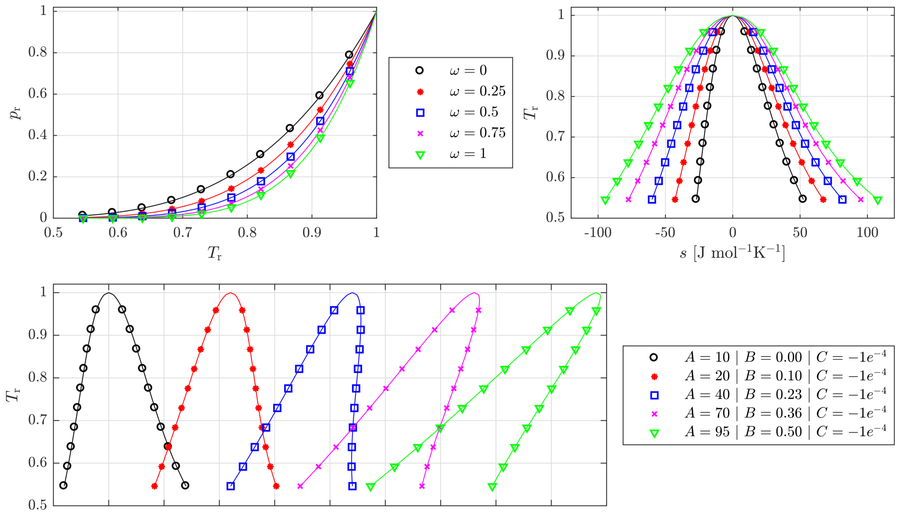
In Figure 1, the effect of the fluid parameters on the saturation curve of a fluid is investigated with $T_{\mathrm{cr}}=500\mathrm{K}$ and $p_{\mathrm{cr}}=30\mathrm{bar}$. As $\omega$ increases towards 1, the same pressure ratio can be obtained over a smaller temperature ratio, suggesting that a high value of $\omega$ is favourable for maximising the pressure ratio for a given heat-source and heat-sink temperature. Moreover, as $\omega$ increases, the latent-heat and entropy of vapourisation both increase, resulting in a widening of the saturation curve on a T–s diagram. Depending on the application, this may be an advantage or a disadvantage. In applications where maximising the cycle efficiency is the objective, a high latent-heat of vapourisation results in a high specific work output [38]. However, in waste-heat recovery applications, where the objective is maximising the power output, a lower latent-heat means allowing a larger proportion of the heat-transfer process within the evaporator to occur in the preheating region, thus resulting in a better thermal match to the heat source, and a higher power output. Finally, the $c_{\mathrm{p},\mathrm{id}}$ polynomial defines whether the saturated-vapour curve has a positive or negative gradient, but plays no role in determining the saturation properties of the fluid.

2.2. ORC Modelling

Within this paper, the Peng–Robinson equation of state will be used to identify the optimal fluid parameters that result in the best thermodynamic performance from a subcritical, non-recuperated ORC intended for a waste-heat recovery application. This type of system is the most common cycle, and has advantages with regards to both simplicity and cost. Other cycles, such as supercritical and cascaded cycles, two-phase expansion, and cycles operating with mixtures may offer performance benefits, but introduce additional complexities or increased costs. For example, supercritical cycles operate under higher pressures, expanders for two-phase expansion are not widely available, whilst fluid mixtures and cascaded cycles typically require much larger heat exchangers. Recuperated cycles can also be considered, but for waste-heat recovery applications, they may have limited effect on improving the thermodynamic performance of the system, as a recuperator could increase the heat-source temperature at the outlet of the evaporator.

A subcritical, non-recuperated Rankine cycle, shown in Figure 2, can be defined by the condensation temperature $T_1$, the evaporation reduced pressure $p_{\mathrm{r}}$ (defined as $p_2/p_{\mathrm{cr}}$, where $p_2$ is the evaporation pressure), and the amount of superheat $\Delta T_{\mathrm{sh}}$. Alongside the pump and turbine efficiencies, denoted ${\eta }_{\mathrm{p}}$ and ${\eta }_{\mathrm{t}}$ respectively, this defines all thermodynamic state points. The working-fluid mass-flow rate ${\dot{m}}_{\mathrm{w}}$ is determined by applying an energy balance to the evaporator:

$${\dot{m}}_{\mathrm{w}}=\frac{{\dot{m}}_{\mathrm{h}}{c}_{\mathrm{p},\mathrm{h}}(T_{\mathrm{hi}}-T_{\mathrm{hp}})}{h_3-h_{2^{\prime }}},$$

(7)

where ${\dot{m}}_{\mathrm{h}}$ and $c_{\mathrm{p},\mathrm{h}}$ are the heat-source mass-flow rate and specific-heat capacity respectively, $T_{\mathrm{hi}}$ is the heat-source temperature, and $T_{\mathrm{hp}}$ is the heat-source temperature at the start of evaporation. This is defined by specifying, as a model input, the temperature difference:

$$\Delta T_{\mathrm{p}}=T_{\mathrm{hp}}-T_{2^{\prime }},$$

(8)

where $T_{2^{\prime }}$ is the saturation temperature of the working fluid at the evaporation pressure.

The cycle analysis is completed by applying an energy balance to the preheating, precooling, and condensation processes to determine the temperature differences between the fluid and the heat-source and heat-sink streams, which must be greater than the minimum allowable temperature differences, denoted ${PP}_{\mathrm{h}}$ and ${PP}_{\mathrm{c}}$ respectively. The temperature differences are calculated along the complete heat-transfer process to ensure the pinch constraints are not violated; during preliminary studies, it was found that, due to the curvature of the isobars, it is possible for the pinch constraint to be satisfied at location 2 and location $2^{\prime }$, but violated at a position between these two locations. In some cases, the pinch point will correspond to the temperature difference at the start of evaporation (i.e., ${PP}_{\mathrm{h}}=\Delta T_{\mathrm{p}}$); however, the pinch point could in fact occur at any location within the preheater, or even at the expander inlet if the degree of superheat is sufficiently high.

Within the cycle model, there is no consideration of the heat-exchanger area requirements. This is because prediction methods for the thermal conductivity, viscosity and surface tensions are required to be able to accurately size the heat exchangers. However, these cannot be calculated using the Peng–Robinson equation or state, and cannot be easily determined without either predefining the working fluid, or using relatively complex group-contribution methods, which, in turn, require the full molecular structure of the working fluid to be defined. This introduces significant complexity to the model, as demonstrated in Ref. [20] in which a relatively complex set of empirical equations are implemented to determine these properties for only hydrocarbon fluids. Moreover, requiring the molecular structure to be defined, does, by definition, lead to a less general approach. For this reason, the authors have chosen to focus on thermodynamic performance only. However, it is noted that component sizing and costing remains an important aspect of system modelling, and an optimisation on the basis of thermo-economic performance indicators, such as the payback period, could result in different optimal systems. Therefore, once the suitability of the method described within this paper has been confirmed, thermo-economic optimisation should become an objective of future studies.

2.3. Turbine Modelling

The main components of a radial turbine are the stator and the rotor. The stator accelerates the flow and delivers it to the rotor at the desired absolute flow angle. The further expansion of the fluid through the rotor produces mechanical power, which can be converted into electricity. Of the two components, the rotor is the most critical, and it will be the focus of this paper. The design of the rotor for a particular application requires the integration of a rotor design model with a performance model. These two models are implemented based on the work of Baines [39].

2.3.1. Rotor Design

The rotor design is based on first determining the spouting velocity $c_{\mathrm{s}}$, which is a function of the isentropic total-to-static isentropic enthalpy drop across the expander:

$$c_{\mathrm{s}}=\sqrt{2(h_{03}-h_{5\mathrm{ss}})},$$

(9)

where $h_{03}$ is the total inlet enthalpy and $h_{5\mathrm{ss}}$ is the enthalpy following an isentropic expansion to the static outlet pressure $p_5$. The rotor inlet velocity triangle is defined by the isentropic velocity ratio $(\nu =u_4/c_{\mathrm{s}})$, loading coefficient $(\psi =c_{\theta 4}/u_4)$, flow coefficient $(\varphi =c_{\mathrm{m}5}/u_4)$ and meridional velocity ratio $(\xi =c_{\mathrm{m}4}/c_{\mathrm{m}5})$:

$$u_4=\nu c_{\mathrm{s}},$$

(10)

$$c_4=u_4\sqrt{{\psi }^2+{\left(\xi \varphi \right)}^2},$$

(11)

$$w_4=\sqrt{{(\psi u_4-u_4)}^2+{\left(\xi \varphi \right)}^2},$$

(12)

where $c_4$, $w_4$ and $u_4$ are the absolute, relative and blade velocities at the rotor inlet, respectively, $c_{\mathrm{m}4}$ and $c_{\theta 4}$ are the meridional and tangential velocity components of $c_4$, and $c_{\mathrm{m}5}$ is the meridional velocity component at the rotor outlet. Although a small amount of swirl is often applied in practice, for simplicity, the rotor outlet is designed for zero swirl (i.e., $c_{\theta 5}=0$). This implies $c_5=c_{\mathrm{m}5}$, and therefore, the static enthalpy at the rotor outlet is determined as:

$$h_5=h_{05}-\frac{1}{2}{c}_5^2=(h_{03}-u_4{c}_{\theta 4})-\frac{1}{2}{c}_5^2.$$

(13)

Furthermore, the rotor diameter radius $d_5/d_4$ is defined as a model input, from which the rotor outlet blade velocity $u_5$ and relative velocity $w_5$ can be determined:

$$u_5=\left(\frac{d_5}{d_4}\right)u_4,$$

(14)

$$w_5=\sqrt{c_{\mathrm{m}5}^2+u_5^2}.$$

(15)

The rotor inlet and rotor outlet flow areas, denoted $A_4$ and $A_5$ respectively, can be found using the defined mass-flow rate and meridional velocities if the density of the fluid is known. The density at the rotor outlet ${\rho }_5$ is calculated using the static outlet pressure and enthalpy using the equation of state (i.e., ${\rho }_5=f(p_5,h_5)$). The density at the rotor inlet is calculated from the stator isentropic efficiency:

$${\eta }_{\mathrm{n}}=\frac{h_{03}-h_4}{h_{03}-h_{4\mathrm{s}}},$$

(16)

where $h_4$ and $h_{4\mathrm{s}}$ are the real and isentropic enthalpies respectively. Therefore, $h_{4\mathrm{s}}$ can be used to determine the static pressure $p_4$, which in turn provides ${\rho }_4$ via the equation of state (i.e., ${\rho }_4=f(p_4,h_4)$). The calculated flow areas translate into the physical geometry of the turbine via:

$$A_4=\frac{{\dot{m}}_{\mathrm{w}}}{{\rho }_4{c}_{\mathrm{m}4}}=\pi d_4{b}_4(1-{BK}_4),$$

(17)

$$A_5=\frac{{\dot{m}}_{\mathrm{w}}}{{\rho }_5{c}_{\mathrm{m}5}}=\frac{\pi (1-{BK}_5)(d_{5\mathrm{s}}^2-d_{5\mathrm{h}}^2)}{4},$$

(18)

where $d_4$, $d_{5\mathrm{s}}$ and $d_{5\mathrm{h}}$ are the rotor inlet diameter, rotor outlet shroud diameter and rotor outlet hub diameter respectively, $b_4$ is the rotor inlet blade height, and the parameters ${BK}_4$ and ${BK}_5$ are correction factors accounting for blockage. The rotor design process is closed by defining a value for the hub/shroud diameter ratio, $d_{5\mathrm{h}}/d_{5\mathrm{s}}$.

2.3.2. Performance Models

Loss models exist to assess the performance of radial turbines [39,40]. However, most of these models are empirically based and have been developed for radial turbines operating with ideal gases. Therefore, there are uncertainties surrounding the application of these models to ORC turbines. However, in the absence of experimental data for validation, a number of authors have successfully applied these models to ORC turbines [30,32]. Therefore, it seems reasonable to apply these models to ORC turbines, but it is stressed that future experimental validation is a necessity.

Loss models decompose the total drop in efficiency of the rotor into a number of different loss mechanisms. One widely implemented set of loss models is reported by Baines [39], in which losses are decomposed into incidence, passage, clearance, trailing edge and windage losses. The incidence loss accounts for recirculation behind the rotor leading edge at off-design conditions, and can be neglected for design-point calculations assuming that the rotor will be adequately designed to ensure there is no recirculation at the design point. The passage and clearance losses, denoted $L_{\mathrm{p}}$ and $L_{\mathrm{c}}$ respectively, are expressed as a reduction in the kinetic energy of the flow, corresponding to an increase in the static enthalpy at the rotor exit:

$$L=h_5-h_{5\mathrm{s}},$$

(19)

where $h_5$ is the static enthalpy at the rotor exit and $h_{5\mathrm{s}}$ is the static enthalpy for an isentropic expansion to the same pressure. The passage loss accounts for losses within the rotor passage, including losses due to secondary flows and boundary layer effects, whilst the clearance loss models the energy loss associated with the leakage of the fluid from the pressure to the suction surface of the rotor, owing to the clearance gap between the rotor shroud and the casing. Both $L_{\mathrm{p}}$ and $L_{\mathrm{c}}$ are calculated based on the rotor geometry and the flow velocities at the rotor inlet and rotor exit. For brevity, the equations for determining $L_{\mathrm{p}}$ and $L_{\mathrm{c}}$ can be found in Ref. [39].

The trailing-edge loss accounts for the sudden expansion of the fluid at the rotor exit and is expressed as a total pressure loss:

$$\frac{p_{05}-p_{06}}{p_{05}-p_5}={\left(1-\frac{c_{\mathrm{m}6}}{c_{\mathrm{m}5}}\right)}^2,$$

(20)

where the subscripts ‘5’ and ‘6’ refer to the conditions before and after the sudden expansion.

The windage loss is a parasitic loss, which occurs due to the circulation of fluid and the development of boundary layers on the back-face of the rotor and the rotor casing. Windage loss is not an aerodynamic loss, but instead is a power loss expressed in terms of an enthalpy loss:

$$\Delta h_{\mathrm{w}}=\frac{\frac{1}{2}{C}_{\mathrm{w}}{\rho }_4{\mathsf{\Omega }}^3{r}_4^5}{{\dot{m}}_{\mathrm{w}}},$$

(21)

where $\mathsf{\Omega }$ is the rotational speed in rad/s, $r_4$ is the rotor inlet radius, and $C_{\mathrm{w}}$ is a torque loss coefficient. This parameter depends on the flow regime within the clearance gap, and is defined in Ref. [41].

3. Optimisation

Within this paper, two different optimisation studies will be completed. In the first instance, the ORC will be optimised to identify optimal working fluids and cycle operating conditions. In the second instance, an optimal radial turbine design will be obtained for each optimal cycle, allowing a general characterisation of losses within ORC turbines to be established. Both optimisations are completed in MATLAB (2017a, MathWorks, Natick, MA, USA) using the GlobalSearch function [42]. This algorithm conducts a nonlinear programming optimisation from multiple start points to ensure a global optimum is obtained. Each individual optimisation is completed using the sequential quadratic programming algorithm.

In this study, the two optimisations are decoupled since the turbine models require the molar mass and viscosity of the fluid to be defined. Unfortunately, as discussed previously, these parameters cannot be calculated using the Peng–Robinson equation of state, and cannot be easily determined without either predefining the working fluid, or using relatively complex group-contribution methods, which, in turn, require the full molecular structure of the working fluid to be defined. Therefore, to enable a general assessment of the optimal working fluid for different heat-source temperatures, the cycle optimisation is completed using a fixed turbine efficiency. Then, in the second stage, once these theoretically optimal fluids have been mapped to physical working fluids, the turbine optimisation can be completed. For the cycle analysis, the expander efficiency is set to 80%, and, as shown later, this was found to be representative of the turbine efficiencies obtained during the turbine optimisation.

3.1. Cycle Optimisation

The aim of the cycle optimisation is to optimise the working fluid and cycle conditions within the ORC to obtain the best thermodynamic performance. Since this is purely a thermodynamic analysis, it is assumed that both the pump and expander are operating at their design point, and therefore both components are modelled using fixed component efficiencies. For waste-heat recovery applications, the objective is to maximise the power output ${\dot{W}}_{\mathrm{n}}$. The optimisation is therefore defined as:

$$\max {\dot{W}}_{\mathrm{n}}=f(\mathbf{x},\mathbf{y}),$$

(22)

where the vectors $\mathbf{x}$ and $\mathbf{y}$ represent the fluid and cycle optimisation variables respectively:

$$\mathbf{x}=[T_{\mathrm{cr}},p_{\mathrm{cr}},\omega ,A,B,C],$$

(23)

$$\mathbf{y}=[T_1,p_{\mathrm{r}},\Delta T_{\mathrm{sh}},\Delta T_{\mathrm{p}}].$$

(24)

3.2. Turbine Optimisation

The turbine optimisation aims to determine an optimal turbine design that achieves the highest efficiency for a defined fluid, total inlet temperature, total inlet pressure, mass-flow rate and total-to-static pressure ratio. Since the focus is on the rotor design, a fixed stator isentropic efficiency of ${\eta }_{\mathrm{n}}=92.5\%$ is assumed. Therefore, there is no consideration of the effect the degree of reaction has on the performance of stator, and hence the overall turbine. However, in the absence of suitable loss models for modelling stator performance, particularly for supersonic converging-diverging stators, such an assumption is considered valid. The meridional velocity ratio and absolute rotor-outlet flow angle are fixed to $\xi =1$ and ${\alpha }_5=0°$ respectively. Fixing ${\alpha }_5=0°$ relates the total-to-static isentropic efficiency ${\eta }_{\mathrm{ts}}$ to the isentropic velocity ratio $\nu$ and the blade-loading coefficient $\psi$. Therefore, if an approximation for ${\eta }_{\mathrm{ts}}$ is made, setting $\nu$ equal to:

$$\nu =\sqrt{\frac{{\eta }_{\mathrm{ts}}}{2\psi }}$$

(25)

ensures zero exit swirl for a specified blade-loading coefficient. Doing this means the design of the rotor is a function of four variables, namely $\psi$, $\varphi$, $d_5/d_4$ and $d_{5\mathrm{h}}/d_{5\mathrm{s}}$.

For a defined rotor geometry, rotor inlet conditions, mass-flow rate and rotational speed, the pressure ratio will be an output from the performance model. Therefore, it is possible that a particular design will have a different pressure ratio to the design pressure ratio identified from the cycle optimisation study. During initial optimisation studies where the turbine efficiency was set as the objective function, the optimisation was found to converge on designs with a high efficiency, but a low pressure ratio. On the other hand, optimising the rotor design with the power output as the objective function resulted in a rotor design with a higher pressure ratio, but a lower efficiency. To avoid this, the authors have introduced a penalty function, which is defined by a Gaussian function of the form:

$$g\left(x\right)=\exp \left(\frac{-x^2}{2a^2}\right),$$

(26)

where x is the percentage deviation between the predicted and design pressure ratio. Setting $a=0.1$ corresponds to a penalty function values of 1, 0.88, and 0.61 when the percentage deviation is 0%, 5% and 10% respectively. The optimisation is therefore formulated as:

$$\max \{g\times {\eta }_{\mathrm{ts}}\}=f\left(\mathbf{x}\right),$$

(27)

where:

$$\mathbf{x}=[\psi ,\varphi ,d_5/d_4,d_{5\mathrm{h}}/d_{5\mathrm{s}}].$$

(28)

The penalty function is necessary since the cycle optimisation and turbine optimisation processes are completed in separate steps. However, an optimisation model in which both aspects are optimised simultaneously, for example those reported in Refs. [33,34], would remove this requirement.

4. Case-Study Definition

4.1. Heat Source and Heat Sink

The models developed will now be used to evaluate how the optimal working fluid, cycle conditions and radial turbine design change as the heat-source temperature increases from $80°\mathrm{C}$ to $360°\mathrm{C}$. The heat-source and heat-sink conditions are summarised in

Table 1. Assumptions for parametric thermodynamic optimisation study.

${\dot{\mathit{m}}}_{\mathbf{h}}$ kg/s	${\mathit{c}}_{\mathbf{p}\mathbf{,}\mathbf{h}}$ J/(kg K)	${\dot{\mathit{m}}}_{\mathbf{c}}$ kg/s	${\mathit{c}}_{\mathbf{p}\mathbf{,}\mathbf{c}}$ J/(kg K)	${\mathit{T}}_{\mathbf{ci}}$ $\mathbf{°}\mathbf{C}$
1.0	1000	1.0	4200	15

. Since an optimal thermodynamic cycle is independent of the heat-source heat-capacity rate (i.e., ${\dot{m}}_{\mathrm{h}}{c}_{\mathrm{p},\mathrm{h}}$), this is arbitrarily defined as 1 kW/K. Similarly, the heat-sink temperature rise is dependent on the ratio $\tau ={\dot{m}}_{\mathrm{c}}{c}_{\mathrm{p},\mathrm{c}}/{\dot{m}}_{\mathrm{h}}{c}_{\mathrm{p},\mathrm{h}}$, rather than the absolute value of ${\dot{m}}_{\mathrm{c}}{c}_{\mathrm{p},\mathrm{c}}$. For this study, $\tau =4.2$ is initially assumed.

4.2. Cycle Optimisation Bounds and Constraints

The bounds and constraints for the cycle optimisation study are summarised in

Table 2. Bounds for the thermodynamic optimisation study.

Parameter		Lower Bound	Upper Bound	Units
Critical temperature	$T_{\mathrm{cr}}$	323	623	$\mathrm{K}$
Critical pressure	$p_{\mathrm{cr}}$	5	50	bar
Acentric factor	$\omega$	0	1	-
Polynomial coefficients ($c_{\mathrm{p},\mathrm{id}}$)	A	0	300	$\mathrm{J}/\left(\mathrm{mol}\mathrm{K}\right)$
	B	0	1	$\mathrm{J}/\left(\mathrm{mol}{\mathrm{K}}^2\right)$
	C	$-1\times {10}^{-3}$	$-1\times {10}^{-4}$	$\mathrm{J}/\left(\mathrm{mol}{\mathrm{K}}^3\right)$
Condensation temperature	$T_1$	15	100	$\mathrm{K}$
Reduced pressure (subcritical)	$p_{\mathrm{r}}$	0.01	0.85	-
Amount of superheat	$\Delta T_{\mathrm{sh}}$	5	200	$\mathrm{K}$
Temperature difference at start of evaporation	$\Delta T_{\mathrm{p}}$	10	100	$\mathrm{K}$

and

Table 3. Constraints and fixed parameters for the thermodynamic optimisation study.

Parameter	Value	Parameter	Value
Pump efficiency, ${\eta }_{\mathrm{p}}$	70%	Evaporator pinch constraints	$T_{\mathrm{ho}}-T_2\ge 10\mathrm{K}$
Expander efficiency, ${\eta }_{\mathrm{t}}$	80%		$T_{\mathrm{hi}}-T_3\ge 10\mathrm{K}$
Condensation pressure constraint	$p_1\ge p_{\min }$	Condenser pinch constraints	$T_6-T_{\mathrm{co}}\ge 10\mathrm{K}$
Polynomial constraints ($c_{\mathrm{p},\mathrm{id}}$)	$A\ge 273B+C{\left(273\right)}^2$		$T_{6^{\prime }}-T_{\mathrm{cp}}\ge 10\mathrm{K}$
	$C\ge -B/(2\times 623)$		$T_1-T_{\mathrm{ci}}\ge 10\mathrm{K}$

. The most notable bounds that are placed on the optimisation for a subcritical cycle are a maximum reduced pressure of $p_{\mathrm{r}}=0.85$, and a minimum superheat of $\Delta T_{\mathrm{sh}}=5\mathrm{K}$. The former ensures the cycle operating conditions remain subcritical and sufficiently far away from the critical point, whilst the latter should ensure the working fluid remains in the vapour phase during the expansion process. The minimum allowable pinch point is set to $10\mathrm{K}$. A condensation pressure constraint is also introduced, which can be used if the condensation pressure should be kept above a certain value. More specifically, within this paper, two cases will be considered; (i) $p_{\min }\ge 100\mathrm{kPa}$, and (ii) $p_{\min }\ge 5\mathrm{kPa}$. Although, strictly speaking, both cases are constrained, cases (i) and (ii) will be referred to as constrained and unconstrained respectively, since the 5 kPa constraint is only introduced to avoid convergence issues when determining the saturation conditions at very low pressures.

The bounds and constraints for the $c_{\mathrm{p},\mathrm{id}}$ polynomial coefficients were defined by evaluating the variation in the specific-heat capacity at zero pressure for an array of common ORC working fluids using REFPROP, and this data can be fitted with second-order polynomials. Firstly, it is observed that a second-order polynomial is sufficient to accurately capture the behaviour of the specific-heat capacity for each working fluid for temperatures ranging between 0 and 350 $°\mathrm{C}$; therefore, there is no need to use a higher-order polynomial. Furthermore, it is observed that:

$$c_{\mathrm{p},\mathrm{id}|T=273\mathrm{K}}\ge 0,$$

(29)

which leads to the first constraint for $c_{\mathrm{p},\mathrm{id}}$ given in Table 3. It is also observed that:

$${\displaystyle \frac{{\mathrm{d}c}_{\mathrm{p},\mathrm{id}}}{\mathrm{d}T}}{|}_{T=273\mathrm{K}}\ge {\displaystyle \frac{{\mathrm{d}c}_{\mathrm{p},\mathrm{id}}}{\mathrm{d}T}}{|}_{T=623\mathrm{K}}\ge 0,$$

(30)

which requires $C\le 0$, and leads to the second constraint for $c_{\mathrm{p},\mathrm{id}}$ given in Table 3. The limits for B are set between 0 and 1, since this is found to be the case for all of the working fluids evaluated.

4.3. Turbine Optimisation and Constraints

The bounds and constraints for the turbine optimisation are given in

Table 4. Bounds for the turbine optimisation study.

Parameter	Lower Bound	Upper Bound
Blade-loading coefficient ($\psi$)	0.80	1.00
Flow coefficient ($\varphi$)	0.10	0.40
Rotor inlet/outlet radius ratio ($d_5/d_4$)	0.40	0.80
Rotor hub/shroud radius ratio ($d_{5\mathrm{h}}/d_{5\mathrm{s}}$)	0.35	0.65

and

Table 5. Constraints and fixed parameters for the turbine optimisation study.

Parameter	Value	Parameter	Value
Meridional velocity ratio, $\xi$	1.0	Rotor inlet blade thickness	$0.04r_4$
Exit swirl, ${\alpha }_5$	$0^{°}$	Rotor hub thickness at outlet	$0.02r_4$
Stator isentropic efficiency, ${\eta }_{\mathrm{n}}$	92.5%	Rotor shroud thickness at outlet	$0.01r_4$
Total-to-static efficiency, ${\eta }_{\mathrm{ts}}$ (Equation (25))	85%	Rotor geometry constraint	$d_{5\mathrm{s}}/d_4\le 0.85$
Rotor clearance gap	0.4 mm	Rotor outlet relative Mach number	${Ma}_{5\mathrm{w}}\le 0.95$
Number of rotor blades	11	Rotor inlet relative flow angle	$-40°\le {\beta }_4\le -20°$
		Rotor outlet relative flow angle	${\beta }_5\le -75°$

. These are set according to limits recommended within the literature [39,43]. It is noted that these limits have been developed for ideal-gas turbines, but in the absence of sufficient information regarding their suitability for non-ideal gas turbines, these limits are considered valid. Most notably, it is assumed that the turbine blade is radially fibered, which corresponds to a blade angle of $0°$ at the rotor inlet. In addition, the relative flow angle at the rotor inlet is constrained to be between $-40°$ and $-20°$ according to existing design practice, which implies $\psi \le 1$. Furthermore, to avoid supersonic conditions at the rotor outlet, a constraint on the rotor outlet relative Mach number is in place (i.e., ${\mathrm{Ma}}_{5\mathrm{w}}\le 0.95$).

5. Results and Discussion

5.1. Cycle Analysis Results

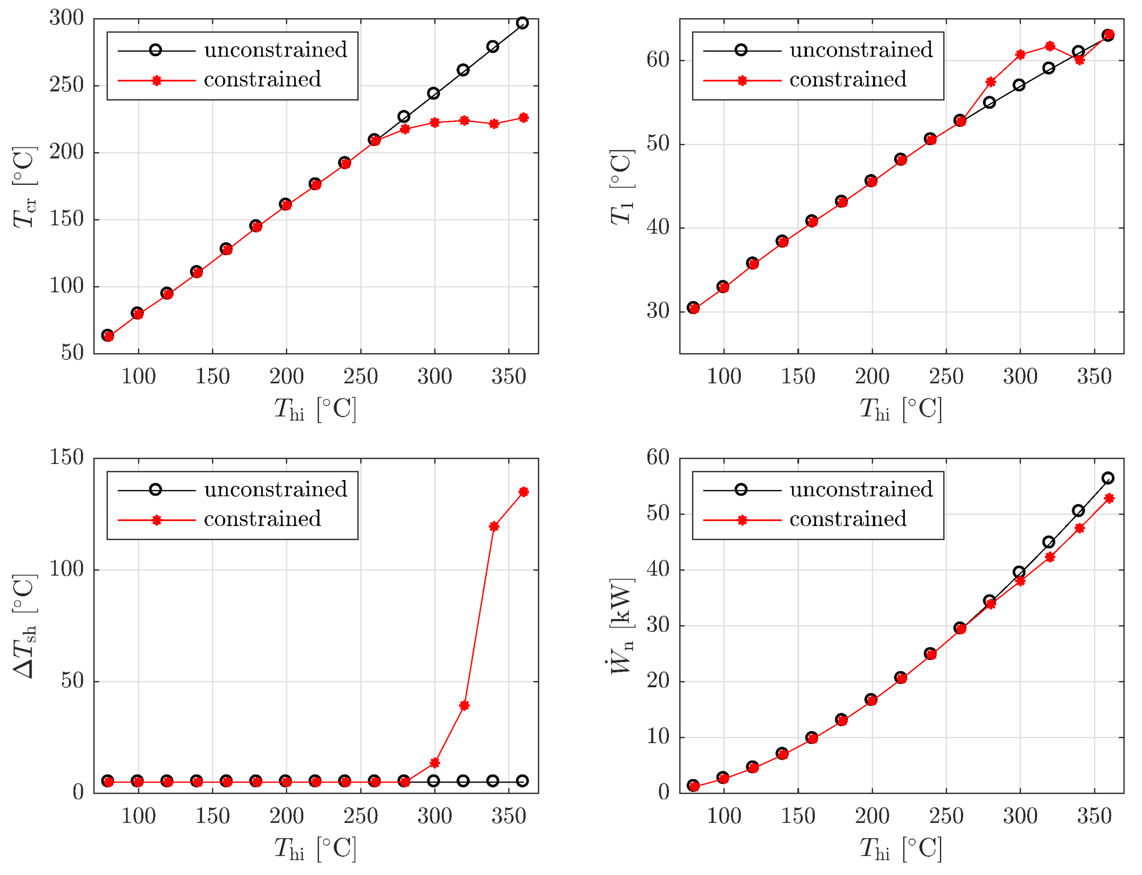
For the first study, the optimisation of the fluid and thermodynamic cycle was conducted for a range of heat-source temperatures according to the bounds given in Table 2. For each heat-source temperature, the optimisation was completed twice; once for an unconstrained condensation pressure ($p_1\ge 5\mathrm{kPa}$), and once for a constrained condensation pressure ($p_1\ge 100\mathrm{kPa}$). It is found that the working fluid is optimised such that $p_{\mathrm{r}}=0.85$ and $\Delta T_{\mathrm{sh}}=5\mathrm{K}$, which reaffirms observations previously made within the literature [20]. The temperature difference $\Delta T_{\mathrm{p}}$ converges to the minimum value that results in a heat-transfer process that does not violate the minimum evaporator pinch point constraint at any point, and the location of this pinch point will be discussed later on. It is also found that the optimal solutions are insensitive to $p_{\mathrm{cr}}$. The remaining optimisation variables are $T_{\mathrm{cr}}$, $\omega$, and $T_1$, and these are plotted in Figure 3, along with the power output from the ORC system.

For the unconstrained cases the optimal values of $T_{\mathrm{cr}}$ and $T_1$ both increase with $T_{\mathrm{hi}}$. In fact, the relationship between $T_{\mathrm{hi}}$ and $T_{\mathrm{cr}}$ is linear, which suggests a strong correlation between these two parameters. In terms of $\omega$, it is observed that, for most cases, $\omega =1$. This reaffirms the point made in Section 2.1, which hypothesised that increasing $\omega$ facilitates a higher pressure ratio across the same temperature difference, and this is advantageous in terms of maximising thermodynamic performance.

The results for the constrained cases show a transition from $\omega =1$ to $\omega =0$ as $T_{\mathrm{hi}}$ increases. At low heat-source temperatures, the optimal constrained cycle is the same as the unconstrained cycle with $\omega =1$. However, as $T_{\mathrm{hi}}$ increases, eventually $\omega =1$ results in a sub-atmospheric condensation pressure. Therefore, it is necessary to reduce $\omega$ to reduce the ORC pressure ratio, and ensure that $p_1\ge 100\mathrm{kPa}$. This continues as $T_{\mathrm{hi}}$ increases further, until $\omega =0$ is reached. After which, the condensation pressure constraint can only be satisfied by increasing $T_1$, as observed in the bottom-left plot in Figure 3. The result of this sudden increase in $T_1$ is a reduction in the optimal $T_{\mathrm{cr}}$, and a reduction in the power output; at $T_{\mathrm{hi}}=360°\mathrm{C}$, the constrained cycle generates 52.3 kW, compared to 56.2 kW by the unconstrained cycle, corresponding to a 6.9% reduction.

For the initial optimisation, $\omega$ was included as an optimisation variable based on the principle that the fluid parameters can be optimised to identify a theoretically optimal fluid, which can then be matched to a real working with similar properties. However, given the tendency of the optimisation to identify fluids with $\omega =1$ or $\omega =0$, it appears that this approach may not result in the identification of feasible fluids. A large proportion of ORC working fluids have acentric factors that are within the range $0.1<\omega <0.5$. From the previous results, it is observed that $T_{\mathrm{cr}}$ and the normal boiling temperature $T_{\mathrm{b}}$ are important parameters governing working-fluid selection. These two parameters have been determined using REFPROP for a number of common ORC working fluids and are plotted in Figure 4. In addition, $T_{\mathrm{b}}$ has been calculated using the Peng–Robinson equation of state for different critical temperatures and acentric factors, assuming $p_{\mathrm{cr}}=30\mathrm{bar}$. It is observed that setting $\omega =0.3$ and $p_{\mathrm{cr}}=30\mathrm{bar}$ is a reasonable approximation that captures the correlation between $T_{\mathrm{cr}}$ and $T_{\mathrm{b}}$ for real working fluids. Therefore, the cycle optimisation study completed can be repeated using these these values. The results from this study are shown in Figure 5, and the saturation curves for the optimal working fluids are shown in Figure 6.

For the unconstrained cases, the optimal cycles again correspond to $p_{\mathrm{r}}=0.85$ and $\Delta T_{\mathrm{sh}}=5\mathrm{K}$. Furthermore, the optimal values of $T_{\mathrm{cr}}$ and $T_1$ share the same trends as observed when $\omega$ was a variable. In comparison, the constrained results are slightly more interesting. Whilst the optimal constrained cycles are identical to the unconstrained cycles for $T_{\mathrm{hi}}\le 260°\mathrm{C}$, at $T_{\mathrm{hi}}>260°\mathrm{C},$ the optimal critical temperatures flatten off and more superheating is applied to the fluid. This is because a further increase in $T_{\mathrm{cr}}$ requires an increased condensation temperature to ensure that the condensation pressure constraint is not violated. This, in turn, causes an increase in the heat-rejection temperature, and a deterioration in the thermodynamic performance of the cycle. Instead, for the high heat-source temperatures, it is better to keep $T_{\mathrm{cr}}$ relatively constant, therefore maintaining a similar condensation temperature, but apply more superheating to the working fluid to best utilise the heat available.

The above discussion can be further complemented by an assessment of the temperature differences within the evaporator at the evaporator inlet (location 2), start of evaporation (location $2^{\prime }$) and evaporator outlet (location 3), and these are shown in Figure 7. It is noted that for the majority of cases all three of these temperature differences are higher than the imposed pinch point, which means that the pinch point is instead located at a point in between location 2 and $2^{\prime }$. None the less, the minimum of the three values shown in Figure 7 is indicative of whether the pinch point is closer to location 2, $2^{\prime }$ or 3. For the unconstrained cycles, it is observed that the pinch point is always located near location $2^{\prime }$. However, for the constrained case the results are more complicated. When $T_{\mathrm{hi}}$ exceeds 260 $°\mathrm{C}$, the pinch point moves towards location 2, which is the result of the flattening off of the optimal critical temperature as the heat-source temperature is increased. Finally, as $T_{\mathrm{hi}}$ approaches 350 $°\mathrm{C}$, the pinch point moves again to location 3, as the degree of superheat becomes sufficiently large.

Using the results, physical working fluids that are good candidates for a particular heat-source temperature can be identified. Considering the unconstrained results for the subcritical cycles (Figure 5), the linear relationship between the $T_{\mathrm{hi}}$ and $T_{\mathrm{cr}}$ can be expressed as:

$$T_{\mathrm{cr}}=0.830T_{\mathrm{hi}}+41.27,$$

(31)

where $T_{\mathrm{cr}}$ and $T_{\mathrm{hi}}$ are both in Kelvin. The coefficients in this expression were obtained using a linear regression, with a resulting coefficient of determination of $R^2=0.9997$. This result is in agreement with other studies reported within the literature that report a link between the heat-source temperature and the critical temperature of the working fluid [10,44,45]. However, within the current paper, the authors have derived a quantitative correlation to identify the optimal critical temperature, based only on the heat-source temperature. Therefore, in the case of an application where the condensation pressure is unconstrained, it is hypothesised that Equation (31) can be used to identify a suitable fluid.

For high temperature applications in which the condensation pressure should be above atmospheric pressure, it is not possible to derive a linear relationship between the critical temperature. This is because working fluids that may be suitable for higher temperature applications generally have sub-atmospheric condensation pressures. Therefore, the introduction of the condensation pressure constraint causes the relationship between $T_{\mathrm{hi}}$ and $T_{\mathrm{cr}}$ to deviate from the linear behaviour. Moreover, as the heat-source temperature increases, the pinch-point location moves, which is a result previously reported in the literature [46,47]. Interestingly, Preißinger and Brüggemann [47] state that for this reason it is not possible to derive a linear relationship between the heat-source temperature and critical temperature. However, it is worth noting that the authors of this previous study focussed specifically on heat-source temperatures in the range of 300 $°\mathrm{C}$ to 600 $°\mathrm{C}$, for which working fluids with high normal boiling temperatures are required. However, in this current study, the focus is on lower temperature applications that range between 80 $°\mathrm{C}$ and 360 $°\mathrm{C}$. It can therefore be stated that Equation (31) is applicable to the range of heat-source temperatures for which condensation can occur above atmospheric pressure, which corresponds to $T_{\mathrm{hi}}<300°\mathrm{C}$.

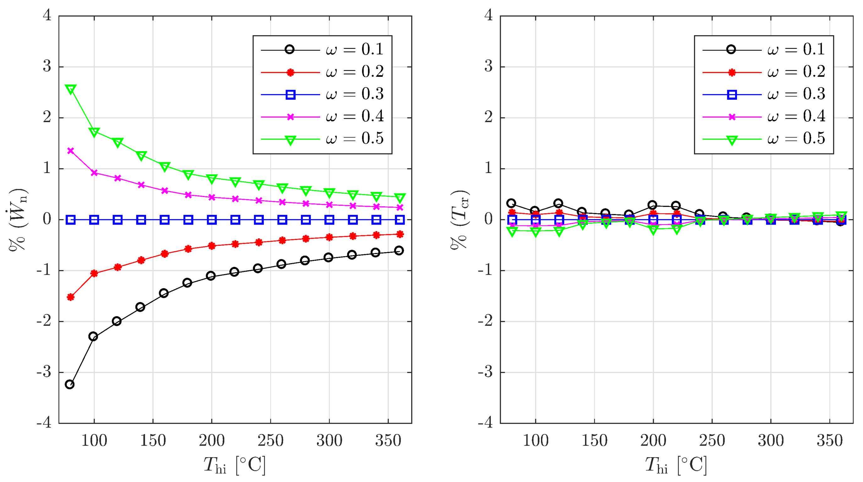
It is worth noting that Equation (31) has been obtained assuming $\omega =0.3$. To investigate the sensitivity of the results to variations in $\omega$, a sensitivity analysis considering the effect of $\omega$ on the net power output and fluid critical temperature has been conducted. The results are shown in Figure 8. From this, it is observed that $\omega$ has very little effect on the optimal working-fluid critical temperature. Moreover, for heat-source temperatures greater than 100 $°\mathrm{C}$, the percentage difference in the power output compared to a working fluid with $\omega =0.3$ is less than 2%. Therefore, the optimisation is not that sensitive to variations in $\omega$.

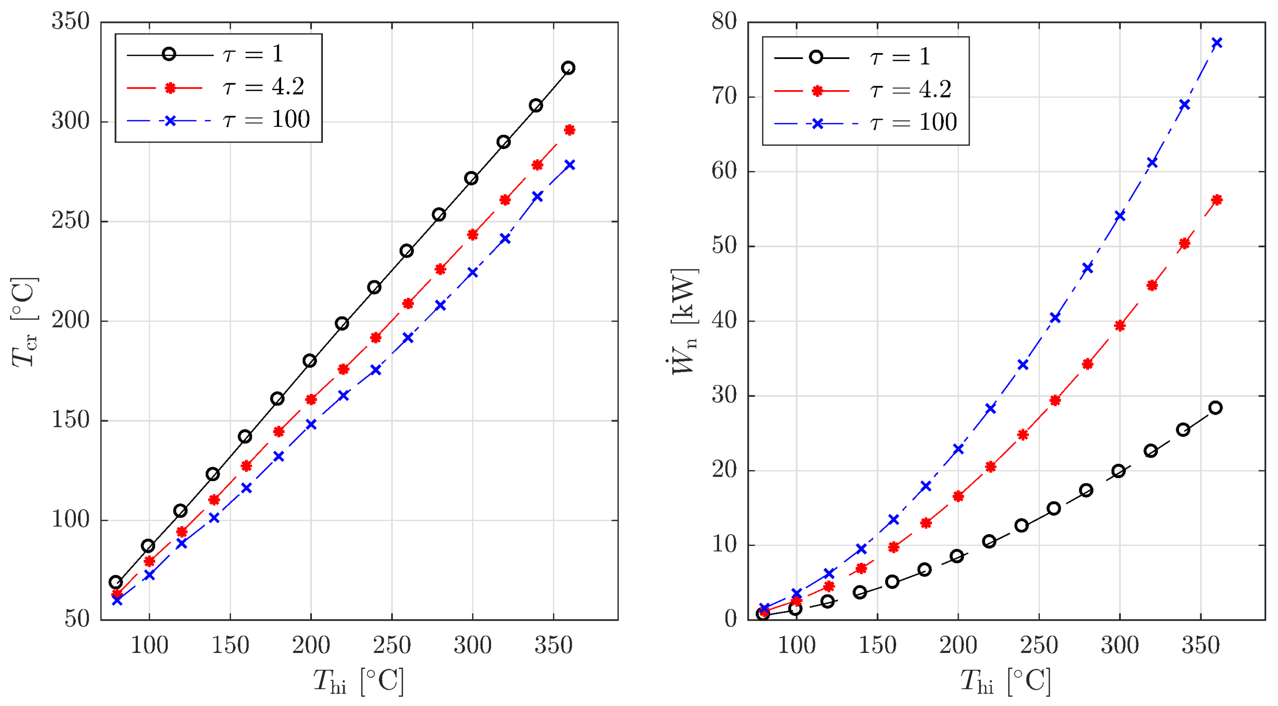
It is also worth noting that Equation (31) is based on a fixed heat-capacity ratio of $\tau ={\left(\dot{m}{c}_p\right)}_{\mathrm{c}}/{\left(\dot{m}{c}_p\right)}_{\mathrm{h}}=4.2$. Therefore, the same optimisation study for the subcritical cycle has been repeated for $\tau =1$ and $\tau =100$, and the results are shown in Figure 9. It is observed that reducing $\tau$ results in an optimal working fluid with a higher critical temperature, whilst increasing $\tau$ results in an optimal working fluid with a lower critical temperature. The maximum deviation between the optimal critical temperature for $\tau =100$ and $\tau =4.2$ is only 3.8%. For $\tau =1$, the maximum deviation is slightly larger (5.4%); however, this is a relatively extreme case as a low heat-capacity ratio results in a significantly reduced power output, as shown in the right-hand plot of Figure 9.

Ultimately, the results in Figure 9 suggest that the optimal critical temperature of a working fluid for a subcritical, non-recuperated ORC is not significantly affected by the relative size of the available heat sink, compared to the heat source. Moreover, it is reiterated that from a thermodynamic perspective the optimal working fluid and cycle operating conditions are independent of the heat-source heat-capacity rate; in other words, the only parameter that changes as the size of the heat-source changes is the working-fluid mass-flow rate. It can therefore be concluded that Equation (31) is broadly applicable to waste-heat recovery applications where the heat-source temperature is below 300 $°\mathrm{C}$, and can be used to identify a suitable working fluid for a subcritical, non-recuperated ORC, based on only the heat-source temperature.

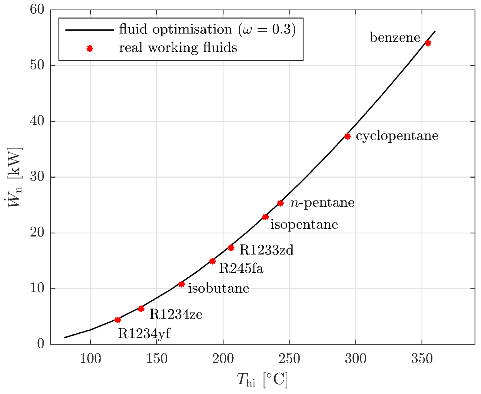
To confirm the validity of Equation (31), nine physical fluids have been considered with critical temperatures ranging between $95°\mathrm{C}$ (R1234yf) and $289°\mathrm{C}$ (benzene). Working backwards, the optimal heat-source temperatures for these fluids have been identified using Equation (31). For each working fluid, a cycle optimisation was then completed using the Peng–Robinson equation of state model, with the values for $T_{\mathrm{cr}}$, $p_{\mathrm{cr}}$, $\omega$, A, B and C being obtained using REFPROP. The results from these simulations are compared to the theoretically optimal cycles in Figure 10. The results show a maximum deviation of 18% between the theoretical and real working fluids when $T_{\mathrm{hi}}<120°\mathrm{C}$. At higher temperatures, the deviation is less significant, reducing to below 5% for $T_{\mathrm{hi}}>220°\mathrm{C}$. It is observed that for the nine working fluids the same optimal cycles are identified with $p_{\mathrm{r}}=0.85$ and $\Delta T_{\mathrm{sh}}=5\mathrm{K}$. It is also noted that the only fluid with a sub-atmospheric pressure is benzene, which has an optimal condensation pressure of 57 kPa. Therefore, since cyclopentane appears suitable for heat-source temperatures of 300 $°\mathrm{C}$, and has a condensation pressure greater than atmospheric pressure, these results confirm that Equation (31) can be used to identify the critical temperature of an optimal working fluid for a subcritical cycle, allowing maximum power to be generated from a defined heat source, provided that $T_{\mathrm{hi}}<300°\mathrm{C}$. Therefore, this correlation can be used to narrow the search space during working-fluid selection for heat-source tempeatures within range. Future research should investigate the validity of this correlation for higher temperature heat sources.

The Peng–Robinson model can be validated by completing the same optimisation for the nine defined working fluids using REFPROP directly. It is again observed that the optimal cycles correspond to $p_{\mathrm{r}}=0.85$ and $\Delta T_{\mathrm{sh}}=5\mathrm{K}$. Furthermore, the maximum deviations between the optimal condensation temperatures and expander inlet temperatures obtained using Peng–Robinson and REFPROP are 0.41% and 0.1% respectively. After converting these temperatures into the corresponding condensation pressures, it is observed that the Peng–Robinson model over predicts the condensation pressure, with a maximum deviation of 3.5% being observed for R1234ze. As a consequence, the Peng–Robinson model results in power outputs that are slightly higher than those obtained using REFPROP, with a maximum deviation of 5.9%. These deviations are in line with similar comparisons reported within the literature [24,25]. However, despite this deviation, it is apparent that both the Peng–Robinson and REFPROP models identify the same optimal values for the optimisation variables for each working fluid. This confirms that the Peng–Robinson model is suitable for identifying the optimal cycle for a given working fluid and heat-source temperature.

Using the optimisation setup based on REFPROP, it is possible to investigate the result of selecting a physical working fluid with a different critical temperature to the theoretically optimal value identified using the Peng–Robinson model. For this, the optimal heat-source temperatures for R1234yf, isopentane, R1233zd and n-pentane have been considered and the optimisation repeated with different working fluids. The results are shown in Figure 11. It can be observed that selecting a working fluid with either a lower critical temperature, or higher critical temperature results in a reduction in the maximum power that can be output from the system. More specifically, the fluids that produce the second largest power output correspond to a reduction in power output of 7.2%, 10.0%, 7.9% and 6.7% compared to optimal working fluid. In other words, this confirms that using Equation (31), based on the results from the Peng–Robinson model, correctly identifies the optimal physical working fluids that results in the maximum power output from a given heat-source temperature.

5.2. Turbine Results

In the previous section, a generalised approach to working-fluid selection has been implemented using the Peng–Robinson equation of state. This has identified optimal working fluids and cycle operating conditions for heat-source temperatures ranging between $122°\mathrm{C}$ and $343°\mathrm{C}$. The next step is to establish how this variation in heat-source temperature affects both the design and performance of the radial turbine.

As discussed in Section 3, the turbine model requires properties such as molar mass and viscosity, which cannot be determined using the Peng–Robinson equation of state. Instead, the turbine optimisation has been conducted with the nine working fluids previously considered, and REFPROP was utilised for the fluid thermo-physical properties. Therefore, the turbine analysis is not as general as the approach adopted when evaluating the thermodynamic cycle. Nonetheless, the use of Equation (31) to transition from a theoretical fluid to a physical fluid ensures that the fluids being considered are an accurate representation of the theoretical fluid for a particular heat source. Therefore, a generalised assessment of the turbine performance across a range of heat-source temperatures is still possible.

For each working fluid and optimal cycle identified in the previous section, the turbine optimisation process described in Section 4.3 was applied. The cycle conditions were set to the optimal cycle subcritical cycle conditions that were identified when the cycle optimisation was completed using REFPROP. Furthermore, in order to conduct a fair comparison between the different working fluids, the mass-flow rate was scaled such that the net power output from the ORC is approximately 25 kW for each working fluid. The design specification for each turbine is summarised in

Table 6. Thermodynamic specification for the nine turbine designs for the optimal subcritical cycle.

Working Fluid	${\mathit{T}}_{\mathbf{hi}}$ $\mathbf{°}\mathbf{C}$	${\mathit{T}}_{\mathbf{03}}$ $\mathbf{°}\mathbf{C}$	${\mathit{p}}_{\mathbf{03}}$ bar	${\mathit{p}}_{\mathbf{6}}$ bar	${\dot{\mathit{m}}}_{\mathbf{w}}$ kg/s
R1234yf	120.6	91.7	28.75	8.99	1.910
R1234ze	138.2	106.2	30.90	7.14	1.393
isobutane	168.7	130.1	30.85	5.47	0.527
R245fa	192.0	150.2	31.03	2.88	0.786
R1233zd	206.0	161.2	30.37	2.63	0.742
isopentane	232.0	181.8	28.71	1.93	0.325
n-pentane	243.3	191.1	28.65	1.56	0.293
cyclopentane	293.9	231.9	38.86	1.28	0.231
benzene	354.6	281.0	41.71	0.58	0.181

.

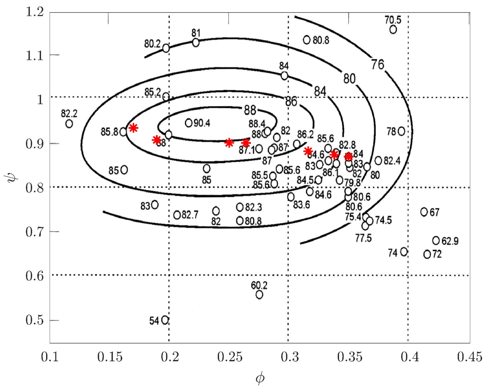
Before discussing the results, it is noted that the optimisation did not converge for the cyclopentane and benzene cases. The reason for this will be discussed at the end of this section. For the working fluids that did converge, it was found that the hub/shroud diameter ratio was on the lower limit (i.e., $d_{5\mathrm{h}}/d_{5\mathrm{s}}=0.35$), suggesting it is advantageous to reduce the hub diameter as much as possible. However, crowding at the rotor hub should be avoided, and this should be verified during a more detailed design phase. In terms of the inlet/outlet diameter ratio, the optimal values range between 0.56 and 0.64, and these agree well with results reported in Ref. [43]. The remaining two optimisation variables are the blade loading and flow coefficients. These two parameters have been well correlated against turbine isentropic efficiency, providing a good basis for comparison. In Figure 12, the optimal values of $\psi$ and $\varphi$ for each working fluid have been superimposed onto the chart found in Ref. [39]. It is observed that the optimal turbine designs correlate very well with performance data within the literature. More specifically, as the heat-source temperature increases, the optimal value of $\psi$ increases, whilst the optimal value of $\varphi$ reduces. Therefore, the optimal design point moves from the bottom-right corner to the top-left corner of the design chart as the heat-source temperature increases. The total-to-static isentropic efficiency also reduces slightly as heat-source temperatures increases, with a maximum of ${\eta }_{\mathrm{ts}}=85.2\%$ for the R1234yf turbine, and a minimum of ${\eta }_{\mathrm{ts}}=82.5\%$ for the n-pentane turbine. The corresponding isentropic velocity ratio for the optimal turbines also reduce as the heat-source temperature increases, reducing from $\nu =0.698$ for R1234yf, to $\nu =0.673$ for n-pentane.

The rotor geometry for three of the optimal turbine designs are plotted in Figure 13, with heat-source temperature increasing from left-to-right. There is a significant reduction in rotor inlet blade height from 3.47 mm for the R1234yf turbine, to 1.56 mm for the n-pentane turbine as the heat-source temperature increases. This is because a higher heat-source temperature corresponds to higher pressure ratio, and therefore density ratio across the turbine. Therefore, the flow area at the rotor inlet, relative to the rotor outlet flow area, must reduce.

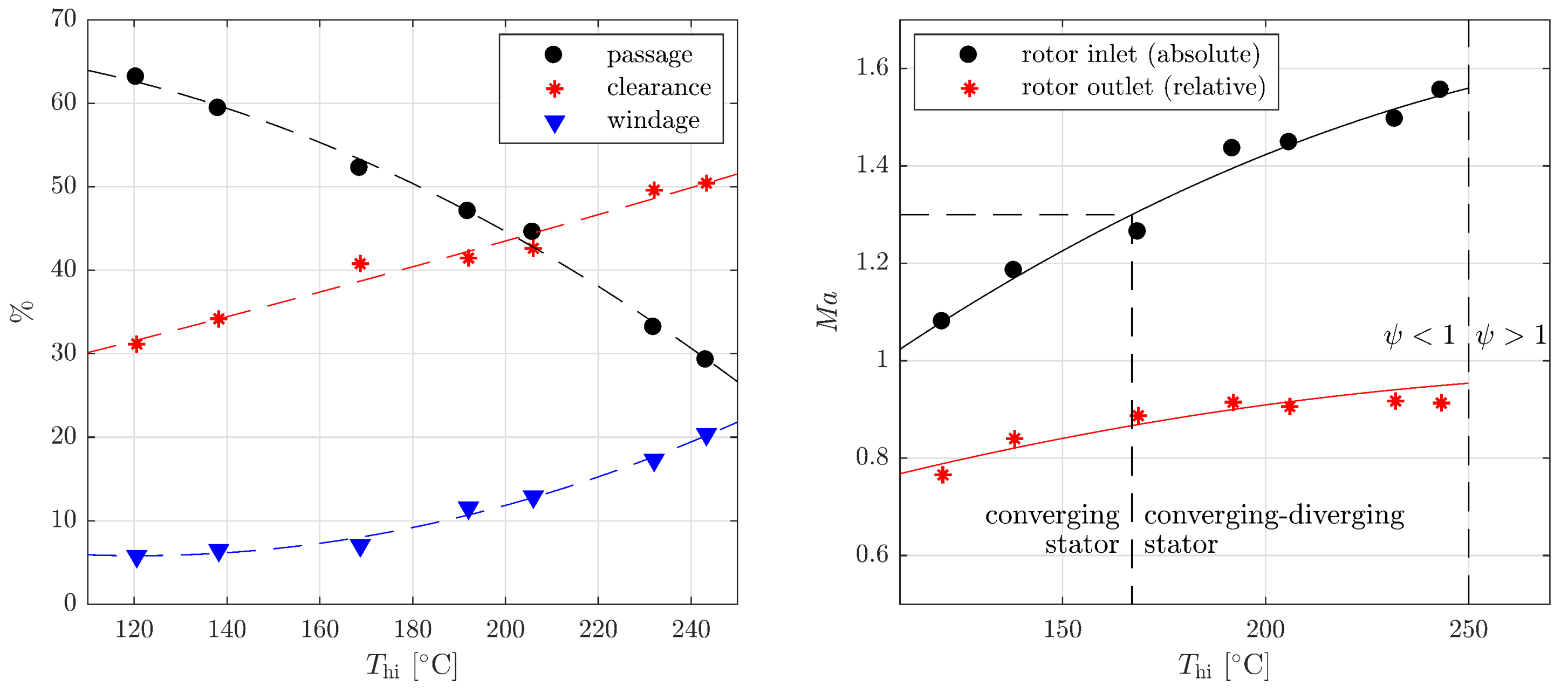
On the left-hand side of Figure 14, the breakdown of the main losses within the rotor are plotted as a function of the heat-source temperature. The trailing-edge loss is not included since this is a separate loss that applies downstream of the rotor. However, it is observed that the trailing-edge loss increases with increasing $T_{\mathrm{hi}}$, but this loss is small, relative to the other three loss mechanisms. The results shown in Figure 14 are useful to understand the role that the different loss mechanisms have in optimal turbine performance. For a low-temperature ORC system, designed for $T_{\mathrm{hi}}=120°\mathrm{C}$ and operating with R1234yf, the dominant loss mechanism is the passage loss, accounting for 63% of the loss, whilst the clearance and windage losses account for 31% and 6%, respectively. For a high-temperature ORC system, designed for $T_{\mathrm{hi}}=240°\mathrm{C}$ and operating with n-pentane, the clearance loss becomes more dominant owing to the reduced rotor inlet blade height. In this instance, the clearance loss accounts for 51% of the loss, whilst the contribution from the passage loss reduces to 29%, and the windage loss contribution increases to 20%. Ultimately, it is believed that Figure 14 could be instrumental in identifying target areas for future research. For example, targeting reductions in the passage loss for low-temperature ORC turbines, and reducing the clearance loss associated with higher-temperature turbines, could be the most direct route to efficiency improvements for small-scale ORC turbines.

The maximum absolute and relative Mach numbers within the turbine, which occur at the rotor inlet and rotor outlet respectively, have also been plotted in Figure 14. The rotor inlet absolute Mach number has an important impact on the stator design. Below $Ma<1.3$, a stator with a converging profile can be used to accelerate the flow to the required speed, albeit with $Ma>1$ being obtained within the rotor-stator interspace. However, for $Ma>1.3,$ a converging-diverging is required, which has a more complex design, and cannot easily accommodate off-design operating conditions. The transition from a converging to a converging-diverging stator occurs when the heat-source temperature exceeds $165°\mathrm{C}$. In terms of the rotor outlet relative Mach number, all of the optimal turbine designs are below $Ma<1$. This is not surprising since this was a constraint during the optimisation. However, as the heat-source temperature increases, the rotor outlet relative Mach number also increases, and therefore this must be carefully considered for higher-temperature ORC systems.

Referring to Refs. [31,32], it was shown that high expansion ratios and operating close to the critical point results in a reduction in turbine efficiency. Within the current paper, it has been shown that the turbine efficiency for the optimal cycles reduces from 85.2% to 82.5% as the heat-source temperature increases, which is consistent with the findings in these previous studies. On the other hand, all of the optimal cycles considered within this paper have high reduced pressures ($p_{\mathrm{r}}=0.85$). Therefore, it may be possible to improve turbine efficiency by reducing the evaporation pressure, or selecting a fluid with a higher critical temperature. However, as shown in Figure 11, doing so can be expected to lead to a reduction in the maximum power output from the cycle. Therefore, it is necessary to identify whether the reduction in turbine efficiency that is introduced by operating close the critical point is offset by the increase in the net power output; this interplay should be investigated further.

Finally, it is worth considering the cyclopentane and benzene cases, for which the turbine optimisation did not converge. In these cases, it was not possible to identify a turbine design that met all of the defined constraints. Considering Figure 12, and the accompanying discussion, it was found that the optimal value of $\psi$ increases as $T_{\mathrm{hi}}$ increases, with $\psi =0.940$ for n-pentane. This suggests that, for higher heat-source temperatures, it would be necessary to further increase $\psi$ to be above 1, which, in turn, would require a forward-swept blade instead of the radially-fibered blade that is considered within this study. Therefore, it appears that the operating boundary for a conventional, radial-fibered blade with $\psi <1$ occurs at $T_{\mathrm{hi}}=250°\mathrm{C}$, as indicated in Figure 14.

6. Conclusions

Many existing ORC studies arrive at an optimal working fluid and turbine design considering only the specific application in question. However, a generalised approach is more meaningful and could facilitate a standardised, and streamlined, design process. In this paper, it has been found that, by coupling the Peng–Robinson equation of state with an ORC model, and then optimising the working-fluid parameters alongside the thermodynamic cycle, the characteristics of an optimal working fluid can be identified. Furthermore, this information can be used to identify potential working-fluid candidates. More specifically, a linear correlation has been derived between the heat-source temperature and the optimal critical temperature, which is applicable for heat-source temperatures below 300 $°\mathrm{C}$.

Regarding turbine design, it is found that, as the heat-source temperature increases, the optimal blade-loading coefficient increases, whilst the flow coefficient reduces. Moreover, at heat-source temperatures exceeding 250 $°\mathrm{C},$ a forward-swept blade is required to accommodate blade-loading coefficients exceeding 1. It is also observed that, as the heat-source temperature exceeds 165 $°\mathrm{C},$ a converging-diverging stator is necessary to achieve the necessary supersonic conditions at the rotor inlet. In terms of rotor performance, it is found that, for a 120 $°\mathrm{C}$ heat source, the passage loss accounts for over 60% of the total loss within the rotor. Comparatively, for a 250 $°\mathrm{C}$ heat source, the clearance loss is dominant, accounting for over 50% of the total loss. These two results can be used inform the most direct routes to efficiency improvements in small-scale ORC turbines for different heat-source temperatures. Moreover, these results may be broadly applicable to larger-scale systems, although the relative clearance loss would be expected to reduce, owing to smaller relative clearance gaps.

In order to improve the performance of ORC systems, it is necessary to further characterise ORC turbine performance using more advanced numerical and experimental techniques. Currently, as part of the NextORC project [48], a closed-loop supersonic wind tunnel for organic fluids is currently being designed and commissioned. Therefore, the optimal working fluids and turbine designs identified within this paper will form the base cases that will be studied as part of this future work.

References

- World Overview of the Organic Rankine Cycle Technology. Available online: http://orc-world-map.org/ (accessed on 31 August 2017).
- Environmental Investigation Agency (EIA). Kigali Amendment to the Montreal Protocol: A Crucial Step in the Fight Against Catastrophic Climate Change. Available online: https://eia-international.org/wp-content/uploads/EIA-Kigali-Amendment-to-the-Montreal-Protocol-FINAL.pdf (accessed on 31 August 2017).
- Lemmon, E.; Huber, M.; McLinden, M. NIST Standard Reference Database 23: Reference Fluid Thermodynamic and Transport Properties-REFPROP, Version 9.1; National Institute of Standards and Technology: Gaithersburg, MD, USA, 2013.
- Bell, I.H.; Wronski, J.; Quoilin, S.; Lemort, V. Pure and pseudo-pure fluid thermophysical property evaluation and the open-source thermophysical property library CoolProp. Ind. Eng. Chem. Res. 2014, 53, 2498–2508. [Google Scholar] [CrossRef] [PubMed] [Green Version]
- Saleh, B.; Koglbauer, G.; Wendland, M.; Fischer, J. Working fluids for low-temperature organic Rankine cycles. Energy 2007, 32, 1210–1221. [Google Scholar] [CrossRef]
- Tchanche, B.F.; Papadakis, G.; Lambrinos, G.; Frangoudakis, A. Fluid selection for a low-temperature solar organic Rankine cycle. Appl. Therm. Eng. 2009, 29, 2468–2476. [Google Scholar] [CrossRef]
- Drescher, U.; Brüggemann, D. Fluid selection for the organic Rankine cycle (ORC) in biomass power and heat plants. Appl. Therm. Eng. 2007, 27, 223–228. [Google Scholar] [CrossRef]
- Schwoebel, J.A.H.; Preißinger, M.; Brüggemann, D.; Klamt, A. High-throughput screening of working fluids for the organic Rankine cycle (ORC) based on conductor-like screening model for realistic solvation (COSMO-RS) and thermodynamic process simulations. Ind. Eng. Chem. Res. 2017, 56, 788–798. [Google Scholar] [CrossRef]
- Preißinger, M.; Schwoebel, J.A.H.; Klamt, A.; Brüggemann, D. Multi-criteria evaluation of several million working fluids for waste heat recovery by means of organic Rankine cycle in passenger cars and heavy-duty trucks. Appl. Energy 2017, 206, 887–899. [Google Scholar] [CrossRef]
- Vivian, J.; Manente, G.; Lazzaretto, A. A general framework to select working fluid and configuration of ORCs for low-to-medium temperature heat sources. Appl. Energy 2015, 156, 727–746. [Google Scholar] [CrossRef]
- Joback, K.G.; Reid, R.C. Estimation of pure-component properties from group-contributions. Chem. Eng. Commun. 1987, 57, 233–243. [Google Scholar] [CrossRef]
- Chapman, W.G.; Gubbins, K.E.; Jackson, G.; Radosd, M. New reference equation of state for associating liquids. Ind. Eng. Chem. Res. 1990, 29, 1709–1721. [Google Scholar] [CrossRef]
- Papadopoulos, A.I.; Stijepovic, M.; Linke, P. On the systematic design and selection of optimal working fluids for organic Rankine cycles. Appl. Therm. Eng. 2010, 30, 760–769. [Google Scholar] [CrossRef]
- Palma-Flores, O.; Flores-Tlacuahuac, A.; Canseco-Melchor, G. Simultaneous molecular and process design for waste heat recovery. Energy 2016, 99, 32–47. [Google Scholar] [CrossRef]
- Cignitti, S.; Andreasen, J.G.; Haglind, F.; Woodley, J.M.; Abildskov, J. Integrated working fluid-thermodynamic cycle design of organic Rankine cycle power systems for waste heat recovery. Appl. Energy 2017, 203, 442–453. [Google Scholar] [CrossRef]
- Lampe, M.; Stavrou, M.; Bu, H.M.; Gross, J.; Bardow, A. Simultaneous optimization of working fluid and process for organic Rankine cycles using PC-SAFT. Ind. Eng. Chem. Res. 2014, 53, 8821–8830. [Google Scholar] [CrossRef]
- Lampe, M.; Stavrou, M.; Schilling, J.; Sauer, E.; Gross, J.; Bardow, A. Computer-aided molecular design in the continuous-molecular targeting framework using group-contribution PC-SAFT. Comput. Chem. Eng. 2015, 81, 278–287. [Google Scholar] [CrossRef]
- Gross, J.; Sadowski, G. Modeling polymer systems ising the perturbed-chain statistical associating fluid theory equation of state. Ind. Eng. Chem. Res. 2002, 41, 1084–1093. [Google Scholar] [CrossRef]
- Schilling, J.; Lampe, M.; Bardow, A. 1-Stage CoMT-CAMD: An approach for integrated design of ORC process and working fluid using PC-SAFT. Chem. Eng. Sci. 2016, 159, 217–230. [Google Scholar] [CrossRef]
- White, M.; Oyewunmi, O.; Haslam, A.; Markides, C. Industrial waste-heat recovery through integrated computer-aided working-fluid and ORC system optimisation using SAFT-γ Mie. Energy Convers. Manag. 2017, 150, 851–869. [Google Scholar] [CrossRef]
- Luján, J.M.; Serrano, J.R.; Dolz, V.; Sánchez, J. Model of the expansion process for R245fa in an organic Rankine cycle (ORC). Appl. Therm. Eng. 2012, 40, 248–257. [Google Scholar] [CrossRef]
- Peng, D.Y.; Robinson, D.B. A new two-constant equation of state. Ind. Eng. Chem. Fundam. 1976, 15, 59–64. [Google Scholar] [CrossRef]
- Soave, G. Equilibrium constants from a modified Redlich-Kwong equation of state. Chem. Eng. Sci. 1972, 27, 1107–1203. [Google Scholar] [CrossRef]
- Brignoli, R.; Brown, J.S. Organic Rankine cycle model for well-described and not-so-well-described working fluids. Energy 2015, 86, 93–104. [Google Scholar] [CrossRef]
- Su, W.; Zhao, L.; Deng, S. Developing a performance evaluation model of organic Rankine cycle for working fluids based on the group contribution method. Energy Convers. Manag. 2017, 132, 307–315. [Google Scholar] [CrossRef]
- Frutiger, J.; Bell, I.; O’Connell, J.; Kroenlein, K.; Abildskov, J.; Sin, G. Uncertainty assessment of equations of state with application to an organic Rankine cycle. Mol. Phys. 2017, 115, 1225–1244. [Google Scholar] [CrossRef]
- Oudkerk, J.F.; Dickes, R.; Dumont, O.; Lemort, V. Experimental performance of a piston expander in a small-scale organic Rankine cycle. In IOP Conference Series: Materials Science and Engineering; IOP Publishing: Bristol, UK, 2015; Volume 90. [Google Scholar]
- Casati, E.; Vitale, S.; Pini, M.; Persico, G.; Colonna, P. Centrifugal turbines for mini-ORC power systems. J. Eng. Gas Turbines Power 2014, 136, 122607. [Google Scholar] [CrossRef]
- Fiaschi, D.; Manfrida, G.; Maraschiello, F. Design and performance prediction of radial ORC turboexpanders. Appl. Energy 2015, 138, 517–532. [Google Scholar] [CrossRef]
- Costall, A.; Gonzalez Hernandez, A.; Newton, P.; Martinez-Botas, R. Design methodology for radial turbo expanders in mobile organic Rankine cycle applications. Appl. Energy 2015, 157, 729–743. [Google Scholar] [CrossRef]
- Lio, L.D.; Manente, G.; Lazzaretto, A. Predicting the optimum design of single stage axial expanders in ORC systems: Is there a single efficiency map for different working fluids? Appl. Energy 2016, 167, 44–58. [Google Scholar] [CrossRef]
- Lio, L.D.; Manente, G.; Lazzaretto, A. A mean-line model to predict the design efficiency of radial inflow turbines in organic Rankine cycle (ORC) systems. Appl. Energy 2017, 205, 187–209. [Google Scholar] [CrossRef]
- Meroni, A.; Andreasen, J.G.; Pierobon, L.; Haglind, F. Optimization of cycle and expander design of an organic Rankine cycle using multi-component working fluids. In Proceedings of the ASME Turbo Expo 2016: Turbomachinery Technical Conference and Exposition, Seoul, Korea, 13–17 June 2016. [Google Scholar]
- Al Jubori, A.M.; Al-Dadah, R.K.; Mahmoud, S.; Daabo, A. Modelling and parametric analysis of small-scale axial and radial-outflow turbines for organic Rankine cycle applications. Appl. Energy 2017, 190, 981–996. [Google Scholar] [CrossRef]
- Landelle, A.; Tauveron, N.; Haberschill, P.; Revellin, R.; Colasson, S. Organic Rankine cycle design and performance comparison based on experimental database. Appl. Energy 2017, 204, 1172–1187. [Google Scholar] [CrossRef]
- Poling, B.E.; Prausnitz, J.M.; O’Connell, J.P. The Properties of Gases and Liquids, 5th ed.; McGraw-Hill: New York, NY, USA, 2001; p. 768. [Google Scholar]
- Stryjek, R.; Vera, J. PRSV: An improved Peng–Robinson equation of state for pure compounds and mixtures. Can. J. Chem. Eng. 1986, 64, 323–333. [Google Scholar] [CrossRef]
- Chen, H.; Goswami, D.Y.; Stefanakos, E.K. A review of thermodynamic cycles and working fluids for the conversion of low-grade heat. Renew. Sustain. Energy Rev. 2010, 14, 3059–3067. [Google Scholar] [CrossRef]
- Baines, N.C. Part 3: Radial Turbine Design. In Axial and Radial Turbines; Chapter 7–9; Concepts NREC: White River Junction, VT, USA, 2003. [Google Scholar]
- Aungier, R.H. Turbine Aerodynamics: Axial-flow and Radial-inflow Turbine Design and Analysis, 1st ed.; ASME Press: New York, NY, USA, 2006. [Google Scholar]
- Roelke, R.J. Miscellaneous Losses. In Turbine Design and Application; Chapter 8; NASA: Washington, DC, USA, 1972; p. 390. [Google Scholar]
- The Mathworks, Inc. Global Optimisation Toolbox. Available online: https://uk.mathworks.com/help/gads/index.html?searchHighlight=global (accessed on 31 August 2017).
- Dixon, S.L. Fluid Mechanics and Thermodynamics of Turbomachinery, 5th ed.; Butterworth-Heinemann: Woburn, MA, USA, 2005. [Google Scholar]
- Lie, W.; Meinel, D.; Gleinser, M.; Wieland, C.; Spliethoff, H. Optimal heat source temperature for thermodynamic optimisation of sub-critical organic Rankine cycles. Energy 2015, 88, 897–906. [Google Scholar] [CrossRef]
- Zhai, H.; An, Q.; Shi, L. Analysis of the quantitative correlation between the heat source temperature and the critical temperature of the optimal pure working fluid for subcritical organic Rankine cycles. Appl. Therm. Eng. 2016, 99, 383–391. [Google Scholar] [CrossRef]
- Braimakis, K.; Preißinger, M.; Brüggemann, D.; Karellas, S. Low grade waste heat recovery with subcritical and supercritical organic Rankine cycle based on natural refrigerants and their binary mixtures. Energy 2015, 88, 80–92. [Google Scholar] [CrossRef]
- Preißinger, M.; Brüggemann, D. Thermoeconomic evaluation of modular organic Rankine cycles for waste heat recovery over a broad range of heat source temperatures and capacities. Energies 2017, 10, 269. [Google Scholar] [CrossRef]
- NextORC: Fundamental Studies on Organic Rankine Cycle Expanders. Available online: www.city.ac.uk/NextORC (accessed on 15 November 2017).
Figure 1.
Effect of , A, B and C on the thermodynamic behaviour of a working fluid with and . For the top two plots, , whilst for the bottom plot .
Figure 2.
Notation used to describe the thermodynamic cycle (left) and a radial turbine (right). In the left figure the red and blue lines correspond to the heat source and heat sink temperature profiles respectively, and the magenta lines represent the thermodynamic cycle.
Figure 3.
Optimal fluid and cycle parameters for different heat-source temperatures for an unconstrained () and constrained () condensation pressure with included as an optimisation variable.
Figure 4.
Critical temperature and boiling temperature of common working fluids available within the REFPROP program (circles) and the same parameters obtained using the Peng–Robinson equation of state for different values of with (lines).
Figure 5.
Optimal working fluid and cycle parameters for different heat-source temperatures for a subcritical cycle. Results obtained for an unconstrained () and constrained () condensation pressure with .
Figure 6.
Saturation curves for the optimal working fluids obtained from the cycle optimisation for the unconstrained (left) and constrained (right) condensation pressure cases with .
Figure 7.
Temperature differences within the evaporator for the optimal cycles obtained for the unconstrained (left) and constrained (right) condensation pressure cases with .
Figure 8.
Sensitivity analysis on the effect of on (left) and (right) for an unconstrained () subcritical ORC system for different heat-source temperatures. Results are compared to optimal systems for .
Figure 9.
Optimal critical temperature (left) and power output (right) as a function of heat-source temperature for different heat-capacity ratios (). Results obtained for an unconstrained ( kPa) subcritical cycle.
Figure 10.
Comparison between the results from an integrated working-fluid and cycle optimisation with (line) and cycle optimisations completed for predefined working fluids (markers) for subcritical cycles. For all optimisation studies, the condensation pressure is unconstrained.
Figure 11.
Effect of selecting a working fluid with a non-optimal critical temperature on the power output from the system. In each plot, fluids are plotted in order of increasing critical temperature, with the dark blue bars representing the optimal fluid identified using the Peng–Robinson model, from left to right: , 169 , 206 and 243 .
Figure 12.
Comparison between the optimal turbine designs (red markers) and other turbine designs (white circles) reported within the literature in terms of the blade-loading coefficient and the flow coefficient ; original plot taken from Ref. [39].
Figure 13.
Meridional profiles for three of the optimal turbine designs.
Figure 14.
Breakdown of the passage, clearance and windage loss within the rotor (left) and variation in the rotor inlet absolute Mach number and rotor outlet relative Mach number (right) for the nine optimal turbine designs, plotted as a function of heat-source temperature.