Verification and Validation of a Low-Mach-Number Large-Eddy Simulation Code against Manufactured Solutions and Experimental Results


1
State Key Laboratory of Clean Energy Utilization, Zhejiang University, Hangzhou 310027, China
2
School of Engineering and Technology, University of Hertfordshire, Herts AL10 9AB, UK
*
Authors to whom correspondence should be addressed.
Energies 2018, 11(4), 921; https://doi.org/10.3390/en11040921
Submission received: 28 March 2018
/
Revised: 7 April 2018
/
Accepted: 7 April 2018
/
Published: 13 April 2018
(This article belongs to the Special Issue Fuels of the Future)
Abstract
:To investigate turbulent reacting flows, a low-Mach number large-eddy simulation (LES) code called ‘LESsCoal’ has been developed in our group. This code employs the Germano dynamic sub-grid scale (SGS) model and the steady flamelet/progress variable approach (SFPVA) on a stagger-structured grid, in both time and space. The method of manufactured solutions (MMS) is used to investigate the convergence and the order of accuracy of the code when no model is used. Finally, a Sandia non-reacting propane jet and Sandia Flame D are simulated to inspect the performance of the code under experimental setups. The results show that MMS is a promising tool for code verification and that the low-Mach-number LES code can accurately predict the non-reacting and reacting turbulent flows. The validated LES code can be used in numerical investigations on the turbulent combustion characteristics of new fuel gases in the future.
1. Introduction
With the rapid development of computer hardware and parallel computing technology, high-fidelity simulation techniques, especially the large-eddy simulation, have become increasingly efficient and competitive. They now play an important role in the research field of complex turbulent reacting flows [1,2], and have been widely used in the design, analysis, and optimization of engineering systems [3,4,5]. For computational studies, it is important to make sure that the simulation results are accurate and that the computational code can be used for prediction. Therefore, the validation of a computational code is a crucial step in computational research [6]. The validated code can then be used in numerical investigations on the turbulent combustion characteristics of new fuel gases, for example, the syngas produced from the gasification of coal and biomass.
Verification is defined as the substantiation that the numerical methods implemented in a code can represent the original conceptual algorithm correctly; while validation is the assurance that the code can provide an accurate prediction compared with widely acknowledged and convincing experimental data. On the verification side, the method of manufactured solutions (MMS) appears as a comparatively accessible method for code verification to ensure that all of the numerical methods are correct and that the governing equations are correctly solved. Using MMS, the numerical results of a computational fluid dynamics (CFD) code can be compared to the exact analytical solutions under a specific designed condition. Hence, the performance of the numerical methods in the code can be judged and the order of accuracy of the code can be determined. MMS has been widely used for verifying both incompressible and compressible CFD codes [7], checking the performance of multiphase flow solvers [8] and the accuracy of boundary conditions, etc. On the validation side, in the present work, the widely-acknowledged experimental data of the Sandia National Laboratory are employed to validate the simulation results.
In the large-eddy simulation (LES) method, turbulent flows are separated into two parts: The large-scale resolved fields and the small-scale unresolved fields [9,10]. The large-scale motions of turbulence, which contain the major portion of turbulent kinetic energy (TKE), are computed directly by solving the Navier-Stokes (NS) equations; while the small-scale motions of turbulence are estimated by models to save computational time. As a result of the rapid development of computing capacity in the 1990s, LES has been applied to a variety of combustion problems in both fundamental scientific studies and industrial applications. Sub-grid scale (SGS) models are required in combustion LES to evaluate the filtered reaction rate, because filtered variables are solved in LES and because of the strong nonlinearity between the temperature and the chemical reaction rate. A variety of combustion models have been developed. For non-premixed combustion, they are as follows: (1) LES filtered probability density function (LES-FPDF) models [11], employing a presumed or transported probability density function (PDF) to model the filtered reaction rates; (2) LES conditional moment closure (LES-CMC) models [12], in which the species equations are derived for mixture-fraction-conditioned-averages of the reacting scalars; and (3) LES flamelet/progress variable (LES-FPV) models [13], in which a transport equation is solved for the filtered reaction progress variable and the filtered chemical source term is closed by the flamelet library and a FPDF of the mixture fraction and the reaction progress variable. For premixed combustion, they are as follows: (1) LES flame-surface density (LES-FSD) models [14], in which the volumetric consumption rate of the unburned gases are determined by the flame-surface and the flame-propagation speed; (2) LES linear-eddy models (LES-LEM) [15], which is a sub-grid flamelet model, which uses a grid-within-the-grid approach to solve one-dimensional species equations with a full resolution; (3) the G-equation model [16], which is based on the flamelet concept and the flame-front position in this model, is represented with a level set function G. In this work, attention is paid to low-Mach-number non-premixed combustion problems, where acoustic effects can be neglected.
The objectives of this paper are as follows: (1) to verify the CFD code using two-dimensional (2-D) MMS with a model-free Direct Numerical Simulation (DNS) to ensure the computational accuracy of the code; (2) to validate the simulation results of turbulent non-reacting flows, by comparing the numerical predictions with the experimental results of a Sandia turbulent non-reacting propane jet; and (3) to validate the simulation results of turbulent reacting flows by comparing the numerical predictions with the experimental results of Sandia Flame D.
2. Large-Eddy Simulation
2.1. Govering Equations
LES has been widely used for non-reacting and reacting flows [17,18,19,20]. In the present study, the simulations were conducted on structured grids with incompressible assumptions for low-Mach number flows. The low-Mach number assumption is often adopted to solve combustion problems when compressibility effects are not strong [21]. Asymptotic expansions [22,23] of pressure and density are adopted and introduced into NS equations. The pressure can then be decomposed into the thermodynamic pressure and the hydrodynamic pressure. When the Mach number of the flow is low, the density is determined by the thermodynamic pressure, while being independent of the hydrodynamic pressure [24]. Thus, the acoustic effects in the flow field could be ignored and, therefore, the time step employed in the code was not limited to the local sound speed. Compared with a fully compressible LES solver, our incompressible LES code could use a much larger time step, which significantly saves computational resources. The filtered NS equations in the low-Mach-number form for mass, momentum, and scalars, as well as the equation of state (EOS) are shown below:
The viscous stress tensor in the momentum equation is as follows:
In the MMS verification section, in order to focus on the performance of the numerical algorithm, the sub-grid scale (SGS) models were turned off, which meant that Qsgs = 0 and QΦ,sgs = 0. Whereas, in the validation sections, the Germano dynamic model [25] was employed for SGS closure, which had been widely used in large-eddy simulations [26,27].
2.2. Numerical Methods
Following Piece and Moin [28,29], a time–space staggered variable arrangement was used, where the velocity was not only staggered in space, but also staggered in time, with respect to the scalar variables. The objective of the staggered representation was to minimize the discretization error and enhance the numerical stability of the code. In each time step, sub-iterations were required to achieve numerical stability. The procedure of the sub-iterations followed the methods developed by Shunn [30] and is listed below (The subscript m stands for the sub-iteration number).
- Predict the values of velocity, density, and other scalars. The prediction will not affect the final converged results, but a good prediction will accelerate the convergence of the sub-iterations.
- Advance the scalar transport equations in time to get . The provisional scalar values can be estimated by .
- The equation of state is introduced to evaluate the density using provisional scalar values.
- Update the scalar value by .
- Advance the momentum equations in time to get . The provisional velocity components are computed from .
- Introducing the continuity equations to the momentum equations, a constant coefficient Poisson equation for pressure can be obtained and solved to ensure the conservation of mass.
- Check the residual of density. If more iterations are necessary, the procedure will continue from Step (2).
All of the equations were implicitly solved to enhance the numerical stability of the code. The linear equations, for example, the scalar transport equations and the Poisson equation, were solved by the Kyrlov subspace method Generalized Minimal Residual Algorithm (GMRES) [31] with the LU factorization [32] method as a preconditioner. The momentum equations were non-linear and the Newton–Raphson method was used to solve the equations. The Quadratic Upstream Interpolation for Convective Kinematics (QUICK)scheme [33] was employed for the discretization of the scalar advection terms in the scalar transport equations, while the second-order central-difference scheme was used for the scalar diffusion terms in the scalar transport equations and all of the terms in the momentum equations. The second-order Crank–Nicolson scheme was employed for time advancement. In order to accelerate the calculation process, the alternating direction implicit (ADI) method was employed. In the cylindrical coordinate system, the NS equations presented a singularity on the axis, since the inverse of the radius appeared in some terms of the equations. Following Morinishi et al. [34], the equation of the radial component of the velocity on the axis was transformed to remove the singularity. It should be mentioned that at least two sub-iterations were required to obtain a second-order accuracy in time, while more sub-iterations could improve the numerical stability.
2.3. Method of Manufactured Solutions
In the verification section, a polynomial mathematical model was introduced to form a mapping between the mixture fraction and the density [30] as an artificial EOS:
where ρ1 and ρ0 are model constants and their values are listed in Table 1. Although the artificial EOS was simple, large density variance with different values of the mixture fraction could easily be obtained by adjusting the values of ρ1 and ρ0. It was found that and .
2.4. Flamelet/Progress Variable Model
For the validation against the experimental data of the Sandia Flame D, the LES flamelet/progress variable (LES-FPV) model was employed to model the non-premixed combustion. The FPV model was developed and adapted for LES by Pierce and Moin [28]. Unlike the steady flamelet model, this model used a scalar C as the progress variable to describe the propagation of the flame. With the newly introduced scalar C, the unstable middle branch of the S-shaped curve, which indicated the extinction and reignition of the flame, could be represented. The progress variable C was defined as the sum of the mass fractions of the major species [35] (i.e., CO, CO2, H2, and H2O). The species mass fractions, temperature, and density could then be described as functions of Z and C. Moreover, the scalar C could be regarded as a function of Z and χst, and it could describe the unsteady zone of combustion.
Adapting the two scalar equations of Z and C to LES, and using the SGS model to close the filtered source term, the scalar equations are as follows:
where at is the turbulent diffusion coefficient and the chemical source term, ωc is also a function of Z and C. By assuming a joint sub-grid PDF of a beta distribution for the PDF of the mixture fraction Z and a delta distribution for the PDF of the progress variable C, the filtered species mass fractions, temperature, and density could be obtained from the filtered mixture fraction , filtered variance of mixture fraction , and filtered progress variable [28,36,37].
The relation between the maximum temperature and maximum progress variable C at different χ values from the flamelet library of the Sandia Flame D case is shown in Figure 1. The distributions of the progress variable and the temperature with the scalar dissipation rate had the same shape. The full S-shaped curve was captured and we could describe the steady flame zone, quenching and reburning zone, and the cold mixing zone with the progress variable C.
2.5. Boundary Conditions
2.5.1. Inlet
The inlet boundary conditions were crucial for LES since they had a significant influence on the prediction of downstream flows. To generate a realistic inflow, the computational domain needed to include all of the parts of the upstream device, such as the inlet tube, rotary blade, etc. In order to save computational costs, in our code, the inflow boundary conditions were provided by a separate, pre-processed pipe-flow LES, following Pierce and Moin [38]. The separate pipe-flow LES employed periodic streamwise boundary conditions and after the pipe-flow achieved a stable status, the velocity at the central section of the pipe was recorded, along with the time, to form an inflow database. Then this database could be interpolated in both space and time to generate accurate inflow boundary conditions for the following LES cases.
2.5.2. Outlet
Convective boundary conditions [39,40] were applied at the computational domain outlet:
where c is the convection velocity, Φ stands for all the scalar quantities and the velocity components, n is the direction which is vertical to the outlet boundary. The second-order upwind scheme was used for solving the equations at the outlet boundary. The convection velocity c was set to equal the maximum velocity in the outflow direction over the outlet boundary, in order to “pull” the flow structures out of the computational domain.
3. Results and Discussion
3.1. 2-D Manufactured Solution
As stated above, the MMS had been well recognized as a useful tool to verify the numerical methods of the code by comparing numerical results with analytical solutions. The accuracy of a code was tested by running the specified cases with different grids and comparing the numerical results with the corresponding analytical solutions. The error between them should have followed the theoretical order of accuracy of the numerical schemes employed in the code, if the algorithms of the numerical schemes were represented well. A 2-D corrugated front with advection and diffusion MMS, proposed by Shunn et al. [30,41], was involved here. The analytical solutions are listed below:
where and a, b, k, w, ρ0, ρ1, μf, vf are constants (see Table 1). The analytical solution satisfied the continuity equation with . Non-zero source terms were introduced in the momentum equations and the scalar transport equation. The computational domain for this case was and , and the computational time was .
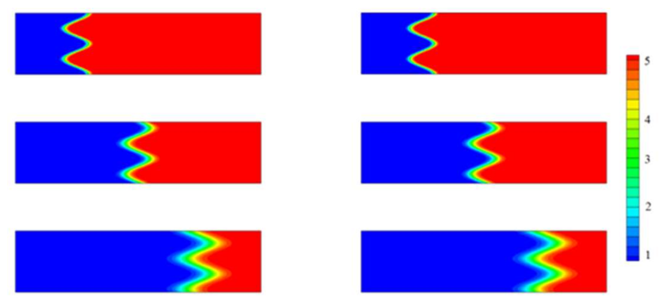
The two-dimensional case was simulated with different grids of 200 × 50, 400 × 100, 800 × 200, and 1600 × 400, while the time step was fixed as Δt = 0.00125. Under these conditions, the maximum Courant-Friedrichs-Lewy (CFL) numbers ranged from 0.15 to 1.2. The Dirichelet boundary condition was employed at x = −1, and the outlet boundary condition was applied at x = 3. The periodic boundary condition was employed at y = ±0.5. All of the tolerances for solving the linear equations in the CFD code were set to 10−10. The simulation results agreed well with the analytical solution, as shown in Figure 2.
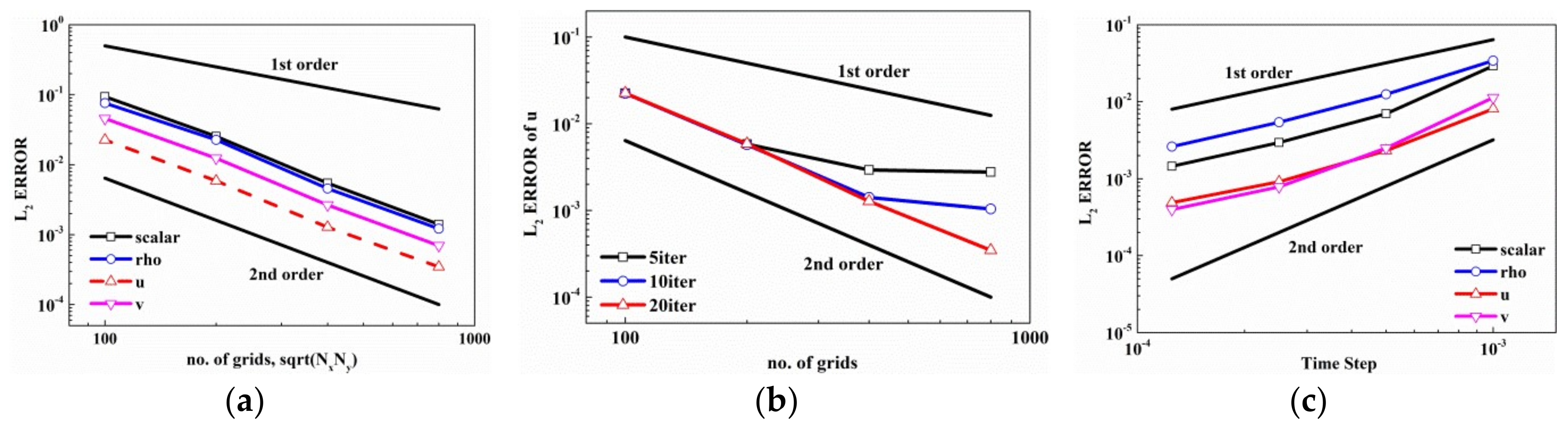
The maximum error (Lmax error) and volume-averaged error (L2 error) were typically employed to analyze the accuracy of the code in MMS analyses. If the overall order of accuracy of the code was second-order, the slope of the curves of the Lmax error and L2 error with different grid size would be two if plotted in a logarithmic coordinate. In the present study, we used the L2 error to determine the accuracy of our code, which was defined as the root mean square (R.M.S) between the simulation results and analytical results.
Figure 3a shows the spatial convergence of the L2 error of the scalar, u (velocity in x direction), v (velocity in y direction), and density when 20 sub-iterations were employed. It was found that all of the variables had a second-order accuracy.
To explore the effects of different sub-iteration numbers on the order of accuracy of the code, a series of cases with different numbers of sub-iterations per time step were employed. As shown in Figure 3b, the L2 error of u was significantly influenced by the sub-iteration number. When a fewer number of sub-iterations (<5) were used, the order of accuracy of the code tended to decrease to a first-order of accuracy, with more grid points being employed. On the other hand, as a larger number of sub-iterations (e.g., 20) were used, the order of accuracy of the code became more stable. It was also found that in the case with a relatively large density variance, a larger number of sub-iterations should have been used; otherwise the numerical results would diverge.
Figure 3c shows the convergence of the L2 error, with different sizes of the time step on the grid of 800 × 200, and only one sub-iteration per time step was applied. In theory, the L2 error should have come up with a first-order of accuracy; however the results showed that the order of accuracy was between one and two. It was caused by the relatively low density variance ratio (ρ0/ρ1 = 5) in this 2-D MMS case. Therefore, the code was able to achieve a higher order of accuracy with one sub-iteration.
3.2. A Sandia Turbuleut Non-Premixed Propane Jet
In this section, the code was used to simulate the turbulent non-premix propane jet experiment from the Sandia National Laboratory [42]. The nozzle of the jet was circular (with a diameter D = 52.6 mm) and was located in an air tube with a dimension of 30 cm × 30 cm. The mean velocity of the main jet velocity was 53 m/s and the measured maximum velocity at the centerline of the jet exit was 69 m/s. Therefore, the jet was regarded as a fully developed turbulent flow. The Rayleigh scattering was used for the density and propane mixture fraction measurements, while the velocity was measured by a two-color laser Doppler velocimetry (LDV) system. According to previous literature, the experimental uncertainties were as follows: mixture fraction Z = ±2%, Z′ = ±3%; velocity u = ±1%, v = ±1.5%, u′ = ±2%, v′ = ±2.5% (u is the X coordinate velocity and v is the Y coordinate velocity).
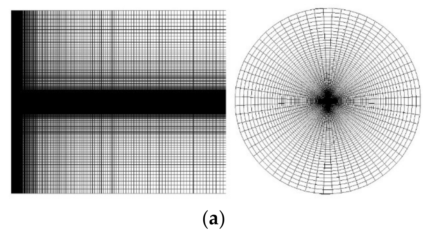
The computational grid was based on a cylindrical coordinate and the computational domain was 70D × 25D × 2π. The mesh had grid cells of 232 × 151 × 64 in the axial, radial, and azimuthal directions, respectively, and the total cell number was 2.24 million (shown in Figure 4a). Stretching grids were employed with a minimum cell size of 0.32 mm and a maximum size of 2.2 mm. The total computational time was about 30 flow-through times, the first 15 times were for the developing of the flow and the latter 15 times were for the purpose of the statistics. The inlet and outlet boundaries that were used here were mentioned above and the side boundaries were open-pressure boundaries.
The results of the major quantities along the centerline are shown in Figure 4b–d (x/D is the X coordinate value divided by nozzle diameter D). There were two different sets of experimental measurements of the velocity, based on where the LDV particles were seeded from (the main jet or the ambient air flow) [42]. As the results indicated, the simulation results agreed well with the experimental data. The under-prediction of the density for the simulation result was due to the numerical assumption or experimental errors at the inlet boundary. The better agreements between the simulation results and the experimental measurements demonstrated the capability of the present code for the large-eddy simulations of non-reacting turbulent flows.
3.3. Sandia Flame D
In previous literature, the Sandia Flames D–F were commonly employed in the validation of combustion models and reacting flow solvers [43]. This series of jet flames had an increasing jet velocity from Flame D to Flame F, which therefore exhibited an increasing level of local extinction, with Flame F being very close to blow-off. In this paper, only Flame D was applied as the validation case of our code for reacting turbulent flows. For Flame D [44], the burner had a central fuel nozzle with a diameter of D = 7.2 mm, and the main nozzle was surrounded by an annular nozzle with a diameter of 18.2 mm, which supported a pilot flame. The fuel injected from the main nozzle consisted of 25% CH4 and 75% air by volume, and the stoichiometric mixture fraction was Z = 0.351 (in Bilger’s definition). The pilot flame was a premixed flame, where the reactants had the same nominal enthalpy and equilibrium composition as CH4/air at the equivalence ratio of 0.77. The bulk velocity of the main jet was 49.7 m/s, and the pilot inlet velocity was set to 11.4 m/s.
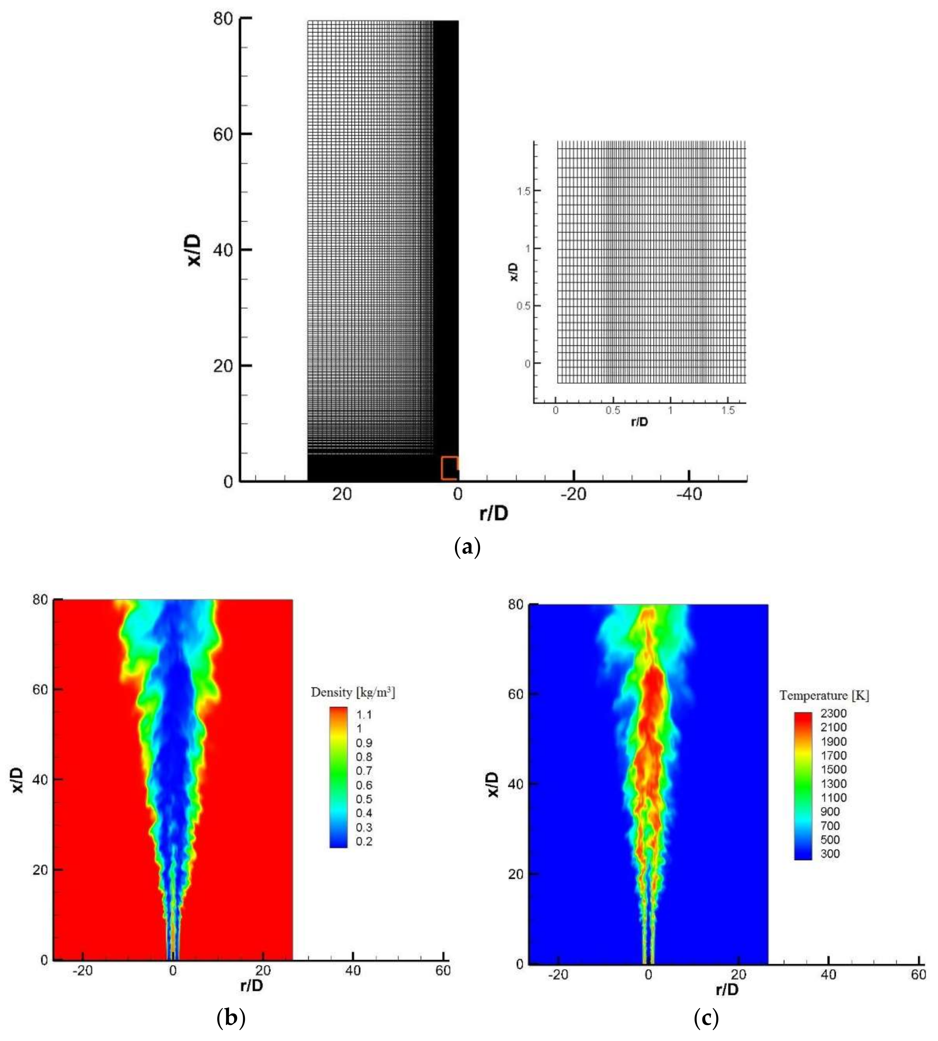
In the simulation, the flamelet/progress variable approach (FPV) was employed in our own code simulation. The computational domain employed a stretching grid with a dimension of 80D × 26.5D × 2π in the axial, radial, and azimuthal directions, respectively, and the corresponding grid cells were 256 × 160 × 64 (shown in Figure 5a). The smallest cells were located near the edge of the nozzle with a size of 0.25 mm × 0.25 mm × π/32 rad. The total computational time was about 20 flow-through times, with the later 10 times used for statistical purposes. The flamelet library was calculated using the FlameMaster, with the GRI 3.0 chemical mechanism containing 53 species and 325 reactions. The Lewis number was assumed to be unity and the effect of radiation was neglected as a simplification. The inlet and outlet boundaries that were used here were mentioned above and the side boundaries were open-pressure boundaries.
In contrast, a steady flamelet approach (SFA) [45], calculated by ANSYS Fluent with the same grid spacing, was also presented. The pressure-based solver, the large-eddy simulation turbulence model, and the steady flamelet model with the same GRI 3.0 mechanism were chosen in ANSYS Fluent (Version 18.0, ANSYS Inc., Canonsburg, PA 15317, USA). The inlet boundary conditions were handled by User Defined Function (UDF) with a turbulent intensity of 10%. The numerical scheme for the scalar transport equations was the QUICK scheme, while for all of the other equations it was the second-order upwind scheme.
The instantaneous view of the FPV results of the density and temperature are shown in Figure 5. As a result of the high temperature of the pilot, the main flame was directly anchored to the nozzle, which indicated that a pilot flame could be useful for combustion stabilization. The maximum temperature of the flame was about 2200 K, which was very close to the adiabatic flame temperature. It was reported that the visual flame length was about 67D (in the experiments, D is the nozzle diameter of 7.2 mm), which was almost the location where the maximum temperature was achieved in both FPV and SFA.
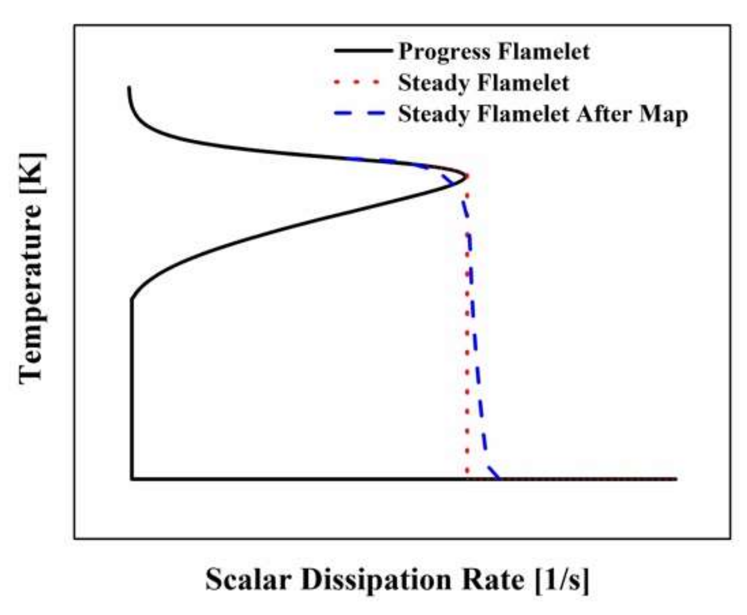
The comparisons between the experimental data and the simulation results are shown in Figure 6. It was found that the FPV results achieved a much better agreement with the experimental data than the SFA results. Compared with the experimental results and simulations, SFA under-predicted the decreasing of the velocity and the combustion rate, which resulted in a later occurrence of the peak of the temperature along the centerline. This was because of the lack of information in the steady flamelet table. During the LES simulation, the steady flamelet table was adjusted to avoid a breakpoint in the numerical calculation, which moved the critical point forward, as shown in Figure 7. Moving the critical point forward caused a delay on the prediction of combustion.
Figure 8 shows the comparisons between the simulation results and experimental data on species mass fractions, which were relevant to the combustion reaction. It was found that the peaks of all of the species mass fractions that were predicted by the SFA showed a later tendency of change than the FPV and experimental results, which could have been attributed to the under-estimation of the combustion reactions in the SFA. For the FPV, the simulation results on species mass fractions agreed with the experimental data better. Some minor over-prediction on intermediate species, such as CO, H2, and OH, might have been because of the slight over-estimation of the mixture fraction, which was also found in previous literature [46,47]. In summary, the FPV results were in an overall good agreement with the experimental data, which suggested that our LES code could predict turbulent reacting flows well.
4. Conclusions
In this study, a low-Mach-number LES code has been comprehensively verified and validated with analytical solutions and experimental measurements. The MMS approach employs manufactured source terms in the momentum and scalar transport equations, to simulate specified cases with analytical solutions. The simulation results are in good agreement with the analytical solutions. The spatial and temporal errors between them have been investigated, and the influence of the number of sub-iterations on the order of accuracy of the code have also been checked. In the validation with the Sandia propane jet and Flame D, the simulation results of the velocity, mixture fraction, temperature, and species mass fractions have been compared to the experiment data. The main conclusions are the following:
- The code has a second-order accuracy with a grid refinement in 2-D MMS verification.
- A proper sub-iteration number and tolerance of convergence should be used to ensure the order of accuracy.
- The LES code called ‘LESsCoal’ can give accurate predictions on non-reacting and reacting jet flow cases. The steady flamelet model tends to under-predict the combustion rate, because of the critical point moving forward in the steady flamelet table.
- The MMS method combined with some typical experimental results, which can give the order of accuracy and precision information about the code, is a useful verification and validation method.
The validated LES code can be used in our future LES investigations on the combustion of syngas produced from the gasification of coal and biomass. The fundamental turbulent combustion characteristics, for example, the flame temperature and lift-off height, can be obtained from the LES of jet flames. On the other hand, practical syngas combustors could also be numerically studied to improve their designs.
Acknowledgments
This work was supported by the National Natural Science Foundation of China (51706200, 51776185).
Author Contributions
Yingzu Liu, Kaidi Wan, and Liang Li designed and performed the simulations together; Zhihua Wang and Kefa Cen helped analyze the data and improve the simulations; all authors contributed to writing and revising the paper.
Conflicts of Interest
The authors declare no conflict of interest.
Nomenclature
| u | (m/s) | Velocity |
| t | (s) | Time |
| Sρ | (kg/m3·s) | Source term in continuity equation |
| Su | (kg/m2·s2) | Source term in momentum equation |
| SΦ | (kg/m3·s) | Source term in scalar transport equation |
| Φ | (-) | Scalar |
| Z | (-) | Mixture fraction |
| C | (-) | Reaction progress variable |
| p | (Pa) | Pressure |
| Y | (-) | Mass fraction |
| x | (m) | coordinate |
| y | (m) | coordinate |
| Q | varies | Unresolved part under SGS filter |
| T | (K) | Temperature |
| N | (-) | Number of variables for calculating the L2 error |
| L2 | (-) | L2 error |
| n | (m) | Boundary-normal coordinate |
| at | (-) | Turbulent diffusion coefficient |
| P | (-) | PDF function |
| c | (m/s) | Convection velocity |
| Z’ | (-) | Fluctuation of mixture fraction |
| u’ | (m/s) | Fluctuation of X coordination velocity |
| v’ | (m/s) | Fluctuation of Y coordination velocity |
| Greek symbols | ||
| ρ | kg/m3 | density |
| τij | (kg/m·s2) | Viscous stress tensor |
| σ | (-) | Kronecker delta |
| ωc | (kg/m3·s) | Chemical reaction source term in mass |
| χ | (1/s) | Scalar dissipation rate |
| αZ | (-) | Diffusivity of the scalar Z |
| αC | (-) | Diffusivity of the scalar C |
| Subscripts | ||
| i,j,k | Direction of the Cartesian coordinate | |
| Φ,sgs | Unresolved scalar flux | |
| sgs | Unresolved Reynold stress | |
| st | Stoichiometric | |
| sim | Simulation result | |
| ana | Analytical result | |
| Operators | ||
| Density-weighted spatial filtering | ||
| Spatial filtering | ||
| Sufficiently differentiable function | ||
References
- Wang, Z.; He, P.; Lv, Y.; Zhou, J.; Fan, J.; Cen, K. Direct numerical simulation of subsonic round turbulent jet. Flow Turbul. Combust. 2010, 84, 669–686. [Google Scholar] [CrossRef]
- Lee, D.; Huh, K.Y. DNS analysis of propagation speed and conditional statistics of turbulent premixed flame in a planar impinging jet. Proc. Combust. Inst. 2011, 33, 1301–1307. [Google Scholar] [CrossRef]
- Liu, T.; Bai, F.; Zhao, Z.; Lin, Y.; Du, Q.; Peng, Z. Large Eddy Simulation Analysis on Confined Swirling Flows in a Gas Turbine Swirl Burner. Energies 2017, 10, 2081. [Google Scholar] [CrossRef]
- Ciri, U.; Petrolo, G.; Salvetti, M.V.; Leonardi, S. Large-Eddy Simulations of Two In-Line Turbines in a Wind Tunnel with Different Inflow Conditions. Energies 2017, 10, 821. [Google Scholar] [CrossRef]
- Di Sarli, V.; Benedetto, A.D. Sensitivity to the presence of the combustion submodel for large eddy simulation of transient premixed flame–vortex interactions. Ind. Eng. Chem. Res. 2012, 51, 7704–7712. [Google Scholar] [CrossRef]
- Oberkampf, W.L.; Trucano, T.G. Verification and validation in computational fluid dynamics. Prog. Aeosp. Sci. 2002, 38, 209–272. [Google Scholar] [CrossRef]
- Eça, L.; Hoekstra, M.; Hay, A.; Pelletier, D. A manufactured solution for a two-dimensional steady wall-bounded incompressible turbulent flow. Int. J. Comput. Fluid Dyn. 2007, 21, 175–188. [Google Scholar] [CrossRef]
- Brady, P.; Herrmann, M.; Lopez, J. Code verification for finite volume multiphase scalar equations using the method of manufactured solutions. J. Comput. Phys. 2012, 231, 2924–2944. [Google Scholar] [CrossRef]
- Pitsch, H. Large-eddy simulation of turbulent combustion. Annu. Rev. Fluid Mech. 2006, 38, 453–482. [Google Scholar] [CrossRef]
- Le Clainche, S.; Ferrer, E. A Reduced Order Model to Predict Transient Flows around Straight Bladed Vertical Axis Wind Turbines. Energies 2018, 11, 566. [Google Scholar] [CrossRef]
- Colucci, P.; Jaberi, F.; Givi, P.; Pope, S. Filtered density function for large eddy simulation of turbulent reacting flows. Phys. Fluids 1998, 10, 499–515. [Google Scholar] [CrossRef]
- Navarro-Martinez, S.; Kronenburg, A.; Di Mare, F. Conditional moment closure for large eddy simulations. Flow Turbul. Combust. 2005, 75, 245–274. [Google Scholar] [CrossRef]
- Ihme, M.; Pitsch, H. Prediction of extinction and reignition in nonpremixed turbulent flames using a flamelet/progress variable model: 2. Application in LES of Sandia flames D and E. Combust. Flame 2008, 155, 90–107. [Google Scholar] [CrossRef]
- Hawkes, E.; Cant, R. A flame surface density approach to large-eddy simulation of premixed turbulent combustion. Proc. Combust. Inst. 2000, 28, 51–58. [Google Scholar] [CrossRef]
- Chakravarthy, V.; Menon, S. Large-eddy simulation of turbulent premixed flames in the flamelet regime. Combust. Sci. Technol. 2001, 162, 175–222. [Google Scholar] [CrossRef]
- Pitsch, H.; De Lageneste, L.D. Large-eddy simulation of premixed turbulent combustion using a level-set approach. Proc. Combust. Inst. 2002, 29, 2001–2008. [Google Scholar] [CrossRef]
- Park, T.S. LES and RANS simulations of cryogenic liquid nitrogen jets. J. Supercrit. Fluids 2012, 72, 232–247. [Google Scholar] [CrossRef]
- Ozawa, T.; Lesbros, S.; Hong, G. LES of synthetic jets in boundary layer with laminar separation caused by adverse pressure gradient. Comput. Fluids 2010, 39, 845–858. [Google Scholar] [CrossRef]
- Bonelli, F.; Viggiano, A.; Magi, V. How does a high density ratio affect the near-and intermediate-field of high-Re hydrogen jets? Int. J. Hydrogen Energy 2016, 41, 15007–15025. [Google Scholar] [CrossRef]
- Chen, Z.; Ruan, S.; Swaminathan, N. Large Eddy Simulation of flame edge evolution in a spark-ignited methane-air jet. Proc. Combust. Inst. 2017, 36, 1645–1652. [Google Scholar] [CrossRef]
- Gicquel, L.Y.; Staffelbach, G.; Poinsot, T. Large Eddy Simulations of gaseous flames in gas turbine combustion chambers. Prog. Energy Combust. Sci. 2012, 38, 782–817. [Google Scholar] [CrossRef] [Green Version]
- Klein, R. Semi-implicit extension of a Godunov-type scheme based on low Mach number asymptotics I: One-dimensional flow. J. Comput. Phys. 1995, 121, 213–237. [Google Scholar] [CrossRef]
- Majda, A.; Sethian, J. The derivation and numerical solution of the equations for zero Mach number combustion. Combust. Sci. Technol. 1985, 42, 185–205. [Google Scholar] [CrossRef]
- Vedovoto, J.M.; da Silveira Neto, A.; Mura, A.; da Silva, L.F.F. Application of the method of manufactured solutions to the verification of a pressure-based finite-volume numerical scheme. Comput. Fluids 2011, 51, 85–99. [Google Scholar] [CrossRef]
- Germano, M.; Piomelli, U.; Moin, P.; Cabot, W.H. A dynamic subgrid-scale eddy viscosity model. Phys. Fluids 1991, 3, 1760–1765. [Google Scholar] [CrossRef]
- Lilleberg, B.; Panjwani, B.; Ertesvåg, I.S. Large Eddy Simulation of Methane Diffusion Flame: Comparison of Chemical Kinetics Mechanisms. AIP Conf. Proc. 2010, 1281, 2158–2161. [Google Scholar]
- Sheikhi, M.; Drozda, T.; Givi, P.; Jaberi, F.; Pope, S. Large eddy simulation of a turbulent nonpremixed piloted methane jet flame (Sandia Flame D). Proc. Combust. Inst. 2005, 30, 549–556. [Google Scholar] [CrossRef]
- Pierce, C.D.; Moin, P. Progress-variable approach for large-eddy simulation of non-premixed turbulent combustion. J. Fluid Mech. 2004, 504, 73–97. [Google Scholar] [CrossRef]
- Wall, C.; Pierce, C.D.; Moin, P. A semi-implicit method for resolution of acoustic waves in low Mach number flows. J. Comput. Phys. 2002, 181, 545–563. [Google Scholar] [CrossRef]
- Shunn, L.; Ham, F. Method of Manufactured Solutions Applied to Variable-Density Flow Solvers; Annual Research Briefs, Center for Tubluence Research: Stanford, CA, USA, 2007; pp. 155–168. [Google Scholar]
- Saad, Y.; Schultz, M.H. GMRES: A generalized minimal residual algorithm for solving nonsymmetric linear systems. SIAM J. Sci. Comput. 1986, 7, 856–869. [Google Scholar] [CrossRef]
- Bunch, J.R.; Hopcroft, J.E. Triangular factorization and inversion by fast matrix multiplication. Math. Comput. 1974, 28, 231–236. [Google Scholar] [CrossRef]
- Leonard, B.P. A stable and accurate convective modelling procedure based on quadratic upstream interpolation. Comput. Meth. Appl. Mech. Eng. 1979, 19, 59–98. [Google Scholar] [CrossRef]
- Morinishi, Y.; Vasilyev, O.V.; Ogi, T. Fully conservative finite difference scheme in cylindrical coordinates for incompressible flow simulations. J. Comput. Phys. 2004, 197, 686–710. [Google Scholar] [CrossRef]
- Ihme, M.; Shunn, L.; Zhang, J. Regularization of reaction progress variable for application to flamelet-based combustion models. J. Comput. Phys. 2012, 231, 7715–7721. [Google Scholar] [CrossRef]
- Pitsch, H.; Ihme, M. An unsteady/flamelet progress variable method for LES of nonpremixed turbulent combustion. In Proceedings of the 43rd AIAA Aerospace Sciences Meeting and Exhibit, Reno, Nevada, 10–13 January 2005. [Google Scholar]
- Ihme, M.; Pitsch, H. LES of a non-premixed flame using an extended flamelet/progress variable model. In Proceedings of the 43rd AIAA Aerospace Sciences Meeting, Reno, Nevada, 10–13 January 2005. [Google Scholar]
- Pierce, C.D.; Moin, P. Method for generating equilibrium swirling inflow conditions. AIAA J. 1998, 36, 1325–1327. [Google Scholar] [CrossRef]
- Bell, J.B.; Marcus, D.L. A second-order projection method for variable-density flows. J. Comput. Phys. 1992, 101, 334–348. [Google Scholar] [CrossRef]
- Forestier, M.; Pasquetti, R.; Peyret, R.; Sabbah, C. Spatial development of wakes using a spectral multi-domain method. Appl. Numer. Math. 2000, 33, 207–216. [Google Scholar] [CrossRef]
- Shunn, L.; Ham, F.; Moin, P. Verification of variable-density flow solvers using manufactured solutions. J. Comput. Phys. 2012, 231, 3801–3827. [Google Scholar] [CrossRef]
- Schefer, R.; Hartmann, V.; Dibble, R. Conditional sampling of velocity in a turbulent nonpremixed propane jet. AIAA J. 1987, 25, 1318–1330. [Google Scholar] [CrossRef]
- Pitsch, H.; Steiner, H. Large-eddy simulation of a turbulent piloted methane/air diffusion flame (Sandia flame D). Phys. Fluids 2000, 12, 2541–2554. [Google Scholar] [CrossRef]
- Barlow, R.; Karpetis, A. Measurements of scalar variance, scalar dissipation, and length scales in turbulent piloted methane/air jet flames. Flow Turbul. Combust. 2004, 72, 427–448. [Google Scholar] [CrossRef]
- Minotti, A.; Sciubba, E. LES of a meso combustion chamber with a detailed chemistry model: Comparison between the flamelet and EDC models. Energies 2010, 3, 1943–1959. [Google Scholar] [CrossRef]
- Jones, W.; Prasad, V. Large Eddy Simulation of the Sandia Flame Series (D–F) using the Eulerian stochastic field method. Combust. Flame 2010, 157, 1621–1636. [Google Scholar] [CrossRef]
- Vreman, A.; Albrecht, B.; Van Oijen, J.; De Goey, L.; Bastiaans, R. Premixed and nonpremixed generated manifolds in large-eddy simulation of Sandia flame D and F. Combust. Flame 2008, 153, 394–416. [Google Scholar] [CrossRef]
Figure 1.
The locus of the maximum temperature and maximum progress variable C from a complete flamelet library (including the unstable branch).
Figure 1.
The locus of the maximum temperature and maximum progress variable C from a complete flamelet library (including the unstable branch).

Figure 2.
Two-dimensional (2-D) manufactured solutions of density at different times (top: t = 0.0, middle: t = 0.5, and bottom: t = 1.0), left: analytical solution, right: numerical results of the code.
Figure 2.
Two-dimensional (2-D) manufactured solutions of density at different times (top: t = 0.0, middle: t = 0.5, and bottom: t = 1.0), left: analytical solution, right: numerical results of the code.

Figure 3.
2-D manufactured solutions: L2 error: (a) L2 error at t = 1 with grid refinement; (b) L2 error of u at t = 1 for different numbers of sub-iteration; and (c) L2 error at t = 0.1 using 1 sub-iteration on 800 × 200 grids (u—velocity in x direction; v—velocity in y direction).
Figure 3.
2-D manufactured solutions: L2 error: (a) L2 error at t = 1 with grid refinement; (b) L2 error of u at t = 1 for different numbers of sub-iteration; and (c) L2 error at t = 0.1 using 1 sub-iteration on 800 × 200 grids (u—velocity in x direction; v—velocity in y direction).

Figure 4.
(a) Computational grid and simulation results of the major quantities along the centerline: (b) velocity of u; (c) mixture fraction; and (d) density.
Figure 4.
(a) Computational grid and simulation results of the major quantities along the centerline: (b) velocity of u; (c) mixture fraction; and (d) density.


Figure 5.
(a) Computational grid and (b) instantaneous view of the density, and (c) instantaneous view of the temperature.
Figure 5.
(a) Computational grid and (b) instantaneous view of the density, and (c) instantaneous view of the temperature.

Figure 6.
Comparison of key variables along the centerline (SFA—steady flamelet approach; FPV—flamelet/progress variable; R.M.S—root mean square).
Figure 6.
Comparison of key variables along the centerline (SFA—steady flamelet approach; FPV—flamelet/progress variable; R.M.S—root mean square).

Figure 7.
Schematic diagram of the comparison between the progress flamelet and steady flamelet.

Figure 8.
Favre-averaged species mass fractions along the centerline.


Table 1.
Parameters and values for the 2-D case.
| Parameter | Value | Parameter | Value |
|---|---|---|---|
| ρ0 | 5 | a | 0.2 |
| ρ1 | 1 | b | 20 |
| uf | 2 | k | 4π |
| vf | 0.8 | w | 1.5 |
| 0.001 | 0.001 |
© 2018 by the authors. Licensee MDPI, Basel, Switzerland. This article is an open access article distributed under the terms and conditions of the Creative Commons Attribution (CC BY) license (http://creativecommons.org/licenses/by/4.0/).
Share and Cite
MDPI and ACS Style
Liu, Y.; Wan, K.; Li, L.; Wang, Z.; Cen, K. Verification and Validation of a Low-Mach-Number Large-Eddy Simulation Code against Manufactured Solutions and Experimental Results. Energies 2018, 11, 921. https://doi.org/10.3390/en11040921
AMA Style
Liu Y, Wan K, Li L, Wang Z, Cen K. Verification and Validation of a Low-Mach-Number Large-Eddy Simulation Code against Manufactured Solutions and Experimental Results. Energies. 2018; 11(4):921. https://doi.org/10.3390/en11040921
Chicago/Turabian StyleLiu, Yingzu, Kaidi Wan, Liang Li, Zhihua Wang, and Kefa Cen. 2018. "Verification and Validation of a Low-Mach-Number Large-Eddy Simulation Code against Manufactured Solutions and Experimental Results" Energies 11, no. 4: 921. https://doi.org/10.3390/en11040921
Note that from the first issue of 2016, this journal uses article numbers instead of page numbers. See further details here.