DC Fault Analysis and Clearance Solutions of MMC-HVDC Systems


College of Electrical Engineering, Zhejiang University, Hangzhou 310027, China
*
Author to whom correspondence should be addressed.
Energies 2018, 11(4), 941; https://doi.org/10.3390/en11040941
Submission received: 18 March 2018
/
Revised: 11 April 2018
/
Accepted: 13 April 2018
/
Published: 16 April 2018
(This article belongs to the Section F: Electrical Engineering)
Abstract
:In this paper, the DC short-circuit fault and corresponding clearance solutions of modular multilevel converter-based high-voltage direct current (MMC-HVDC) systems are analyzed in detail. Firstly, the analytical expressions of DC fault currents before and after blocking the MMC are derived based on the operation circuits. Before blocking the MMC, the sub-module (SM) capacitor discharge current is the dominant component of the DC fault current. It will reach the blocking threshold value in several milliseconds. After blocking the MMC, the SM capacitor is no longer discharged. Therefore, the fault current from the AC system becomes the dominant component. Meanwhile, three DC fault clearance solutions and the corresponding characteristics are discussed in detail, including tripping AC circuit breaker, adopting the full-bridge MMC and employing the DC circuit breaker. A simulation model of the MMC-HVDC is realized in PSCAD/EMTDC and the results of the proposed analytical expressions are compared with those of the simulation. The results show that the analytical DC fault currents coincide well with the simulation results.
1. Introduction
With the growth of energy demand and the gradual exhaustion of fossil fuels, the development and integration of renewable energy sources has become increasingly important in recent years. According to practical experience, voltage source converter-based high-voltage direct current (VSC-HVDC) systems are considered to be one of the best solutions for renewable energy integration [1,2].
The modular multilevel converter (MMC) is considered to be the most promising VSC topology [3,4,5]. Because of the modular construction, the series connection of power electronic devices is avoided. So the difficulty in manufacturing is reduced [6,7,8]. The MMC-HVDC system can provide excellent outputs of modulated voltage and current, and has been widely used in commercial projects [9,10,11].
Up till now, a lot of studies have been focused on the modeling [12,13,14], control [15,16,17] and steady-state analysis [18,19] of the MMC-HVDC. When the MMC is used in long-distance overhead line transmissions or DC grids, the DC fault characteristics and the corresponding clearance solutions should be analyzed in depth. A mathematical model of two-terminal VSC-HVDC under various DC fault conditions is built in [20]. In [21], theoretical analysis of VSC cable fault with three stages is proposed. However, both [20,21] are based on two-level converters. The performance of MMC under pole-to-ground fault is analyzed and expression for DC current is derived in [22]. However, the equivalent DC voltage is achieved with the conventional half-wave rectifier bridge. It should be noted that the equivalent circuit after blocking the MMC is different from the conventional half-wave rectifier bridge, as the former one has an inductor in each arm. A pole-to-pole fault analysis of multi-terminal MMC systems is proposed in [23]. However, the fault current is obtained by electromagnetic transient simulations. Analytical fault current calculation method of pole-to-pole fault for one terminal MMC and MMC-based DC grids are introduced in [24,25]. However, the fault current expressions are valid only before blocking the MMC. Reference [26] derives the detailed differential equations of MMC in both pre-blocking and post-blocking conditions, and also proposes the corresponding solving method. However, this method belongs to numerical analysis and the analytical solution cannot be given.
DC fault isolation is the most important technical obstacle that limits the application of MMC in long-distance overhead line transmissions or DC grids. Generally, there have been three solutions for solving this problem [27,28]:
- The first solution is to trip the AC circuit breaker (ACCB). The advantages of this method are the good economic efficiency and the high technical maturity. That is the reason most practical commercial VSC-HVDC projects use this method to clear DC line faults. Noted the slow response of the ACCB, it will take a long time for the system to recover from the DC line faults [27].
- Adopting fault blocking converters is another option [29]. To prevent IGBT damage due to overheating, converters will be blocked when the current flowing through the IGBT reaches 2 times of its rated value. Some converters may produce reversed electromotive force to impede the fault current, such as full-bridge MMC. For this solution, the speed of resuming power transmission from temporary DC faults is fast. However, more power electronic devices are needed, and the device cost and power losses increase accordingly. Compared with the half-bridge sub-modules (SMs) MMC, the converter based on full-bridge SMs needs twice insulated gate bipolar transistor (IGBT) modules and the power losses increase by about 100%; the converter based on clamp-double SMs needs 1.25 times IGBT modules and the power losses increase by about 35% [30].
- The employing of DC circuit breakers (DCCBs) is the third method for handling DC fault. In late 2012, ABB released a hybrid DCCB that can break a maximum DC fault current of 9 kA within 5 ms [31]. Technically speaking, there have been some drawbacks for the existing DCCBs, such as high manufacture cost and low technology maturity.
Moreover, the fault recovery characteristics of the MMC with the above three solutions are not analyzed in detail.
In this paper, the analytical expressions of DC currents under pole-to-pole fault are derived and the fault characteristics of the MMC with different solutions are analyzed. Firstly, the analytical DC fault current expression of MMC before blocking is derived based on the operation circuit in complex frequency domain. Secondly, after the MMC is blocked, the DC current expression is also derived. Besides, three DC fault clearance solutions and the corresponding characteristics are discussed in detail.
This paper is organized as follows. The analytical expressions of the fault currents before and after blocking the MMC are studied in Section 2 and Section 3 respectively. In Section 4 the three DC fault clearance solutions are discussed. In Section 5, an MMC-HVDC model is built in PSCAD/EMTDC to verify the accuracy and feasibility of the proposed analytical expressions. Section 6 concludes the paper.
2. DC Fault Analysis of MMC before Blocking
Figure 1 shows the DC short-circuit fault of MMC. The arm voltage and the arm current are urj (r = p, n denotes the upper and lower arms; j = a, b, c denotes the three phases a, b, c) and irj respectively. Udc is the DC voltage and Idc is the DC line current. The fault current mainly contains the SM capacitor discharge current and three-phase short-circuit current of the AC system. Before blocking the MMC, the SM capacitor discharge current is the dominant component. The fault current rises so fast that it can reach several tens of kA in a few milliseconds.
In this stage, the number of inserted SMs in each arm changes constantly. This is a nonlinear time-varying circuit. However, if the period of the analysis is sufficiently short that the inserted SMs remain unchanged, then the MMC is a linear circuit during this period.
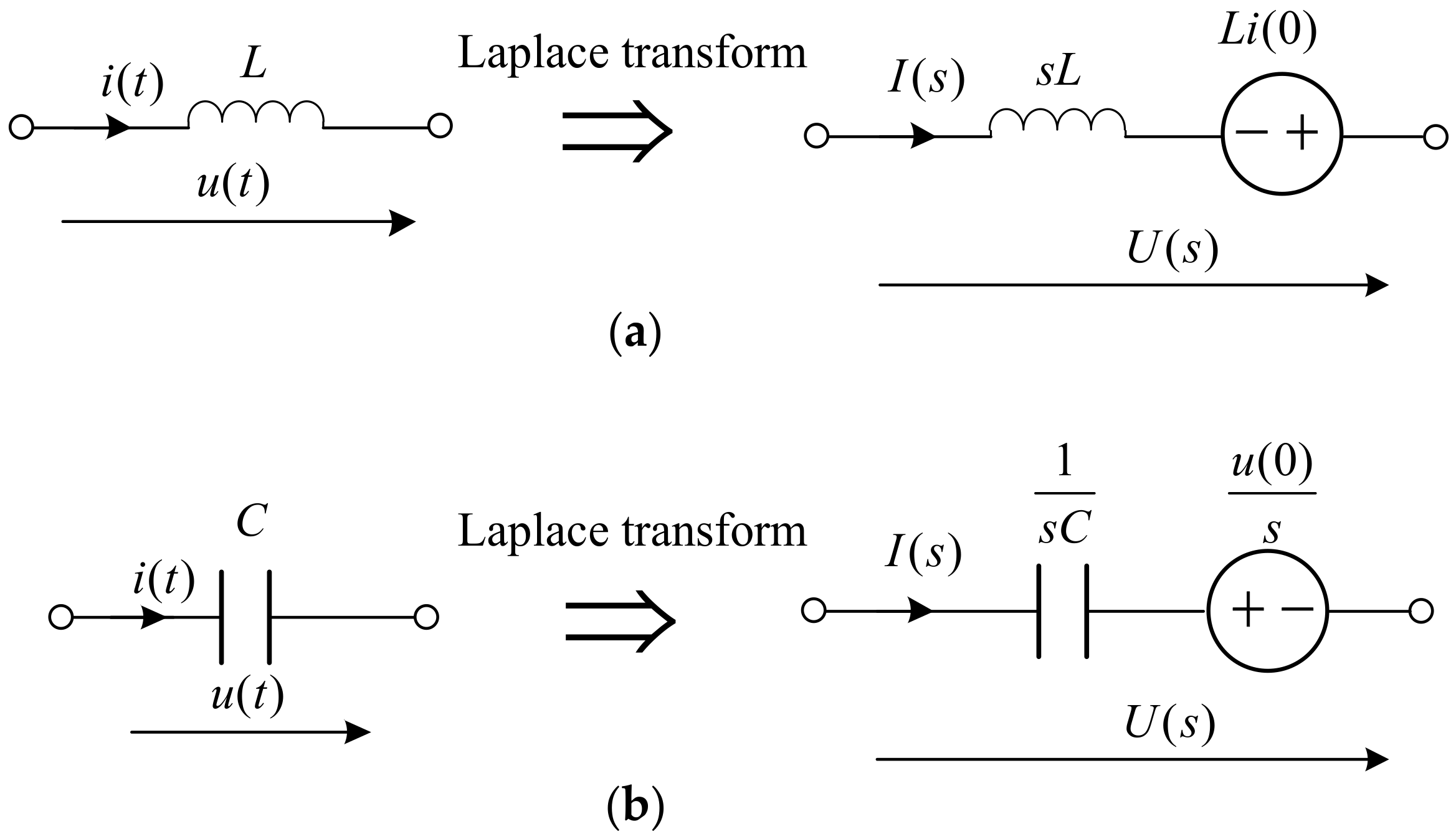
The operation circuit analysis (also called complex frequency domain analysis) is an effective method to analyze the transient process of a linear circuit. The specific approach is to replace the impedance and admittance with operational impedance and operational admittance respectively. The inductor and capacitor operation circuit model is shown in Figure 2. sL and 1/sC are their operation impedances, where s is the Laplace operator. Appendix A shows the detailed derivation.
The complete operation circuit of Figure 1 is depicted in Figure 3a. Rdc and Ldc include the resistance and inductance of smoothing reactor, DC circuit breaker and DC line. R0 represents the loss of each arm. C0 is the SM capacitance. N is the number of SMs in each arm. In the three-phase symmetrical system, the sum of AC system three-phase short-circuit current is zero. Also, as mentioned above, the SM capacitor discharge current is the dominant fault current before blocking the MMC. Therefore, the part of AC system can be ignored here. In this way, Figure 3a can be simplified to Figure 3b. Figure 3c is the equivalent circuit of Figure 3b. It should be noted that the quantities marked zero (i.e., idc(0), upc(0), ic(0), …) are their initial values before the fault occurs.
Solving the simplified circuit shown in Figure 3c, the following equation can be obtained
The Laplace inverse transform of (1) yields
where idc(0) is the initial DC current, and
3. DC Fault Analysis of MMC after Blocking
After blocking the MMC, the SM capacitor is no longer discharged. Therefore, the fault current from the AC system becomes the dominant component. Figure 4 shows the equivalent circuit of the MMC after it is blocked. The quantities marked with ‘∞’ (i.e., ia∞, ipa∞, Idc∞,…) are their steady state value. To simplify the analysis, short-circuit fault located at the outlet of the smoothing reactor is considered. In this way, the positive common point Bp and negative common point Bn are equipotential. Due to the symmetry of the diode rectifier circuit, it can be considered that point O’ is also equipotential with Bp and Bn.
Take phase a as the example, the AC voltage is given by
According to the MMC operation principle [18], the upper and lower arm currents can be expressed as
where A0 and An are DC component and nth harmonic component of the arm current. Based on the relation between arm current and output current [14], the expression of output current ia∞ can be written as
where k is the positive integer.
Applying Kirchhoff’s voltage law (KVL) to phase a of Figure 4 yields
In (10) R0 is ignored because it is very small; and it is considered that point O’ is equipotential with Bp and Bn.
Inserting (7)–(9) to (10), the following expression is obtained
Comparing the left side and right side of (11), we know
Therefore, the arm current is rewritten as
Two characteristics of the diode rectifier circuit shown in Figure 4 are used to determine the value of A0. The first characteristic is the unidirectional conductivity of the diode valve, which means ipa∞ (t) ≥ 0. So, we have
The second characteristic is the presence of multiple zeroes in the diode valve current. In fact, for the diode rectifier circuit shown in Figure 4, when R0 is considered, there exists a certain period of time that the arm current ipa∞ (t) equals zero in each fundamental frequency cycle. Thus, we know
According to (16) and (17), the value of A0 is given by
In this way, the arm current expression is
Then the steady-state DC fault current can be expressed as
It should be noted that, the expression shown in (20) is the steady-state value after blocking the MMC. It takes a certain amount of time for DC current varying from the moment of blocking to the steady state. This process can generally be described by a first-order inertia process. If we redefine the time starting point as the MMC blocking moment, the complete DC current expression can be given by
where IdcB is the initial DC current after MMC is blocked. τdcB is the first-order inertia time constant, the value of which is closely related to the inductance of the smoothing reactor. For the practical project, τdcB is between 10 ms and 200 ms.
4. Three DC Fault Clearance Solutions and Corresponding Characteristics
In this section, three DC fault clearance solutions are presented, including (1) tripping the AC circuit breaker; (2) adopting the full-bridge SM-based MMC (F-MMC) and (3) employing the DC circuit breaker. Besides, the DC fault characteristics of these three solutions are analyzed in detail.
4.1. Solution 1: Tripping AC Circuit Breaker
Tripping AC circuit breakers (ACCB) is a straightforward solution to clear DC faults for the MMC-HVDC. The DC fault clearance process can be divided into three states as follows.
State 1: Fault detection and DC blocking. After DC fault occurs, the DC current rises sharply. When the fault is detected, all the IGBTs of the MMC will be blocked. In this state the DC fault characteristics are the same as that presented in Section 2.
State 2: Trip the AC circuit breaker. After blocking the MMC, the tripping signal is sent to the ACCB. However, the response of the ACCB is slow, which requires about 60–100 ms. In this state the DC fault characteristics have been presented in Section 3.
State 3: Fault arc extinguishment. After the ACCB is tripped, the residual DC fault currents will gradually decay through the damping loop shown in Figure 5a. The operation circuit of Figure 5a is illustrated in Figure 5b. Solving the operation circuit, the following equation can be obtained
where IdcT is the DC current at the moment when the ACCB is tripped. The Laplace inverse transform of (22) yields
where the decay time constant is
When the residual DC fault current is less than the DC breaking current of the DC pole switch, the DC pole switch can then be tripped. However, as the decay time constant in (24) is large (more than 5 s), it may take a long time for the fault current to decrease to the threshold value.
4.2. Solution 2: Adopting F-MMC with DC Fault Clearance Capability
Adopting converters with DC fault clearance capability is another alternative. The F-MMC is considered in this paper. The DC fault clearance process contains two states as follows.
State 1: Fault detection and DC blocking. When the fault is detected, all the IGBTs of the F-MMC will be blocked. Before blocking, the fault characteristics of the F-MMC are the same as that of the H-MMC proposed in Section 2.
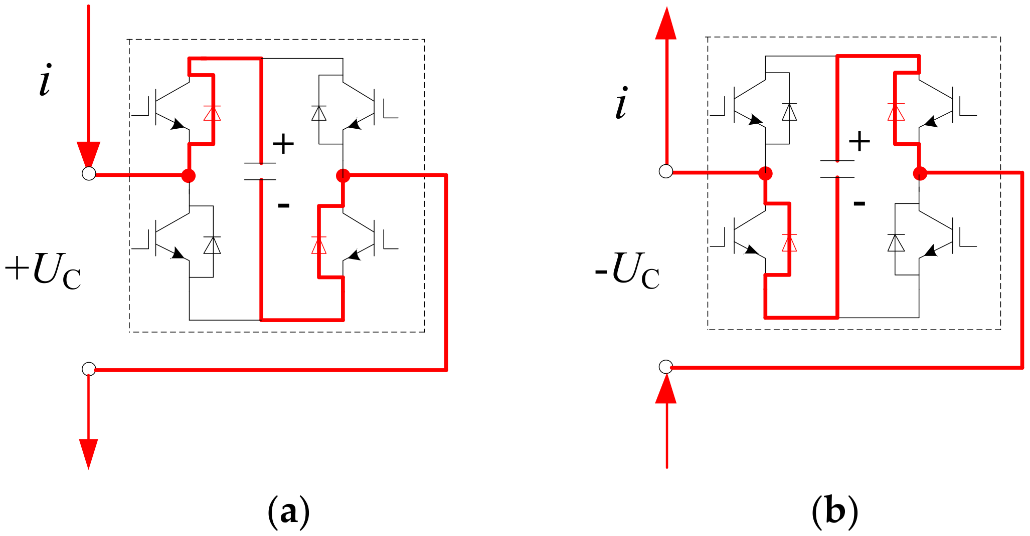
State 2: Fast fault arc extinguishment. After the F-MMC is blocked, the current path in a full-bridge SM (FBSM) is shown in Figure 6. The back electromotive forces (EMFs) provided by the blocked FBSMs will impede the AC feeding current. The equivalent circuit of the system is depicted in Figure 7a. Figure 7b shows its operation circuit. The DC current can be given by solving the operation circuit
where IdcB and UdcB are the initial DC current and DC voltage after blocking the F-MMC. The Laplace inverse transform of (25) yields
where
4.3. Solution 3: Adopting DC Circuit Breaker
The third method to clear DC fault is employing the DC circuit breaker (DCCB). The hybrid DCCB proposed in [31] is used in this paper, whose basic structure is shown in Figure 8. This DCCB consists of a normal path and a fault path in parallel. In the normal path, a semiconductor-based load commutation switch (LCS) is in series with an ultra-fast disconnector (UFD). The fault path is formed by a main circuit breaker (MB). The procedure of isolating faulty lines is as follows:
State 1: Fault detection. This state is the same as that proposed in Section 2.
State 2: Trip the DC circuit breaker. When a DC fault is detected, the LCS will open immediately and the current will be commutated to the MB. Then the UFD will open within 2 ms and isolate the LCS from the faulted line. With the UFD in open position, the MB will break the current. Finally, the remaining energy is consumed by the arrester banks. In fact, from the start action of the DCCB to MB breaks the current, the MMC still operates in the state presented in Section 2. This process lasts about 2.3 ms. After that, the DC current will decrease quickly due to the access of the arrester. Assume that the DC fault current decreases linearly to zero in a short time ∆t. The expression of the current can be given by
where IdcT2 is the initial DC current when MB is switched off.
5. Case Study
5.1. Test System
To verify the accuracy and effectiveness of the analytical expressions derived in this paper, an MMC test system shown in Figure 9 is built in PSCAD/EMTDC. The main circuit parameters are listed in Table 1. In steady state, the MMC is operated with constant active power control and constant reactive power control. The reference values are 400 MW and 0 Mvar respectively.
5.2. Performances of MMC Before Blocking
The system operates in steady state before the fault occurs. At t = 2 s, a DC fault is applied to the DC side outlet of the MMC. Figure 10 shows the simulation result and the analytical result of the DC current. The fault current increases sharply after the DC fault. In 5 ms the fault current rises from 1 kA to over 8 kA. The results also show that the analytical result agrees well with the simulation one.
It is a fact that the MMC will be blocked when the arm currents reach two times of IGBT rated value. Figure 11 illustrates the maximum current of the six arms. For this test system the rated current of the IGBT is 1.5 kA. Therefore, the MMC will be blocked at t = 2.00356 s as the arm current reaches 3.0 kA.
5.3. Performances of MMC after Blocking
A DC fault occurs at t = 2 s, and the MMC is blocked at t = 2.00356 s. The DC currents obtained from the simulation and analytical expression (21) are shown in Figure 12. The two results are consistent with each other, and the error between them is very small. After blocking the MMC, the DC fault current increases to a steady value gradually. In addition, the steady-state DC fault current is about 11.5 kA.
5.4. Performances of MMC with Solution 1
A DC fault occurs at t = 2 s, and the MMC is blocked at t = 2.00356 s. Considering the slow response of the AC circuit breaker, it is tripped at t = 2.06 s. The results are illustrated in Figure 13. The fault current goes down in a very slow speed. It takes about 9258 ms for the fault current reduce to near zero (for example 200 A). The results show a strong agreement between the simulation and the analysis.
5.5. Performances of MMC with Solution 2
In this case, the half-bridge SMs are replaced with full-bridge SMs, and the rest parts of the system remain unchanged. A DC fault occurs to the system at t = 2 s, and the F-MMC is blocked at t = 2.00356 s. Figure 14 shows the corresponding DC fault currents. It can be seen that there is some difference between the simulation result and the analytical result. The main reason is that the analytical expression given by (26) neglects the impact of the AC system. In fact, the AC voltage has influence to the decrease of the DC fault current, especially when the DC voltage is smaller than the amplitude of the AC phase voltage. The fault current reduces to zero in about 2.16 ms.
If the F-MMC is blocked and the ACCB is tripped at the same time, the AC system has no influence on the DC current. In addition, the corresponding fault currents given by simulation and analytical expression are shown in Figure 15. The results show that the results obtained by the two methods are consistent.
5.6. Performances of MMC with Solution 3
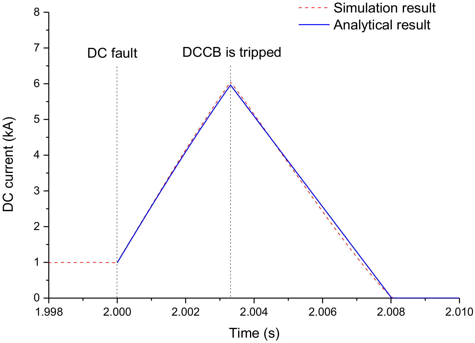
At t = 2 s, a DC fault occurs at the DC side outlet of the MMC. The relay system completes the fault location detection in 1 ms, and a turn-off signal is sent to the LCS of the DCCB. At t = 2.00125 s the LCS is opened and the UFD starts action. At t = 2.0033 s the UFD is switched off and the MB is activated. Then the fault current will decrease quickly to zero due to the access of the arrester at t = 2.00806 s. The DC fault currents are shown in Figure 16. As the faulty line is isolated at t = 2.0033 s, the maximum arm current is less than the blocking threshold value. Therefore, the MMC will not be blocked. From the figure it can be seen that the analytical result agrees well with the simulation result, which proves the accuracy of the analytical expressions.
5.7. Comparison of Three Solutions
Three key quantities of the system with different DC fault clearance solutions are list in Table 2, including the fault clearance time and the maximum fault current. It is seen that Solution 1 has the longest fault clearance time and the largest maximum fault current. Compared with Solution 2, the fault clearance time of Solution 3 is slightly larger but the maximum fault current is smaller. Among the three solutions, the converters under Solution 3 will not be blocked, which means the power can be continuously transmitted when a DC fault occurs in MMC-based DC grids.
6. Conclusions
This paper analyzes the DC short-circuit fault of the MMC. By operation circuit in complex frequency domain, the analytical DC current expressions of the MMC under short-circuit fault are derived. Before the MMC is blocked, the DC fault current increases sharply and will reach the blocking threshold value in several milliseconds. After the MMC is blocked, the DC fault current will increase to the steady-state value gradually. Three DC fault clearance solutions and their characteristics are discussed in detail. Among these solutions, the fault clearance time of adopting F-MMC is the fastest. The solution of employing DC circuit breaker has the smallest maximum fault current, and the converters will not be blocked during fault period. An MMC model is developed in PSCAD/EMTDC, and the simulation results prove the accuracy and the feasibility of the proposed analytical expressions.
Acknowledgments
This paper is supported by the Headquarters Research Projects of State Grid Corporation of China “Research on superconducting DC fault current limiter and its coordination with DC circuit breaker (SGTYHT/17-JS-199)”.
Author Contributions
Zheng Xu proposed the kernel of the method; Huangqing Xiao derived the expressions and performed the simulations; Huangqing Xiao, Liang Xiao and Zheren Zhang wrote the paper.
Conflicts of Interest
The authors declare no conflict of interest.
Appendix A
The detailed derivation of inductor and capacitor operation circuit models are shown in this appendix. As for an inductor shown in the left side of Figure 2a, the voltage equation can be given by
Applying Laplace transformation to (A1) yields
From (A2) the inductor operation circuit is obtained in the right side of Figure 2a.
Similarly, as for a capacitor shown in the left side of Figure 2b, the current equation is given by
Applying Laplace transformation to (A3) yields
Solving (A4), the capacitor voltage can be expressed as
From (A5) the capacitor operation circuit is obtained in the right side of Figure 2b.
References
- Flourentzou, N.; Agelidis, V.G.; Demetriades, G.D. VSC-based HVDC power transmission systems: An overview. IEEE Trans. Power Electron. 2009, 24, 592–602. [Google Scholar] [CrossRef]
- Pinto, R.T.; Bauer, P.; Rodrigues, S.F.; Wiggelinkhuizen, E.J.; Pierik, J.; Ferreira, B. A Novel Distributed Direct-Voltage Control Strategy for Grid Integration of Offshore Wind Energy Systems through MTDC Network. IEEE Trans. Ind. Electron. 2013, 60, 2429–2441. [Google Scholar] [CrossRef]
- Marquardt, R. Stromrichterschaltungen Mit Verteilten Energiespeichern. German Patent DE10103031A1, 24 January 2001. [Google Scholar]
- Tu, Q.; Xu, Z. Impact of Sampling Frequency on Harmonic Distortion for Modular Multilevel Converter. IEEE Trans. Power Deliv. 2011, 26, 298–306. [Google Scholar] [CrossRef]
- Debnath, S.; Qin, J.; Bahrani, B.; Saeedifard, M.; Barbosa, P. Operation, Control, and Applications of the Modular Multilevel Converter: A Review. IEEE Trans. Power Electron. 2015, 30, 37–53. [Google Scholar] [CrossRef]
- Saeedifard, M.; Iravani, R. Dynamic Performance of a Modular Multilevel Back-to-Back HVDC System. IEEE Trans. Power Deliv. 2010, 25, 2903–2912. [Google Scholar] [CrossRef]
- Xue, Y.; Xu, Z.; Tang, G. Self-Start Control with Grouping Sequentially Precharge for the C-MMC-Based HVDC System. IEEE Trans. Power Deliv. 2014, 29, 187–198. [Google Scholar] [CrossRef]
- Solas, E.; Abad, G.; Barrena, J.A.; Aurtenetxea, S.; Cárcar, A.; Zając, L. Modular Multilevel Converter with Different Submodule Concepts—Part II: Experimental Validation and Comparison for HVDC Application. IEEE Trans. Ind. Electron. 2013, 60, 4536–4545. [Google Scholar] [CrossRef]
- Westerweller, T.; Friedrich, K.; Armonies, U.; Orini, A.; Parquet, D.; Wehn, S. Trans bay cable-world’s first HVDC system using multilevel voltage-sourced converter. In Proceedings of the CIGRE Session, Paris, France, 22–27 August 2010. [Google Scholar]
- Li, C.; Hu, X.; Guo, J.; Liang, J. The DC grid reliability and cost evaluation with Zhoushan five-terminal HVDC case study. In Proceedings of the 2015 50th International Universities Power Engineering Conference (UPEC), Stoke-on-Trent, UK, 1–4 September 2015. [Google Scholar]
- Nicolosi, M. Wind power integration and power system flexibility—An empirical analysis of extreme events in Germany under the new negative price regime. Energy Policy 2010, 38, 7257–7268. [Google Scholar] [CrossRef] [Green Version]
- Gnanarathna, U.N.; Gole, A.M.; Jayasinghe, R.P. Efficient Modeling of Modular Multilevel HVDC Converters (MMC) on Electromagnetic Transient Simulation Programs. IEEE Trans. Power Deliv. 2011, 26, 316–324. [Google Scholar] [CrossRef]
- Xu, J.; Zhao, C.; Liu, W.; Guo, C. Accelerated Model of Modular Multilevel Converters in PSCAD/EMTDC. IEEE Trans. Power Deliv. 2013, 28, 129–136. [Google Scholar] [CrossRef]
- Xiao, H.; Xu, Z.; Tang, G.; Xue, Y. Complete mathematical model derivation for modular multilevel converter based on successive approximation approach. IET Power Electron. 2015, 8, 2396–2410. [Google Scholar] [CrossRef]
- Guan, M.; Xu, Z. Modeling and Control of a Modular Multilevel Converter-Based HVDC System under Unbalanced Grid Conditions. IEEE Trans. Power Electron. 2012, 27, 4858–4867. [Google Scholar] [CrossRef]
- Bergna, G.; Berne, E.; Egrot, P.; Lefranc, P.; Arzande, A.; Vannier, J.C.; Molinas, M. An Energy-Based Controller for HVDC Modular Multilevel Converter in Decoupled Double Synchronous Reference Frame for Voltage Oscillation Reduction. IEEE Trans. Ind. Electron. 2013, 60, 2360–2371. [Google Scholar] [CrossRef]
- Tu, Q.; Xu, Z.; Chang, Y.; Guan, L. Suppressing DC Voltage Ripples of MMC-HVDC under Unbalanced Grid Conditions. IEEE Trans. Power Deliv. 2012, 27, 1332–1338. [Google Scholar] [CrossRef]
- Ilves, K.; Antonopoulos, A.; Norrga, S.; Nee, H.P. Steady-State Analysis of Interaction between Harmonic Components of Arm and Line Quantities of Modular Multilevel Converters. IEEE Trans. Power Electron. 2012, 27, 57–68. [Google Scholar] [CrossRef]
- Song, Q.; Liu, W.; Li, X.; Rao, H.; Xu, S.; Li, L. A Steady-State Analysis Method for a Modular Multilevel Converter. IEEE Trans. Power Electron. 2013, 28, 3702–3713. [Google Scholar] [CrossRef]
- Rafferty, J.; Xu, L.; Morrow, D.J. DC fault analysis of VSC based multi-terminal HVDC systems. In Proceedings of the 10th IET International Conference on AC and DC Power Transmission (ACDC 2012), Birmingham, UK, 4–5 December 2012. [Google Scholar]
- Yang, J.; Fletcher, J.E.; O’Reilly, J. Short-circuit and ground fault analyses and location in VSC-based DC network cables. IEEE Trans. Ind. Electron. 2012, 59, 3827–3837. [Google Scholar] [CrossRef]
- Vidal-Albalate, R.; Beltran, H.; Rolán, A.; Belenguer, E.; Peña, R.; Blasco-Gimenez, R. Analysis of the Performance of MMC Under Fault Conditions in HVDC-Based Offshore Wind Farms. IEEE Trans. Power Deliv. 2016, 31, 839–847. [Google Scholar] [CrossRef]
- Zhang, Z.; Xu, Z. Short-circuit current calculation and performance requirement of HVDC breakers for MMC-MTDC systems. IEEJ Trans. Electr. Electron. Eng. 2016, 11, 168–177. [Google Scholar] [CrossRef]
- Qin, J.; Saeedifard, M.; Rockhill, A.; Zhou, R. Hybrid Design of Modular Multilevel Converters for HVDC Systems Based on Various Submodule Circuits. IEEE Trans. Power Deliv. 2015, 30, 385–394. [Google Scholar] [CrossRef]
- Li, C.; Zhao, C.; Xu, J.; Ji, Y.; Zhang, F.; An, T. A Pole-to-Pole Short-Circuit Fault Current Calculation Method for DC Grids. IEEE Trans. Power Syst. 2017, 32, 4943–4953. [Google Scholar] [CrossRef]
- Li, B.; He, J.; Tian, J.; Feng, Y.; Dong, Y. DC fault analysis for modular multilevel converter-based system. J. Mod. Power Syst. Clean Energy 2017, 5, 275–282. [Google Scholar] [CrossRef]
- Tang, G.; Xu, Z.; Zhou, Y. Impacts of Three MMC-HVDC Configurations on AC System Stability under DC Line Faults. IEEE Trans. Power Syst. 2014, 29, 3030–3040. [Google Scholar] [CrossRef]
- Liu, G.; Xu, F.; Xu, Z.; Zhang, Z.; Tang, G. Assembly HVDC Breaker for HVDC Grids with Modular Multilevel Converters. IEEE Trans. Power Electron. 2017, 32, 931–941. [Google Scholar] [CrossRef]
- Lin, W.; Jovcic, D.; Nguefeu, S.; Saad, H. Full-Bridge MMC Converter Optimal Design to HVDC Operational Requirements. IEEE Trans. Power Deliv. 2016, 31, 1342–1350. [Google Scholar] [CrossRef]
- Modeer, T.; Nee, H.P.; Norrga, S. Loss comparison of different sub-module implementations for modular multilevel converters in HVDC applications. In Proceedings of the 2011 14th European Conference on Power Electronics and Applications, Birmingham, UK, 30 August–1 September 2011. [Google Scholar]
- Callavik, M.; Blomberg, A.; Häfner, J.; Jacobson, B. The Hybrid HVDC Breaker; ABB Grid Systems Technical Paper; ABB: Zurich, Switzerland, 2012. [Google Scholar]
Figure 1.
Configuration of MMC under DC short-circuit fault.

Figure 2.
Operation circuit model of basic device. (a) Inductor; (b) Capacitor.

Figure 3.
Operation circuit of MMC before it is blocked. (a) Complete model; (b) Simplified model; (c) Equivalent simplified model.
Figure 3.
Operation circuit of MMC before it is blocked. (a) Complete model; (b) Simplified model; (c) Equivalent simplified model.

Figure 4.
Equivalent circuit of MMC after it is blocked.
Figure 5.
Circuit after the ACB is tripped. (a) Equivalent circuit; (b) Operation circuit.
Figure 6.
Current path in a full-bridge SM. (a) When the current is in positive direction; (b) When the current is in negative direction.
Figure 6.
Current path in a full-bridge SM. (a) When the current is in positive direction; (b) When the current is in negative direction.

Figure 7.
Circuit after the FMMC is blocked. (a) Equivalent circuit; (b) Operation circuit.
Figure 8.
Structure of the hybrid HVDC breaker.

Figure 9.
Structure of the hybrid HVDC breaker.

Figure 10.
DC current of MMC before blocking.
Figure 11.
Maximum current of six arms of the MMC.
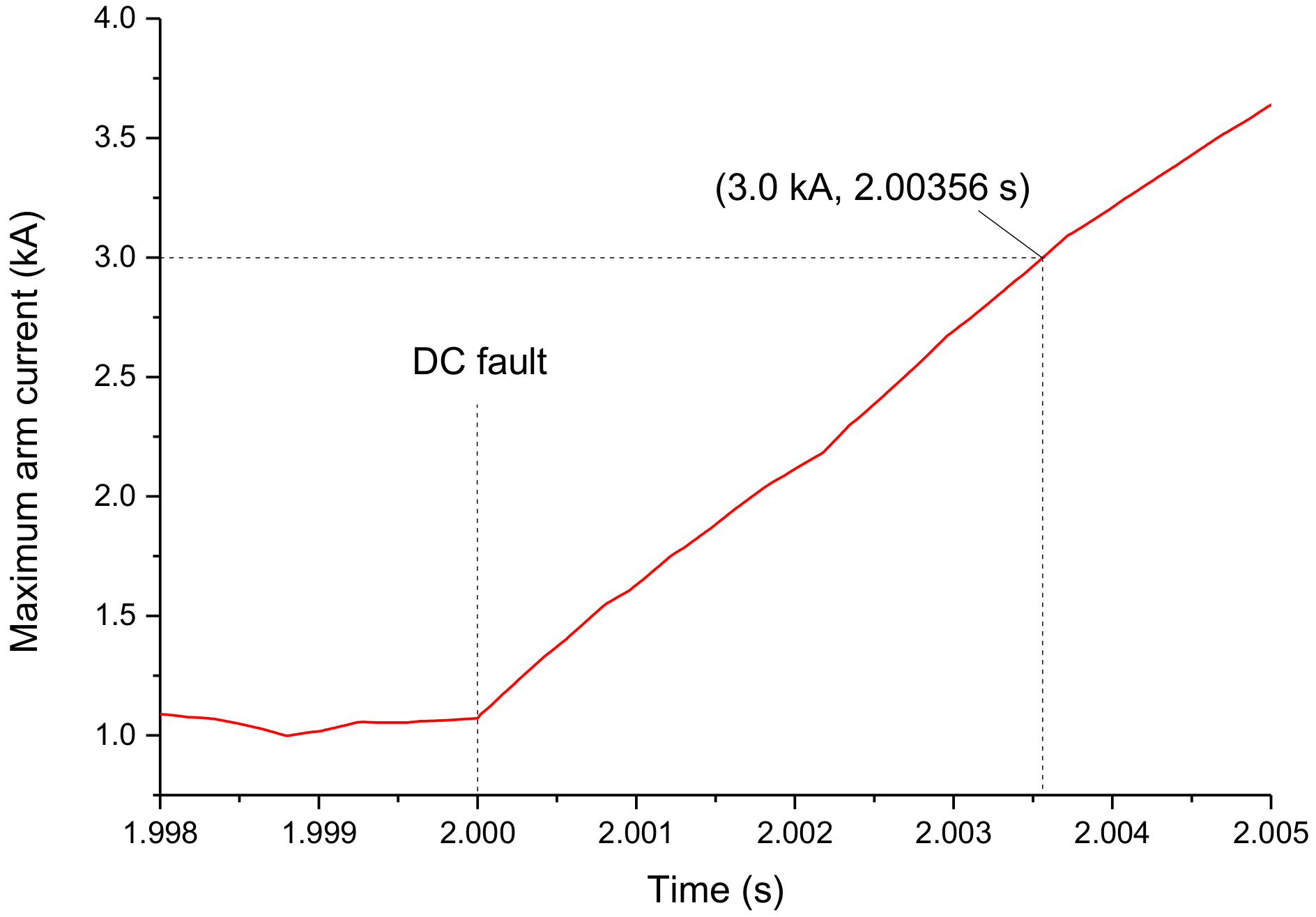
Figure 12.
DC current of MMC after blocking.

Figure 13.
DC current of MMC with solution 1.

Figure 14.
DC current of MMC with solution 2 when AC system is considered.

Figure 15.
DC current of MMC with solution 2 when AC system is not considered.
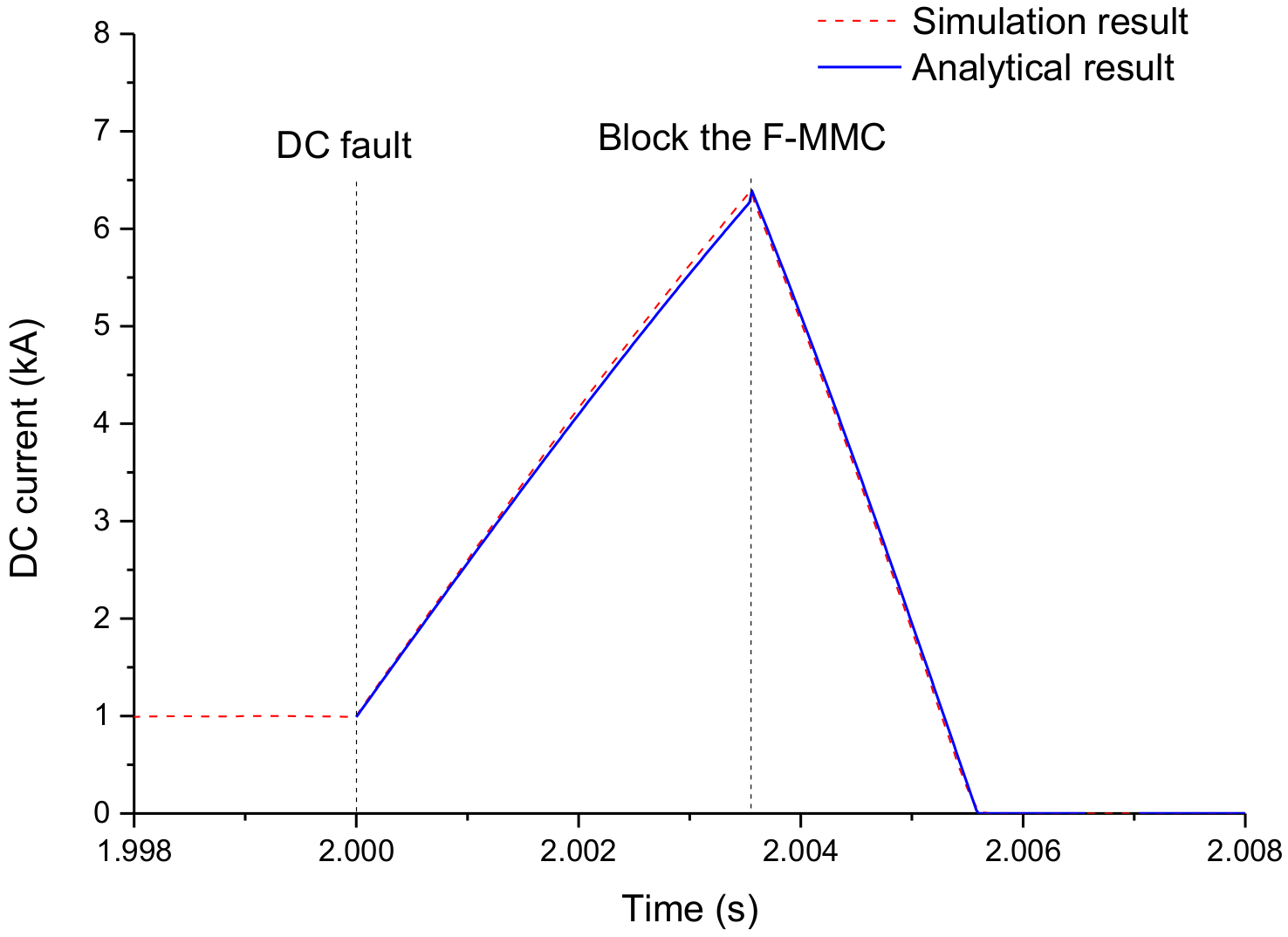
Figure 16.
DC current of MMC with solution 3.

Table 1.
Main Circuit Parameters of the MMC.
| Items | Values | |
|---|---|---|
| AC Side | Rated capacity | 400 MVA |
| Grid side AC voltage | 230 kV | |
| Transformer MVA | 450 MVA | |
| Transformer ratio | 230 kV/208 kV | |
| leakage inductance | 10% | |
| DC Side | Rated DC voltage | 400 kV |
| Smoothing reactor | 200 mH | |
| Converter | Number of SMs per arm | 20 |
| SM capacitance | 666 μF | |
| Capacitor voltage | 20 kV | |
| Arm inductance | 76 mH | |
Table 2.
Key quantities of the system with different solutions.
| Fault Clearance Time (ms) | Maximum Fault Current (kA) | Converter Blocked | |
|---|---|---|---|
| Solution 1 | 9318 | 10.8 | Yes |
| Solution 2 | 6.26 | 6.4 | Yes |
| Solution 3 | 8.06 | 6.0 | No |
© 2018 by the authors. Licensee MDPI, Basel, Switzerland. This article is an open access article distributed under the terms and conditions of the Creative Commons Attribution (CC BY) license (http://creativecommons.org/licenses/by/4.0/).
Share and Cite
MDPI and ACS Style
Xu, Z.; Xiao, H.; Xiao, L.; Zhang, Z. DC Fault Analysis and Clearance Solutions of MMC-HVDC Systems. Energies 2018, 11, 941. https://doi.org/10.3390/en11040941
AMA Style
Xu Z, Xiao H, Xiao L, Zhang Z. DC Fault Analysis and Clearance Solutions of MMC-HVDC Systems. Energies. 2018; 11(4):941. https://doi.org/10.3390/en11040941
Chicago/Turabian StyleXu, Zheng, Huangqing Xiao, Liang Xiao, and Zheren Zhang. 2018. "DC Fault Analysis and Clearance Solutions of MMC-HVDC Systems" Energies 11, no. 4: 941. https://doi.org/10.3390/en11040941
Note that from the first issue of 2016, this journal uses article numbers instead of page numbers. See further details here.