Short-Term Electricity Demand Forecasting Using a Functional State Space Model


1
Enercoop, 75019 Paris, France
2
ERIC, Université de Lyon, Lyon 2, 69676 Bron Cedex, France
*
Authors to whom correspondence should be addressed.
Energies 2018, 11(5), 1120; https://doi.org/10.3390/en11051120
Submission received: 5 February 2018
/
Revised: 20 April 2018
/
Accepted: 24 April 2018
/
Published: 2 May 2018
(This article belongs to the Special Issue Data Science and Big Data in Energy Forecasting)
Abstract
:In the past several years, the liberalization of the electricity supply, the increase in variability of electric appliances and their use, and the need to respond to the electricity demand in real time has made electricity demand forecasting a challenge. To this challenge, many solutions are being proposed. The electricity demand involves many sources such as economic activities, household need and weather sources. All of these sources make electricity demand forecasting difficult. To forecast the electricity demand, some proposed parametric methods that integrate main variables that are sources of electricity demand. Others proposed a non parametric method such as pattern recognition methods. In this paper, we propose to take only the past electricity consumption information embedded in a functional vector autoregressive state space model to forecast the future electricity demand. The model we proposed aims to be applied at some aggregation level between regional and nation-wide grids. To estimate the parameters of this model, we use likelihood maximization, spline smoothing, functional principal components analysis and Kalman filtering. Through numerical experiments on real datasets, both from supplier Enercoop and from the Transmission System Operator of the French nation-wide grid, we show the appropriateness of the approach.
1. Introduction
Important recent changes in electricity markets make the electricity demand and production forecast a current challenge for the industries. Market liberalization, increasing use of electronic appliances and the penetration of renewable electricity sources are just a few of the numerous causes that explain the current challenges [1]. On the other side, new sources of data are becoming available notably with the deployment of smart meters. However, access to these individual consumers’ data is not always possible (when available) and so aggregated data is used to anticipate the load of the system.
Load curves at some aggregate level (say regional or nation-wide) usually present a series of salient features that are the basis of any forecasting method. Common patterns are long-term trends, various cycles (with yearly, weekly and daily patterns) as well as a high dependence on external factors such as meteorological variables. We may separate these common patterns into two sets of effects. On one side, the effects linked to the social and economical organisation of the human activity. For instance, the calendar structure induces its cycle to the electrical demand: load needs during week days are higher than during weekends, and load during daylight is higher than during the night; holidays also have a large impact on the demand structure. Notice that these effects are mostly deterministic in their nature, that is they can be predicted without error. On the other side, we found the effects connected to the environment of the demand—for instance, the weather, since the demand usually depends on variables such as air temperature, humidity, wind speed and direction, dew point, etc., but also variables connected to exceptional events such as strikes or damages on the electrical grid that may affect the demand. While weather is still easier to anticipate than exceptional events, both effects share a stochastic nature that makes them more difficult to anticipate.
While only recorded at some time points (e.g., each hour, half-hour or quarter-hour), the electricity load of the system is a continuum. From this, one may consider mathematically the load curve as a function of time with some regularity properties. In fact, electrical engineers and forecaster usually represent the load curve as a function instead of a sequence of discrete measures. Then, one may study the electrical load as a sequence of functions. Recently, attention has been paid to this kind of setting, which is naturally called functional time series (FTS). A nice theoretical framework to cope with FTS is within the autoregressive Hilbertian processes, defined through families of random variables taking values on a Hilbert space [2,3]. These processes are strictly stationary and linear, which are two constrictive assumptions to model the electrical load. An alternative to linearity was proposed in [4] where the prediction of a function is obtained as a linear combination of past observed segments, using the weights induced by a notion of similarity between curves. Although the stationary assumption of the full time series is still too strong for the electrical load data [5], corrections can be made in order to render the hypothesis more reasonable. First, one may consider that the mean level of the curves presents some kind of evolution. Second, the calendar structure creates on the data at least two different regimes: workable and non workable days. Of course, the specific form of the corrections needed should depend on the nature of the model used to obtain the predictions.
State-space models (SSM) and the connection notion of Kalman filter are an interesting alternative to cope with nonlinearity and non stationary patterns of the electrical data. Let us mention some references where SSM have been used to forecast load demand. Classical vector autoregressive processes are used in [6] under the form of SSM to compare the predictive performance with respect to seasonal autoregressive processes. The main point in [7] is to combine several machine learning techniques with wavelet transforms of the electrical signal. SSM are then used to add adaptability to the proposed prediction technique. Since some of the machine learning tools may produce results that are difficult to interpret, the authors in [8] looks for a forecasting procedure based on SSM that is easier to analyse making explicit the dependence on some exogenous variables. They use a Monte Carlo based version of the Kalman Filter to increase flexibility and add analytical information.
A more detailed model is in [9], where the authors propose to describe the hourly load curve as a set of 24 individual regression models that share trends, seasons at different levels, short-term dynamics and weather effects including non linear functions for heating effects. The equations represent 24 univariate stochastically time-varying processes that should be estimated simultaneously within a multivariate linear Gaussian state space framework using the celebrated Kalman filter [10]. However, the cumbersome of the computational burden is a drawback. A second work circumvents the problem by using a dimension reduction approach which reasonably resizes the problem into a handy number of dimension which render the use of the Kalman filter practicable [11].
Some successful uses of SSM to cope with functional data (not necessarily time series) are reported in literature—for instance, by using common dynamical factor as in [12] to model electricity price and load, or as in [13] to predict yield curves of some financial assets in addition to [14] where railway supervision is performed thanks to a new online clustering approach over functional time series using SSM.
Inspired by these ideas, we push forward the model in [11] to describe now a completely functional autoregressive process whose parameter may eventually vary on time. Indeed, at each time point (days in our practical case), the whole functional structure (load curve) is described through the projection coefficients on a spline basis. Then, using a functional version of principal components analysis, the dimension of the representation is reduced. The vector of spline coefficients is then used as a multivariate autoregressive process, as in [15]. Thus, our approach is completely endogenous but with the ability of incorporating exogenous information (available at the time of the forecast) as covariates.
This paper will be structured as follows. In Section 2, we describe the model we propose for forecasting electricity demand. We present the functional data, functional data representation in splines basis, the state space model that we propose and model estimation methods. Section 3 is proposed to show a model inference on a simulated dataset. We will talk about Kalman filtering and smoothing, functional principal component analysis. Section 4 will describe the experiments we make on real data with simple application of our procedure at the aggregation level of a single supplier. We then explore, in Section 5, some corrections and extension to the simple approach in order to take into account some of the non stationary patters present in the data. Additional experiments are the object of Section 6, where we predict at the greater national aggregation level. The article concludes in Section 7 where some future lines of work are discussed.
2. Materials and Methods
We introduce in this section the notation and we construct the prediction method. For convenience, Table 1 sums up the used nomenclature including all variables, acronyms, indexes and constants defined in the manuscript, in order to make the text more clear and readable.
The starting point of our modeling is a univariate continuous-time stochastic process . To study this process, a useful device [2] is to consider a second stochastic process , which is now a discrete-time process and at each time step it takes values on some functional space. The process X is derived from Z as follows. For a trajectory of Z observed over the interval , we consider the n subintervals of form such that . Then, we can write
With this, anticipate the behavior of Z on say is equivalent to predict the next function of X. The construction is usually called a functional time series (FTS). The setting is particularly fruitful when Z presents a seasonal component of size . In our practical application, Z will represent the underlying electrical demand, will be the size of a day and so X is the sequence of daily electrical loads. Notice that X represents a continuum that is not necessarily completely observed. As mentioned in the Introduction, the records of load demand are only sampled at some discrete grid. We will discuss this issue below.
2.1. Prediction of Functional Time Series
The prediction task involves making assertions on the future value of the series having observed the first n elements . From the statistical point of view, one may be interested in the predictor
which minimizes the prediction error given the available observations at moment n. A useful model is the (order 1) Autoregressive Hilbertian (ARH(1)) process defined by
where is the mean function of X, is a linear operator and is a strong white noise sequence of random functions. Under mild conditions, Equation (2) defines a (strictly) stationary random process (see [2]). The predictor (1) for the ARH(1) process is which depends generally on two unknown quantities: the function and the operator . The former can be predicted by the empirical mean . The alternative for the latter is to predict by say and obtain the prediction , or to estimate directly the application of over the last observed centered function. Both variants needs an efficient way to approximate the possibly infinite size of either the operator or the function which are then estimated (see discussion below on this point).
The inherent linearity of Equation (2) makes this model not flexible enough to be used on electricity load forecast. Indeed, having only one (infinite-dimensional) parameter to describe the transition between any two consecutive days is not reasonable. Variants have been studied. We may mention [16] which incorporate weights in Equation (2) making the impact of recent functions more important; the doubly stochastic ARH model that considers the linear operator to be random [17]; or the conditional ARH where an exogenous covariate drives the behavior of [18]. In the sake of more flexibility, we aim to make predictions on a time-varying setting where the mean function and the operator are allowed to evolve.
2.2. Spline Smoothing for Functional Data
In practice, one only disposes a finite sampling observed eventually with noise, from the trajectory of the random function . Then, one wishes to approximate from the discrete measurements. A popular choice is to develop over the elements of a basis , which is to write
where the coefficients are the coordinates resulting of projecting the function x on each of the elements of the basis. Among the several bases usually used, we choose to work with a B-spline basis because they are adapted to cope with the nature of the data we want to model and have nice computational properties.
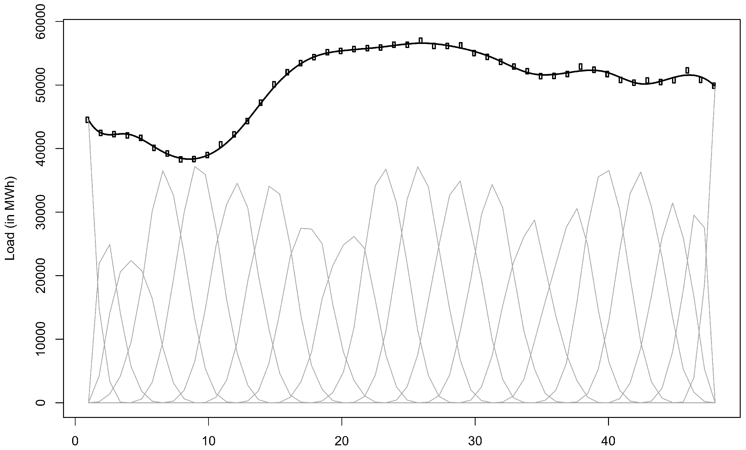
B-splines is a basis system adapted to represent splines. In our case, we use cubic spline that is 3th-order polynomial piecewise functions. The connections are made at points called knots in order to join-up smoothing, which is warranting the continuity of the second order derivative. An appealing property of B-spline is the compact support of its elements that gives good location properties as well as efficient computation. Figure 1 illustrates this fact from the reconstruction of a daily load curve. The B-spline elements have a support defined over compact subintervals of horizontal axis.
Another important property is that, at each point of the domain, the sum of the spline functions is 1. Since the shape of the spline functions on the border knots are clearly different, this fact is clearly observed on the extreme points of the horizontal axis where only one spline has a non null value. Together with the regularity constraints and the additional knots on the extreme support, these points are subject to a boundary condition. Figure 1 illustrates this important issue concerning the behavior of the boundaries. To avoid this undesirable effect, we will use a large number of spline functions on the basis that empirically allows for reducing the boundary condition.
2.3. Functional Principal Components Analysis
Like in multivariate data analysis, Functional Principal Components Analysis (FPCA) provides a mechanism to reduce the dimension of the data by a controlled lost of information. Since data in FDA are of infinite dimension, some care must be given to the sense of dimension reduction. Indeed, what we look for is a representation of the functions like the one in (3) with a relatively low number of basis functions that are now dependent on the data. Moreover, if we demand also that the basis functions form an orthonormal system, then the solution is given by the elements of the eigendecomposition of the associated covariance operator (i.e., the functional equivalent to the covariance matrix) [19].
However, the problem is that these elements are functions and so of infinite dimension. The solution is to represent themselves into a functional basis system (for instance, the one presented on the precedent section). Thus, the initial curve can be approximated in the eigenfunctions basis system:
where the number p of eigenfunctions, expected to be relatively small, will be chosen as such according to the error of approximation of the curves.
Since the representation system may be non orthogonal, then it can be shown that the inner product needed in FPCA is connected to the properties of the representational basis system.
Then, the notion of dimension reduction can be understood when one compares the lower number of eigenfunctions with respect to the number of basis functions needed to represent an observation. FPCA reduction of a representation dimension, which will yield a dramatic drop of the computational time of the model we describe next.
2.4. State Space Model
State Space Models (SSM) are a powerful useful tool to describe dynamic behavior of time evolving processes. The shape of the load curve may present long-term changes that induce non stationary patterns on the signal. Taking into account these changes is one of the challenges of electricity demand forecast.
The linear SSM [10] includes two terms. An inertial term in the form of an intrinsic state of the whole system being modeled. The observed output is a function of the state, some covariate and a noise structure. The state evolution over time is modeled as a linear equation involving the previous state and other observed variables summarized in a vector . The general formulation is given by:
where is the target variable observed at time i, is a vector of predictors, the state at time i is represented as , and are known matrices, and and are the noise and disturbance processes usually assumed to be independent Gaussian with zero-mean and its respective covariance matrices and , which usually contains unknown parameters.
The evolution of the states are useful to understand the system. Using the celebrated Kalman Filter and smoothing, one is able to extract information about the underlying state vector [10]. The one-step-ahead prediction and prediction error are respectively
In addition, their associated covariance matrices are of interest so let us define and . Since these definitions use recursion, an important step is its initialization. When the observations are unidimensional, an exact diffusion method can be used from uninformative diffuse prior. However, the method may fail with multivariate observations because the diffusion phase can yield into a non invertible matrix. Moreover, even when is invertible, computations become slow due to its dimensionality. It is however possible to obtain an univariate alternative representation of (5) that theoretically reduces computational cost of the Kalman filter and allows one to use the diffuse initialization.
2.5. A Functional State Space Model
Approaches of SSM in continuous-time also exists. For instance, Ref. [10] presents the simple mean level model. There, the random walk inherent to the state equation is replaced by a Brownian motion that drives the time-varying mean level. Early connections between FDA and SSM yielded derivations of a SSM with the help of FDA. For example, Ref. [22] uses spline interpolation to approximate the behavior of a time dependent system that is described by a space model.
Our choice is to keep the time discrete by allowing the observations to be functions or curves. A similar idea is behind the model in [14] where functions are used to represent observation on a SSM model, but only dependence between states is considered.
Let us consider the vector as the p FPCA scores resulting from the projection of , the load curve for day i, into the eigenfunctions basis system. Then, we may represent an autoregression system by replacing the covariate by the past load curve, or more precisely by its spline coefficients .
We propose the following Functional State Space Model (FSSM):
As before, the disturbance terms and follow independent Gaussian distribution with zero mean vector and generally unknown variance matrices and . The sizes of these matrices are in a function of p, the number of FPCA scores retained on the approximation step discussed above.
In order to keep the computation time under control while keeping some flexibility on the modeling, we focus on three structural forms of matrices and : full, diagonal and null, which yields six possible models. Table 2 summarizes the variants as well as the number of parameters to be estimated on the covariance matrices. The complexity of the variant grows while going from 1 to 6. When is null, then the state equation establishes that states are simply constant on time. Diagonal structures on and assumes that all the correlations are null and so only variance terms are to be treated. Conversely, full structures allows for a maximum of flexibility letting all the covariances be free. However, the important drawback of dimensionality becomes crucial since the number of terms to be estimated if of order .
The FSSM we propose is an SSM on the FPCA scores. Another choice could have been to apply the SSM directly on the spline basis coefficients , but such choice would be computationally too expensive. It is illustrative to link these dimensions to the problem of electricity demand forecasting. Recall that the number of daily records on our load curves is 48 (sampled at half-hourly), which is prohibited to be treated within our framework. Even if this number can be easily divided by two using spline approximation, the number of coefficients would be still too high. Moreover, since the spline coefficients can not be considered independent, one would need to use full diagonal structures on the covariance matrices and eventually on . Lastly, the choice we make to reduce the dimension by using FPCA approach is then justified since, with a handy number of eigenfunctions, say less than 10, most of the variants discussed above can be easily computed.
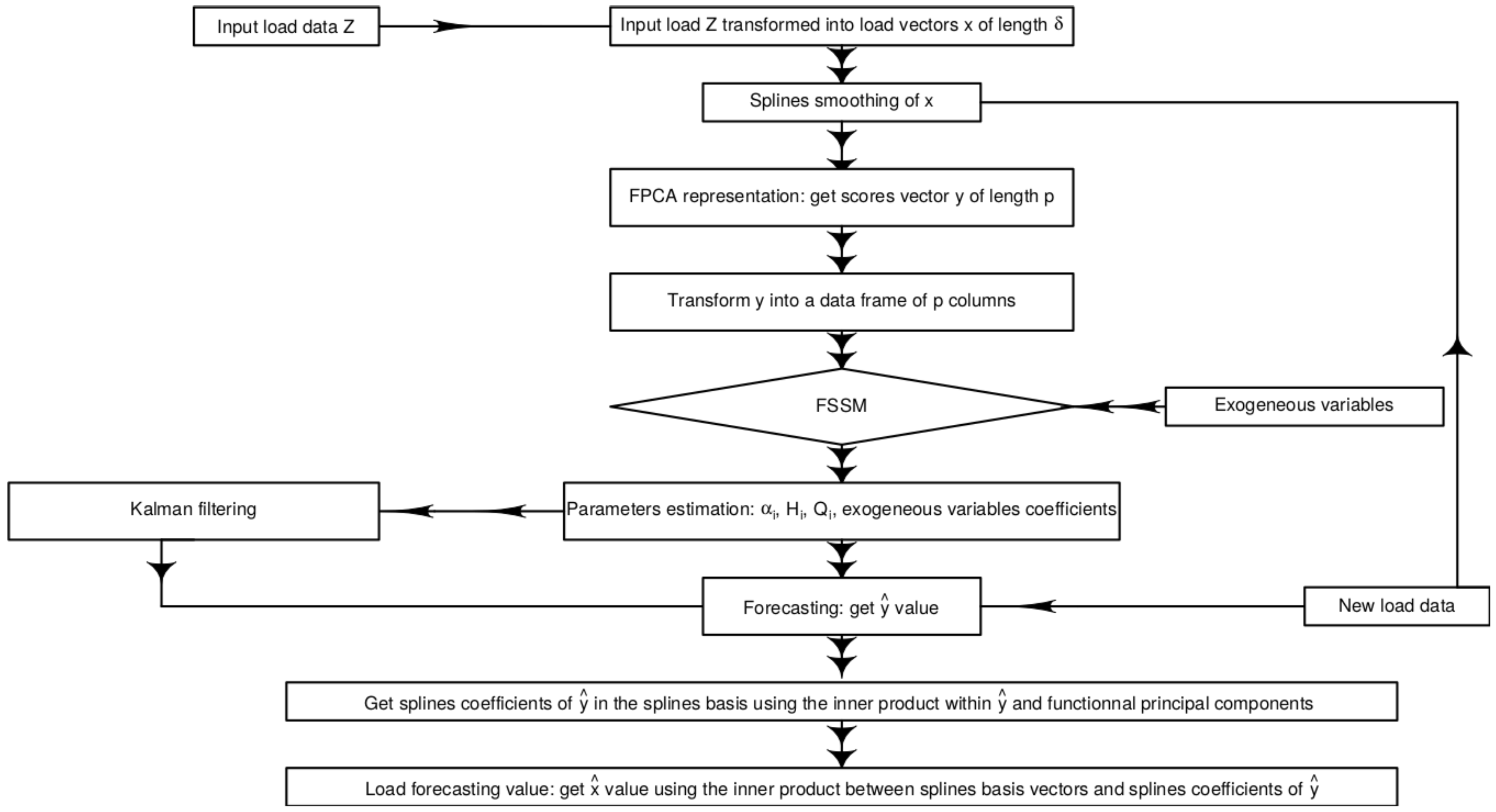
The whole prediction procedure is schematically represented as a flowchart in Figure 2.
3. Experiments on Simulated Data
We illustrate in this section our approach to forecast using the proposed functional state space models on a functional time series. There are three steps in our approach. First, we approximate the initial data using a B-spline basis. Then, an FPCA is performed using the B-splines approximations of the curves. Finally, a fit of the FSSM is obtained. Prediction can then be done by applying the recursion equations on the last estimated state. The resulting predicted coefficients are then put into the functional expansion equations (see Equations (3) and (4)) to obtain the predicted function. For the experiments, we use the statistical software R [23] to fit our model with the packages fda [24] for spline approximation and FPCA computation and KFAS [20] for the FSSM estimation.
3.1. Simulation Scheme
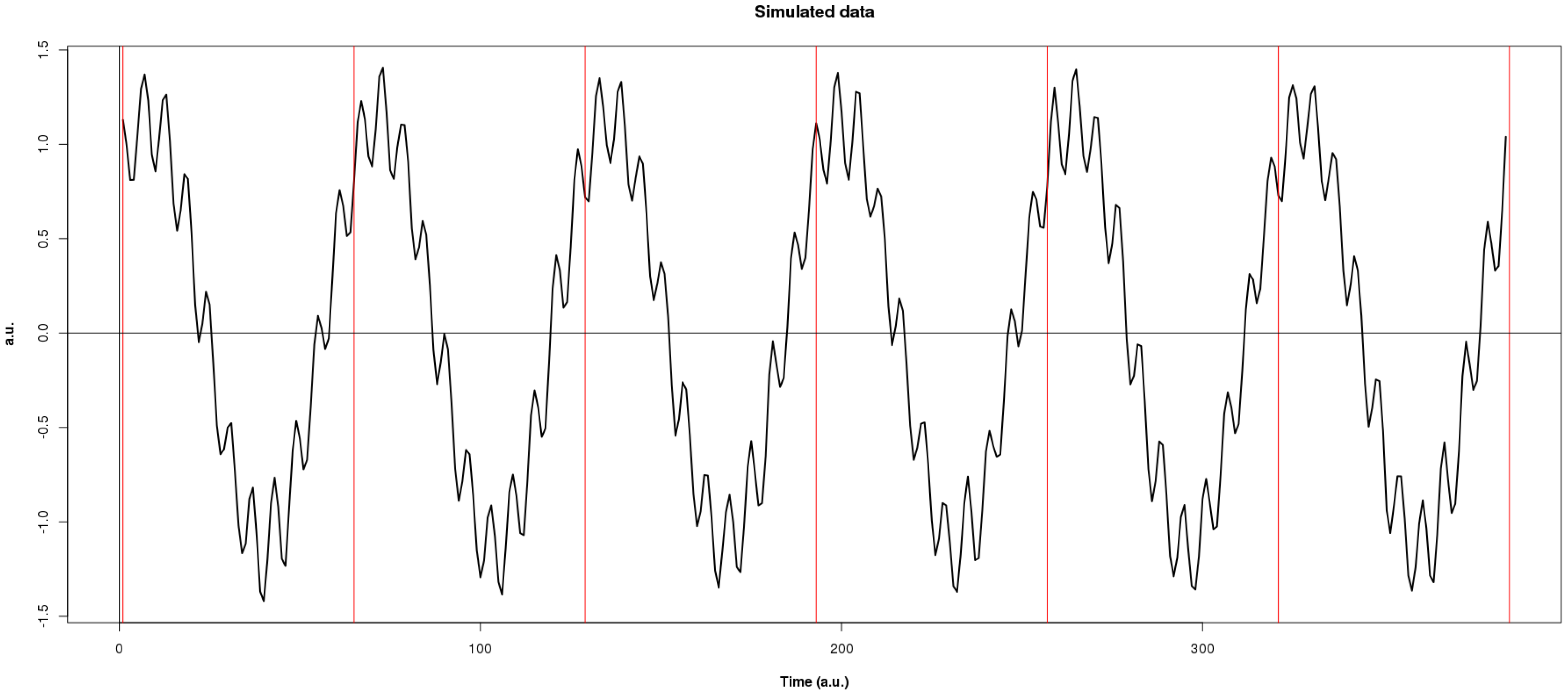
Let us consider a process Y generated as follows:
where is strong white noise process (i.e., an independent and identical distributed zero-mean normal random variables ). Following [4], we set , and , and . Expression (7) is evaluated on discrete times ranging from 1 to , where n is the number of functions of length . Then, we consider the segments of length as a discrete sampling of some unobserved functional process.
3.2. Actual Prediction Procedure
For each model variant, we build and fit the FSSM with the first 26 segments on the simulated signal. That is, each segment is projected on the B-spline basis, and these projections are used in an FPCA. We let the number p of principal components as a tune parameter of the whole procedure. Parameters are estimated and the states are filtered and smoothed as described in Section 2. The last state, together with the last segment coefficients are then used to predict the coefficients of the next segment of the signal, which is naturally not used in the estimation of the model. Using the reconstruction expression, the actual predicted segment is obtained that closes a prediction cycle.
In order to provide more robust prediction measures, several prediction cycles are used where a sequential increment of the train dataset is done. In what follows, we report results on four prediction cycles following the one-segment-ahead rolling basis described.
3.3. How We Measure Prediction Quality
There are three steps through which the prediction quality must be measured: the splines representation quality of the initial functions , the functional principal components representation of , and the forecasting. For all these three steps of quality measurement, we use the RMSE (Root Mean-Square-Error) and the MAPE (Mean Absolute Percentage Error). For one-step-ahead forecasting of vector on time i, if we consider the length of as h ( in this case), these metrics are defined as:
The RMSE is measured in the scale of the data (e.g., kWh for our electricity demand data), and MAPE is expressed in percentage. Notice that MAPE can not be calculated if target variable is zero at some time point. While this is quite unlikely in practice, our simulated signal may present values quite close to zero making MAPE to be unstable. However, this measure is useful to compare prediction performance between signals of different mean magnitude.
3.4. Results
3.4.1. Spline Representation and Reconstruction
To represent the simulated data, we use cubic splines using a regular grid for the knots (with augmented knots on the extremes). To avoid cutting down predictive power of our forecast model, we may want to retain here as many spline coefficients as possible (in our case 63). However, we have to make a special point here since a boundary condition may yield artefacts on the spline coefficients near the boundaries. A simple way to reduce this problem was to choose this number of splines (and so the length of the interior knots) to be about 59. This choice produces reasonable quality reconstructions with a MAPE error less than 0.18%.
3.4.2. Functional Principal Components
The reconstruction quality of the initial functions highly depends on the number of principal components. Of course, the quality of the forecasts will also be impacted by this choice.
Table 3 reports the reconstruction quality as mean MAPE and RMSE for two, three and four principal components.
3.4.3. Forecasting Results
In this topic, we discuss the forecasting errors for each choice of the structure of the matrices and . We take cases of null, diagonal and full matrices and , as described in Table 2. Table 4 reports RMSE and MAPE values for the forecasting of the simulation data. Both mean and standard deviation are presented. Better prediction performances produce lower MAPE and RMSE. On the one hand, as expected, the number of principal components retained has a large impact on the mean prediction performance. When only two principal components are kept, the prediction error is unreasonably large due to a poor reconstruction. On the other hand, there is no clear advantage for any variant since the standard deviations are large enough to compensate any pairwise difference. This is mainly due to the very small number of prediction segments. Variants with null matrix are slightly more performant (e.g., smaller errors). This would indicate that a static structure is detected where no time-evolving parameters are needed to predict the signal, which is the true nature of the simulated signal.
Finally, we compare now the variants from the computational time needed to obtain the prediction. We can see in Table 5 that differences in computing times are significant since standard deviations are quite small. For a fixed number of principal components, there is a clear ranking that can be obtained where the more parsimonious structures produce smaller computing times. Conversely, when the number of principal components increases the computation time increases. However, the increment is more important for the variants of covariances matrices having more parameters.
4. Experiments on Real Electrical Demand Data
We centre the experiments on this section around the French supplier Enercoop (enercoop.fr), one of the new agents appearing with the recent liberalization of the French electrical market. Electricity supplied by Enercoop is from green renewable electricity plants owned by local producers everywhere in France. The utility has several kind of customers such as householders, industries as well as small and medium-sized enterprise (SME) with different profiles of electricity consumption. People with households, for example, use electricity mainly for lightning, heating and, sometimes cooling and cooking. The main challenge for Enercoop is electricity demand and production and so anticipation of load needs is crucial for the company. We work with the aggregated electricity data that is the simple sum of all the individual demands.
We first introduce the data paying special attention to those salient features that are important for the prediction task. Then, we introduce a simple benchmark prediction technique based on persistence that we compare to the naive utilization of our prediction procedure. Next, in Section 5, we study some simple variants constructed to cope with the existence of non stationary patterns.
4.1. Description of the Dataset
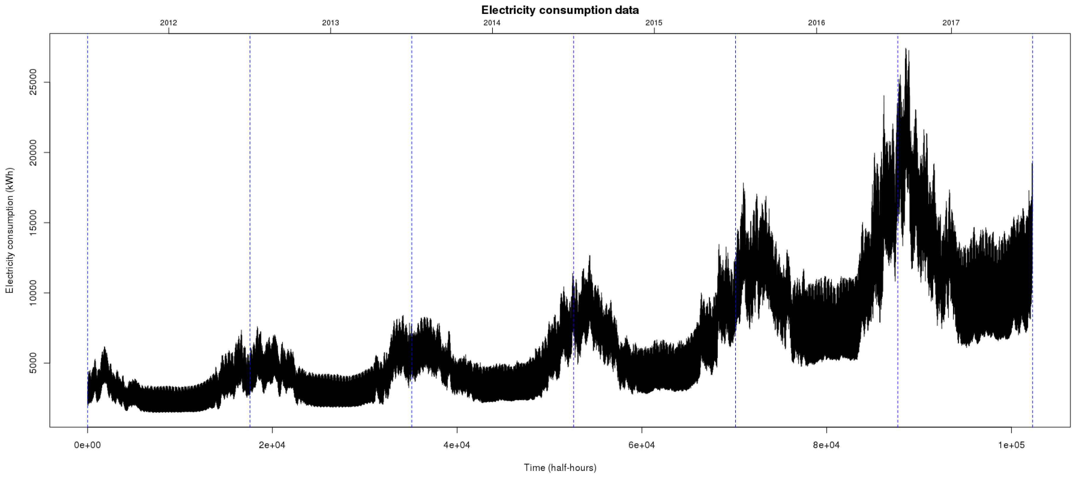
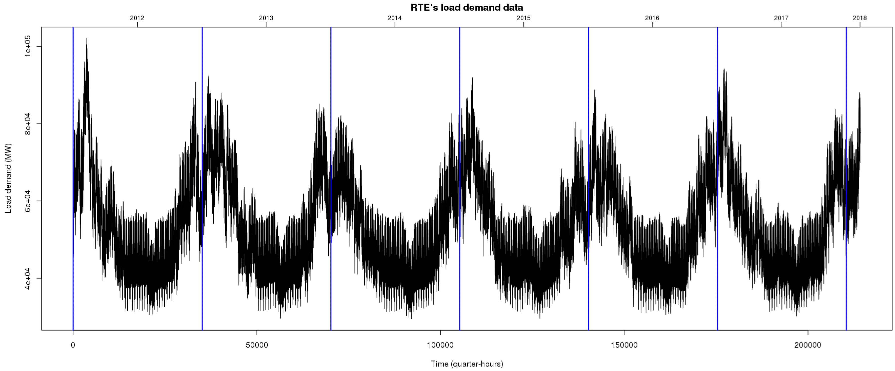
Let us use some graphical summaries to comment on the features of these data. Naturally, we adopt the perspective of time series analysis to describe the demand series. Figure 4 represents the dataset that consists of half-hourly sampled records over six years going from 1 January 2012 to 31 December 2017. Vertical bars delimits years that are shown on top of the plot. Each record represents the load demand measured in kWh.
First, we observe a clear, growing long-term trend that is connected to a higher variability of the signal at the end of the period. Second, an annual cycle is present with lower demand levels during the summer and higher during winter. Both the industrial production calendar and the weather impacts the demand, which explains this cyclical pattern.
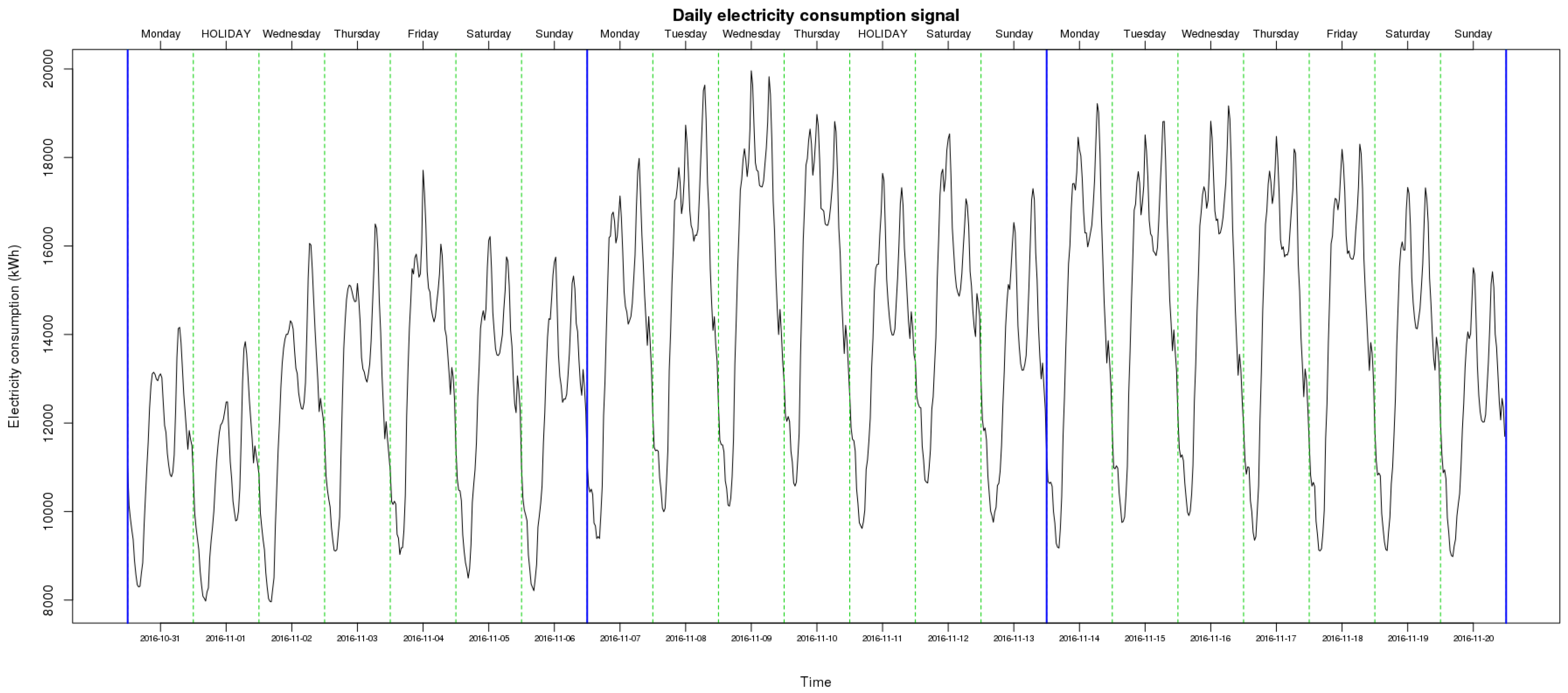
Figure 5 shows the profile of daily electricity consumption for a period of three weeks (from 31 October 2016 to 20 November 2016). This unveils new cycles presented in data that can be seen as two new patterns: the weekly one and the daily one. The former is the consequence of how human activity is structured around the calendar. Demand during workable days is larger than during weekend days. The latter is also mainly guided by human activity with lower demand levels during the nighttime, and the usual plateau during the afternoon and peaks during the evening. However, a certain similarity can be detected among days. Indeed, even if the profile of Fridays is slightly different, the ensemble of workable days share a similar load shape. Similarly, the ensemble of weekends form a homogeneous group. Holiday banks and extra days off may also impact the demand shape. For instance, in Figure 5, the second segment, which corresponds to 1st November, is the electrical demand on a bank holiday. Even if this occurs on a Tuesday, the shape of load of these days and the preceding one (usually an extra day off) are closer to weekend days.
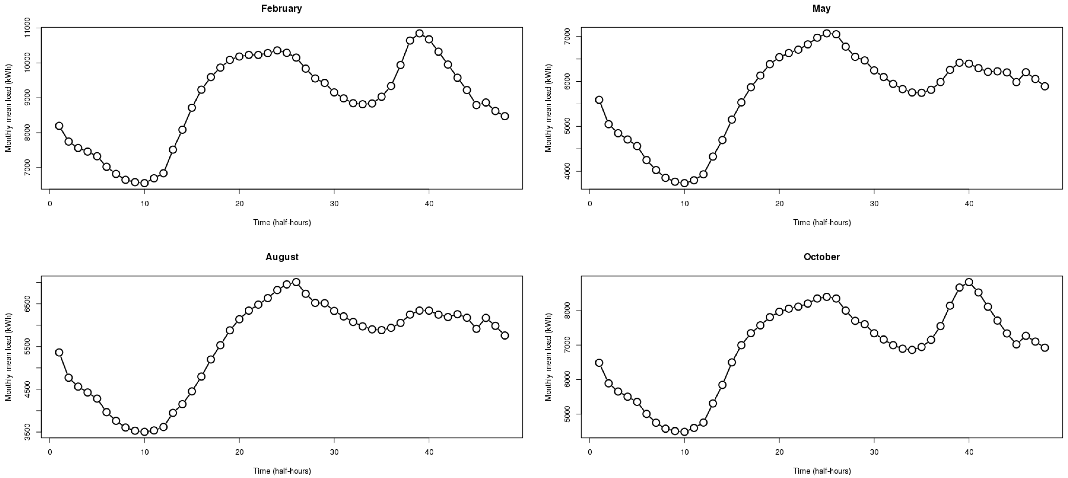
We may also inspect the shape of the load curve across the annual cycle. A simple way to do this is to inspect the mean form between months. Figure 6 describes four monthly load profiles, where each month belongs to a different season of the year. Some differences are easy to notice—for instance, the peak demand is during the afternoon in Autumn and Winter but at midday in Spring and Summer. Others are more subtle, like the effect of daylight savings time clock change, which horizontally shifts the whole demand. Transitions between the cold and warm seasons are particularly sensitive for the forecasting task, especially when the change is abrupt.
4.2. Spline and FPCA Representation
As before, we report on the reconstruction error resulting from the spline and FPCA representations.
For comparison purposes, we compute the error criteria for five choices on the number of splines (12, 24, 40, 45 and 47 splines) on the reconstruction of the coded functions. Table 6 shows the MAPE and RMSE between the reconstruction and the real load data. As expected, the lower the number of splines, the higher the reconstruction error. This shows that, using only spline interpolation, our approach is not pertinent because a relatively large number of spline coefficients is needed. The extremest case of 12 splines, which would make the computing times reasonable, produces a too large MAPE of 1.310%, which hampers the performance of any forecasting method based on this reconstruction. On the other extreme, using 47 cubic splines to represent the 48-length discrete signal of the daily demand produces boundary effects that will dominate the variability of the curves.
Since spline approximation is connected to the FPCA in our approach, we may check the reconstruction quality for all the choices issued from the crossing of the selected number of splines and a number of principal component between 2 and 10. Table 7 shows the MAPE and RMSE of the reconstructions obtained by each of the possible crossings. We may target a maximum accepted MAPE value of 1% in reconstruction. Then, there are just a few options, most of them with very close MAPE values. In what follows, we choose to work with 45 cubic splines and 10 principal components.
4.3. Forecasting Results
Forecasting is done in a rolling basis over one year in the data. Load data from 1 January 2012 to 30 October 2016 is used as a training dataset and, as a testing dataset, we choose a period from 31 October 2016 to 30 October 2017. Predictions are obtained at horizons one-segment ahead. This means that, actually, we are making predictions for the next 48 time steps (1 day) if we adopt a traditional time series point of view. Once the prediction is obtained, we compare it with the actual data and incorporate the observation into the training dataset. Thanks to the recursion in the SSM, only an update step is necessary here.
To give a comparison point to our methodology, we propose using a simple but powerful benchmark based on persistence forecasting.
4.3.1. Persistence-Based Forecasting
A persistence-based forecasting method for a functional time series equals to anticipate with the simple predictor . Thus, the predictor can be connected to the ARH model (Equation (2)) where the linear operator is the identity operator . However, this approach is not convenient since there are two groups of load profiles in the electricity demand given by workable days and the other days (e.g., weekends or holidays). We use then a smarter version of the persistence model, which takes into account the existence of these two groups. The predictor is then written
Table 8 summarizes the MAPE on prediction by type of day for the persistence-based forecasting method. We can observe that the global MAPE errors are several times the reconstruction error we observed above. There is a clear distinction between those days predicted by the previous day and the other ones (i.e., Saturdays, Sundays and Mondays). The lack of recent information for the latter group is a severe drawback and impacts its prediction performance. The increased difficulty of predicting bank holidays is translated into the highest error levels.
4.3.2. FSSM Forecasting
We now present the results for the proposed FSSM. Only the variant 1 in Table 2 is used, namely we consider the covariance matrix of the observations as diagonal and the covariance matrix of the states as null. The reason is twofold. First, we show on simulations that basic models give as satisfactory results as the more involved ones. Second, computing time must be kept into reasonable standards for the practical application.
Table 9 and Table 10 show the MAPE on prediction for days and months respectively for the FSSM approach. In comparison with the persistence-based forecasting, the global error is sensibly reduced with improvement on almost all day types. In addition, improvements are observed in all the months of the year but August (results for persistence-based forecasting are not shown). If we look at the distribution of MAPE, we see that the range is compressed with a lower maximum error but also a higher minimum error. This last effect is the price to pay for having an approximate representation of the function. We may think the MAPE on approximation as a lower bound for the MAPE on forecasting. The higher this bound, the more limited the approach is. Despite this negative result, the gain on the largest errors observed before more than compensates for the increment on the minimum MAPE and yields a globally better alternative. Among workable days, Mondays presents the higher MAPE. FSSM being an autoregressive approach, it builds on the previous days that present a different demand structure. Moreover, the mean load level of these two consecutive days is sharply different. Undoubtedly, incorporating the calendar information would help the model to better anticipate this kind of transition. Both mean load level corrections and calendar structure are modification or extensions that can be naturally incorporated in our FSSM. We discuss some clues for doing this in the next section.
5. Corrections to Cope with Non Stationary Patterns
We explore two kinds of extensions to add exogenous effects. In the first one, the days are grouped into two groups, workable and non workable days, and the prediction is done separately in each group. In the second one, the day and the month are introduced as an exogenous fixed effect in the model.
5.1. Adding Effects as Grouping Variables
We aim to tackle some of the difficulties that non stationary patterns impose on the forecasting of load data by explicitly considering two groups of days: workable (i.e., Monday, Tuesday, Wednesday, Thursday, Friday), and non workable (i.e., Saturday, Sunday and Holidays). We adapt our model FSSM described in Equation (6) by adapting it on each group separately, that is, we consider the model
The only difference between models (6) and (9) is the data used in estimation of parameters. In the case of (9), we have two groups of data, workable days and, non workable days. The structure of the matrices are the same as in the model 6, but now they are specific to each group of days. In terms of forecasting procedure, if we want to predict a workable day, we choose the data for the group workable. Similarly for non workable days, in Table 11 and Table 12, we present MAPE obtained with this procedure reported by day type and month. The results for this approach globally improve the forecast with respect to the initial model since the global MAPE decreases. In addition, reduced MAPE are obtained for most of the day types. However, we can see also that, for Saturday and Monday, the errors are significantly increased. These days are those where the transition between the groups occur. They share then the additional difficulty of not having the most recent information (that one from the precedent day) in the model. Some cold months’ predictions are not improved. Improvements are observed during summer months or months around summer. The high level load demand and variability of winter months impacts the rise of prices and thus makes these months of particular interest. The accuracy in forecasting for these months is important because bad prediction can have a large economical impact for electricity suppliers.
One thing we can also do to improve forecasting of load demand is to integrate some exogenous variables such as day types and weather variables. Day types are fixed variables and weather variables are random variables. In this paragraph, we have just implicitly introduced day types in our modeling but not as exogenous variable. In the next paragraph, we introduce in our model the variable day types.
5.2. Adding Effects as Covariates
In this paragraph, we introduce in model (6) the variables day type and months. We must have an appropriate presentation of this exogenous deterministic variables before predicting. We choose to create for each day of the week, a binary dummy variable. In total, we have eight days (including holidays) type which we use as eight dummies variables. Each variable takes values in . The value 1 corresponds to the case where the response vector is observed on the same day as the day that is being used. For example, if the response variable is observed on Sunday, the dummy variable for Sunday takes value 1. The dummy variable for Sunday will take 0 if the response vector is not observed on Sunday, but takes 1 for other day dummy variable on which it was observed. In addition, we choose a numeric variable that represents the months of the year. We would like to control the seasonal effect of the series with this variable. The months variable has 12 values representing the month of the year. Let us choose as days’ dummy variables and as the numeric months’ variable. The model (6) becomes:
, , and . and are fixed in the time but and are not fixed in time because the profile of the series changes with time. These regression coefficients can be interpreted as estimation of each day and month mean profiles of the series. Let us note . In terms of mixed linear models modeling, controls the fixed effects of the load data. Parameters estimation of (10) is a bit different when using the package KFAS that allows for estimating states’ space models parameters. In the case of the model (6), we choose a random approach to estimate , which consequently explains the random parts of the load curves. This means that we assume that exists.
Table 13 and Table 14 sum up the prediction performance of model 10 using daily and monthly MAPE respectively.
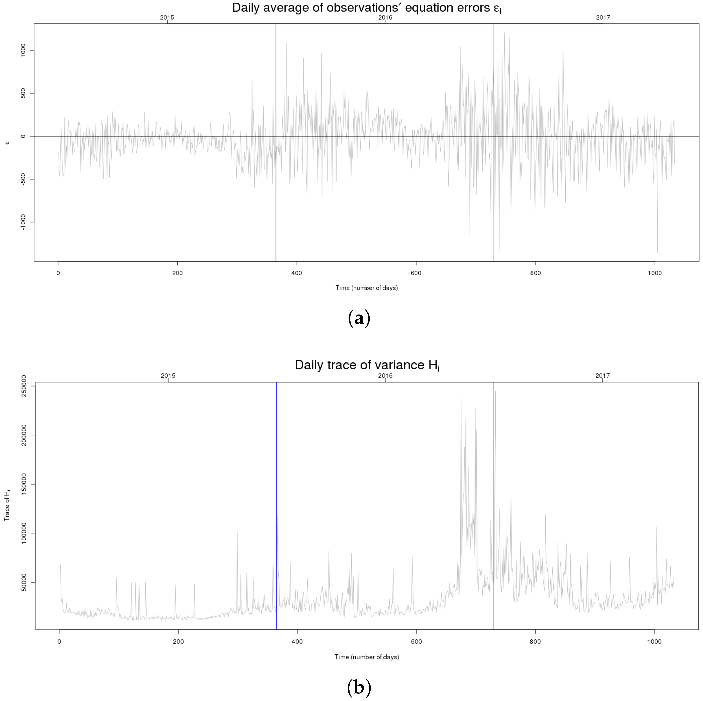
It can be observed that the global MAPE decreases. On Monday, the MAPE decreases significantly. It is still difficult to have accurate prediction in winter and spring months, except December and February. For the month of November, the great value of MAPE is due to unprecedented increase of the number of customers on November 2016. Figure 7 shows the errors of observations equation and their variance . It can be observed at the end of year 2016 (from November 2016) that there was a big change in the errors’ variance. This change comes from the change in the rhythm of electricity consumers’ subscription as clients of Enercoop. In the end of 2016, there was the COP21 (21st Sustainable Innovation Forum) in France. As Enercoop’s strategy is to support renewable electricity production and consumption; at this moment, the communication of the image of Enercoop increased in the population. Enercoop was more well known to the French public than ever. This communication brought many customers to subscribe to electricity supplied by Enercoop. For this moment, it is difficult for the model to be accurate because, at this moment, outliers’ values were being observed.
6. A Short Case Study: Prediction at a National Grid Level
We now provide a detailed case study on the construction of a forecasting model using our approach for a more aggregated signal. We move from the supplier point of view to the Transmission System Operator (TSO) point of view. Data in this section come from RTE (Réseau de Transport d’Électricité) (http://www.rte-france.com/)), the TSO of the French electrical grid. These data are openly available (http://www.rte-france.com/fr/eco2mix/eco2mix-telechargement). The size of the system is a considerably large RTE operating on the largest grid in Europe with over 100,000 km of electrical lines and routing a total gross annual consumption of over 475 TWh. For the reasons detailed below, we incorporate meteorological data in the prediction model. For this, data is obtained upon Météo-France, the national weather service in France (https://donneespubliques.meteofrance.fr/).
6.1. Salient Features on the Data
Data is retrieved from RTE API (http://www.rte-france.com/fr/eco2mix/eco2mix-telechargement) where past effective demands but also forecast load demand obtained by RTE are available. The daily load demand is recorded with 96 points per day, which is equivalent to intervals of fifteen (15) minutes.
We use a series of plots to highlight relevant features on the data that should be considered in the construction of a prediction model. The first view of the data is in Figure 8, which shows the time plot of the electrical load from 2012 until the first two months of 2018 (vertical lines separates years). When compared to Figure 5, the most important fact is the absence of a growing trend. Indeed, the gross yearly energy demand in France is quite stable during the period of study, which explains the constant trend. The annual cycle is clearly made evident with yearly larger levels of load demand during winter and lower ones during summer.
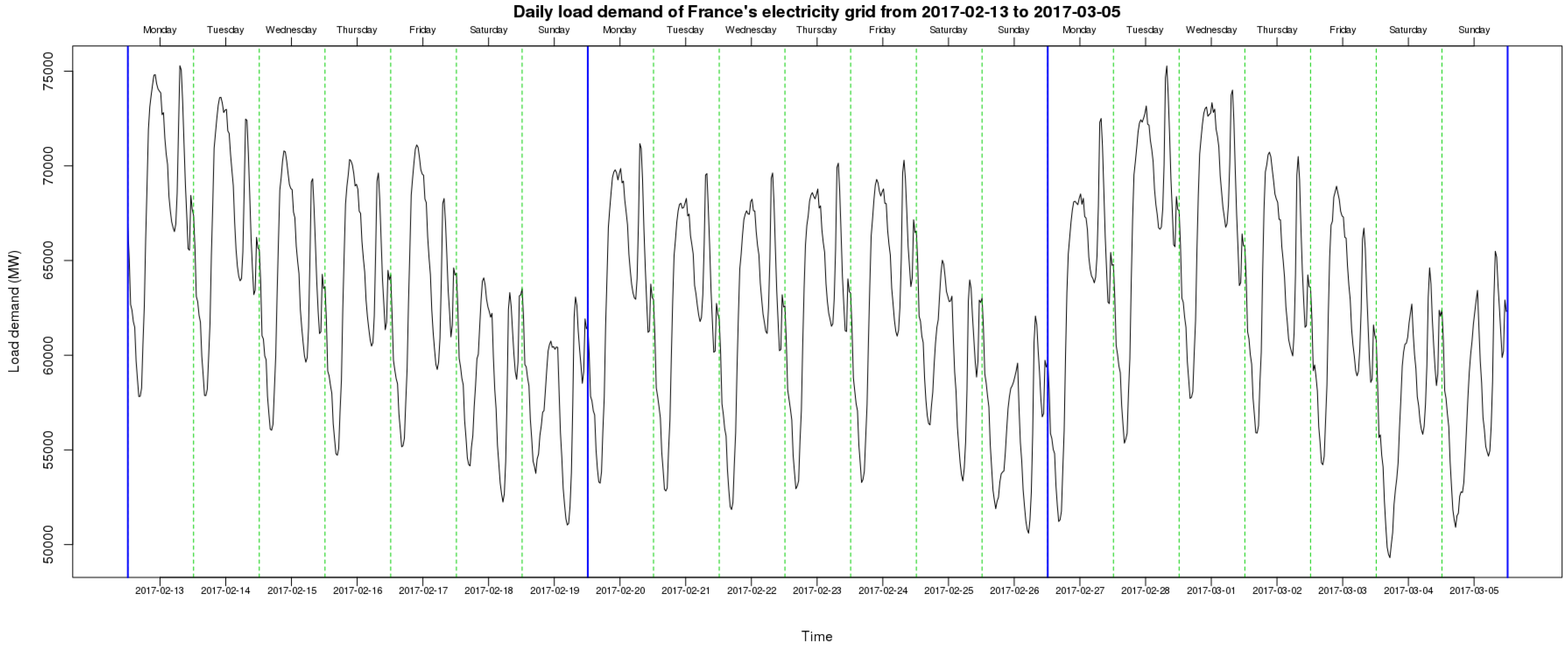
Figure 9 illustrates the daily load demand for France from 13 February 2017 to 5 March 2017. As it can be noticed, the load demand is correlated with human activities, which means that the load profile is high on workable days and low on weekends and holidays.
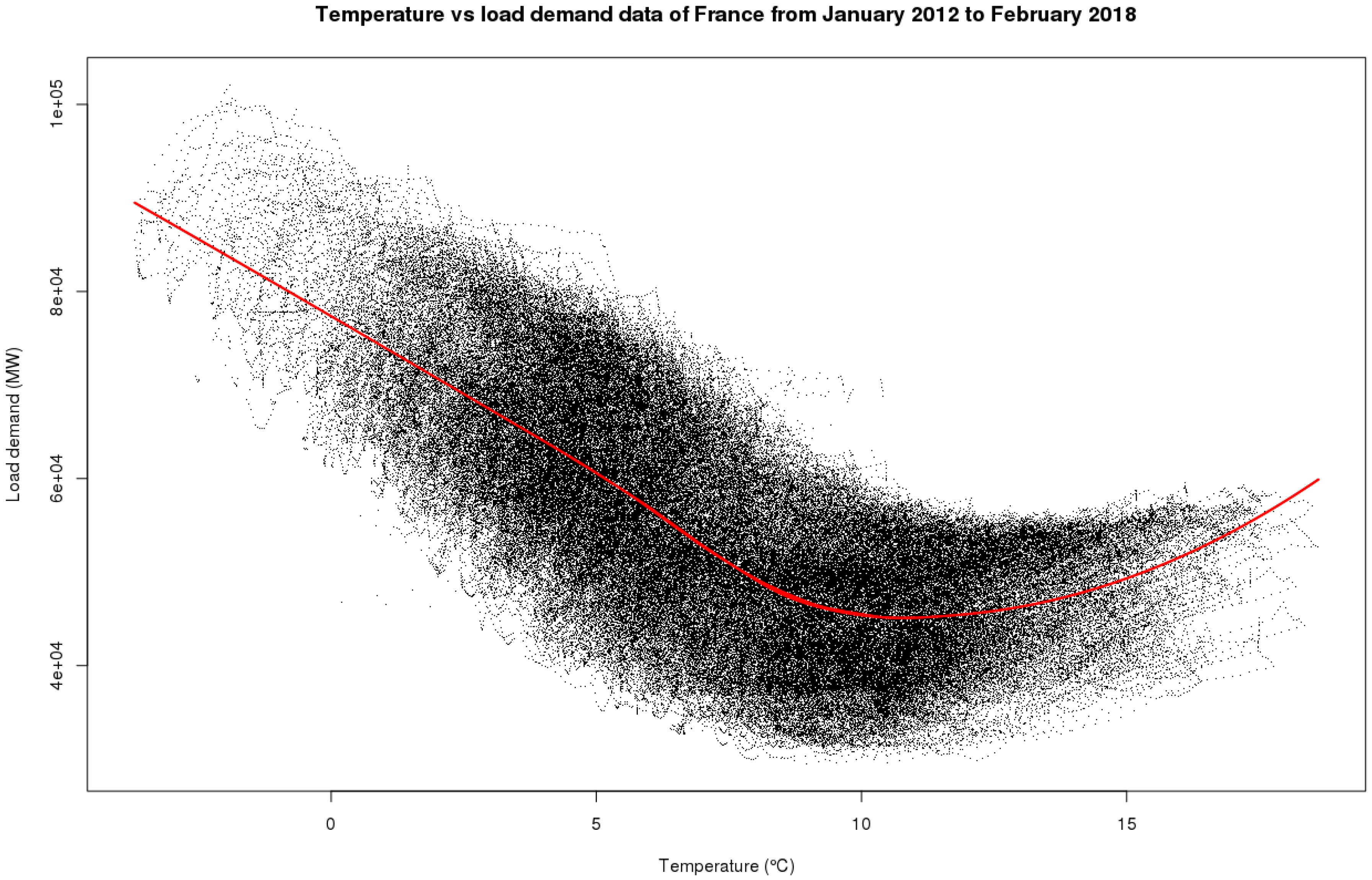
Lastly, Figure 10 represents the relationship between load demand and temperature by both a scatter plot and a smooth curve estimated non parametrically. It can be seen that demand increases with cold or hot temperatures.
6.2. Model Construction
For the FSSM training and test purposes, we use data from 1 January 2012 to 9 February 2017 as training dataset and from 10 February 2017 to 9 February 2018 for the test dataset.
For the comparison purposes, we make some experiments with model 6 and we introduced some exogenous variables. For our model training purposes, we represent the initial load demand data in a cubic splines basis (with 82 splines) and in a functional principal components basis (with 10 functions). Observing the initial load data, we can notice the annual (see Figure 8) and the week (see Figure 9) patterns in the load data. Therefore, we introduce four fixed variables , , and . In a week, we have seven days that we transform to a numeric variable NumDay, and to extract the week pattern in the load demand, we choose , . For the annual pattern, we introduce variable PosDayYear, which means position of the day in a year (position goes from 1 to 365) and . Finally, we make variables and . Year also controls the effects of months, which is why we do not need to introduce months in this model. The load demand depends on the type of the days, as it has been noticed. For this reason, we introduce the day type dummies variables as in the case of Enercoop’s load demand data forecasting. It should be noted that we add new fixed variables for RTE’s load demand data forecasting, which are different from fixed variables used for Enercoop’s load demand forecasting. The reason for this choice is the annual and weekly seasonality observed in the load demand data.
We have also observed that the load demand is a quadratic function of temperature (see Figure 10). The target temperature that we consider here is an aggregation of France’s 96 departments’ temperatures. Usually, RTE considers a few special zones, which represent all of France in terms of temperature. We do not consider this representation method in this paper. It can be observed in Figure 10 that load demand decreases with temperature below 10 °C, and increases with temperature above 10 °C. The temperatures below 10 °C describe the heating season for the load demand and the temperatures above 10 °C illustrate the cooling season for the load demand. For this reason, we define two variables and to be introduced into the model. We then define a variable as . Then, the FSSM model used for the RTE load demand data is
where , , , , and .
6.3. Prediction Performances
Table 15 and Table 16 illustrate the results of the RTE prediction model on the test period. It can be observed that forecasting MAPE is quite high during weekends and higher on holidays. The global MAPE is about 1.47%, which means in terms of RMSE to 912.12 MW.
Table 17 and Table 18 illustrate the results of our model (11). We can see that, during Saturdays and Holidays, model (11) performs better than RTE’s model. MAPE of months shows that, during February, March, May, June and October, our model performs better than the model of RTE. Nevertheless, the global MAPE for (11) is , which means 972.25 MW in terms of RMSE, which is slightly larger than for the RTE model. One way to improve our model is to introduce all variables that can change the load signal such as hydro power production with water pumping, wind power production and photo-voltaic power production and consumption.
7. Discussion and Conclusions
In a concurrent environment, electrical companies need to anticipate load demand from data that presents non stationary patterns induced by the arrival and departure of customers. Forecasting in this context is a challenge since one desires using as much past data as possible but needs to reduce the usable date to the records that describe the current situation. In this trade-off, adaptive methods have their role to play.
Figure 7 witnesses the ability that FSSM has to adapt to a certain extent to the changing environment. The impact of an external event to the electrical demand is translated into larger variability on the error and so an inflation of the trace of the errors variance matrix (cf. at the end of 2016).
Forecasting process for Enercoop’s load demand in this paper is mainly endogenous. Only some calendar information is used as an exogenous variable. However, in electricity forecasting, it is well known that weather has a great influence on the load curve. For instance, temperature impacts through the use of cooling systems in hot season and electrical heating during cold seasons. In France, this dependence is known to be asymmetrical with a higher influence of temperature on cold days. The nature of this covariable on forecasting is different to the ones we used. Indeed, while calendars can be deterministically predicted, it is not the case for the temperature. Using forecasted weather on an electrical demand forecast inserts the eventual bias and the uncertainty of the weather forecasting system to the electrical demand prediction. Integration of weather information into our model to forecast Enercoop’s load demand data, eventually changing the structure of the matrix , and obtaining prediction interval for the predictions are perspectives of future work.
For France’s grid load demand, we have integrated fixed and weather variables that enable better forecasting than in the case of Enercoop. It is possible to improve the accuracy of our model on this data if there is more time to have more information on all variables that can be introduced in the forecasting process.
In addition, only point predictions are obtained. In a probabilistic framework, one would like to have not only an idea of the mean level anticipation of the load, but also some elements about the predictive distribution of the forecast. Whether it is a whole distribution, some quantile levels or a predictive interval, this information is not trivially obtained from our approach. While SSM does provide intervals through the Gaussian assumptions coupled with the estimation of the variance matrices, FSSM has this information on the coefficients of the functional representation. Transporting this information to the whole curve needs to be studied.
Besides these technical considerations, a natural interrogation is how this model can be used in other forecasting contexts. While the work is focused on short-term prediction horizons, there is no mathematical constraint in using the model on other tight time frameworks. For instance, for a long-term horizon, one would naturally increase the sample resolution to a certainly monthly basis in which case the functional segments could represent the annual cycle. However, as it is well known in practice, predicting long-term patterns without relevant exogenous information is not the best option. Another case to consider is the presence of periodic and seasonal patterns. As it is the case, the electricity demand carries on very clear cycles (e.g., yearly, weekly, daily) that are exploited by our model in two ways. First, the smallest one is taken into consideration within the functional scheme and so all the non stationary patterns inside it are naturally taken into consideration by the model. Second, the largest ones are explicitly modelled as exogenous variables. A last case relevant to discuss is the one where the sampling of the time series is done by an irregular basis. However, in our examples, we only treated regular grid samplings, and the functional data analysis framework allows one to cope with irregular sampling in a natural way. Indeed, the data for each segment (in our case each day) is used to fit the corresponding curve (e.g., the daily load curve) and then estimate the spline coefficients. With this, the rest of the forecasting procedure remains unchanged. Of course, the proposed model could be used to forecast other kind of phenomena. The good reliability and predictability would depend on the nature of these signals.
To sum up, the presented model has enough flexibility to be used in the anticipation of energy demands in the electricity industry, providing credible predictions of energy supply, and improvement on the efficient use of energy resources. This may help to handle theoretical and practical electricity industry applications for further development of energy sources, strategic policy-making, plans of energy mix and adoption patterns [25].
References
Author Contributions
All the authors equally contributed to this work.
Conflicts of Interest
The authors declare no conflict of interest.
References
- Cugliari, J.; Poggi, J.M. Electricity Demand Forecasting. In Wiley StatsRef: Statistics Reference Online; John Wiley & Sons: Hoboken, NJ, USA, 2018. [Google Scholar]
- Bosq, D. Linear Processes in Function Spaces; Springer: New York, NY, USA, 2000. [Google Scholar]
- Álvarez Liébana, J. A review and comparative study on functional time series techniques. arXiv, 2017; arXiv:1706.06288. [Google Scholar]
- Antoniadis, A.; Paparoditis, E.; Sapatinas, T. A functional wavelet-kernel approach for time series prediction. J. R. Stat. Soc. Ser. B (Stat. Methodol.) 2006, 68, 837–857. [Google Scholar] [CrossRef]
- Antoniadis, A.; Brossat, X.; Cugliari, J.; Poggi, J.M. Prévision d’un processus à valeurs fonctionnelles en présence de non stationnarités. Application à la consommation d’électricité. J. Soc. Fr. Stat. 2012, 153, 52–78. [Google Scholar]
- Ohtsuka, Y.; Kakamu, K. Space-Time Model versus VAR Model: Forecasting Electricity demand in Japan. J. Forecast. 2011, 32, 75–85. [Google Scholar] [CrossRef]
- Nguyen, H.T.; Nabney, I.T. Short-term electricity demand and gas price forecasts using wavelet transforms and adaptive models. Energy 2010, 35, 3674–3685. [Google Scholar] [CrossRef]
- Takeda, H.; Tamura, Y.; Sato, S. Using the ensemble Kalman filter for electricity load forecasting and analysis. Energy 2016, 104, 184–198. [Google Scholar] [CrossRef]
- Dordonnat, V.; Koopman, S.; Ooms, M.; Dessertaine, A.; Collet, J. An hourly periodic state space model for modelling French national electricity load. Int. J. Forecast. 2008, 24, 566–587. [Google Scholar] [CrossRef]
- Durbin, J.; Koopman, S.J. Time Series Analysis by State Space Methods; Oxford University Press (OUP): Oxford, UK, 2012; Volume 38. [Google Scholar]
- Dordonnat, V.; Koopman, S.J.; Ooms, M. Dynamic factors in periodic time-varying regressions with an application to hourly electricity load modelling. Comput. Stat. Data Anal. 2012, 56, 3134–3152. [Google Scholar] [CrossRef]
- Liebl, D. Modeling and forecasting electricity spot prices: A functional data perspective. Ann. Appl. Stat. 2013, 7, 1562–1592. [Google Scholar] [CrossRef]
- Hays, S.; Shen, H.; Huang, J.Z. Functional dynamic factor models with application to yield curve forecasting. Ann. Appl. Stat. 2012, 6, 870–894. [Google Scholar] [CrossRef]
- Samé, A.; El-Assaad, H. A state-space approach to modeling functional time series application to rail supervision-IEEE Conference Publication. In Proceedings of the 22nd European Signal Processing Conference (EUSIPCO), Lisbon, Portugal, 1–5 September 2014. [Google Scholar]
- Holmes, E.E.; Ward, E.J.; Wills, K. MARSS: Multivariate Autoregressive State-space Models for Analyzing Time-series Data. R J. 2012, 4, 467–487. [Google Scholar]
- Besse, P.; Cardot, H. Approximation spline de la prévision d’un processus fonctionnel autorégressif d’ordre 1. Can. J. Stat. 1996, 24, 467–487. [Google Scholar] [CrossRef]
- Guillas, S. Doubly stochastic Hilbertian processes. J. Appl. Probab. 2002, 39, 566–580. [Google Scholar] [CrossRef]
- Cugliari, J. Non Parametric Forecasting of Functional-Valued Processes: Application to the Electricity Load. Ph.D. Thesis, Université Paris Sud, Paris, France, 2011. [Google Scholar]
- Ramsay, J.O.; Hooker, G.; Graves, S. Functional Data Analysis with R and MATLAB; Springer: New York, NY, USA, 2009. [Google Scholar]
- Helske, J. KFAS: Exponential Family State Space Models in R. J. Stat. Softw. Art. 2017, 78, 1–39. [Google Scholar] [CrossRef]
- Koopman, S.J.; Durbin, J. Filtering and smoothing of state vector for diffuse state-space models. J. Time Ser. Anal. 2003, 24, 85–98. [Google Scholar] [CrossRef]
- Valderrama, M.J.; Ortega-Moreno, M.; González, P.; Aguilera, A.M. Derivation of a State-Space Model by Functional Data Analysis. Comput. Stat. 2003, 18, 533–546. [Google Scholar] [CrossRef]
- R Core Team. R: A Language and Environment for Statistical Computing; R Foundation for Statistical Computing: Vienna, Austria, 2017. [Google Scholar]
- Ramsay, J.O.; Wickham, H.; Graves, S.; Hooker, G. fda: Functional Data Analysis, R Package version 2.4.7. 2017. Available online: http://CRAN.R-project.org/package=fda (accessed on 2 May 2018).
- Kyriakopoulos, G.L.; Arabatzis, G. Electrical energy storage systems in electricity generation: Energy policies, innovative technologies, and regulatory regimes. Renew. Sustain. Energy Rev. 2016, 56, 1044–1067. [Google Scholar] [CrossRef]
Figure 1.
Illustration of the representation of a daily load curve (thick line) by a rank 20 B-spline bases (thin lines).
Figure 1.
Illustration of the representation of a daily load curve (thick line) by a rank 20 B-spline bases (thin lines).

Figure 2.
Functional State Space Model (SSM) flowchart in practice.

Figure 3.
Simulated signal generated via model (7).
Figure 3.
Simulated signal generated via model (7).

Figure 4.
Electricity demand for the supplier Enercoop for six years.

Figure 5.
Electricity consumption from 31 October 2016 to 20 November 2016.

Figure 6.
Monthly mean of daily load for four months: February, May, August and October.

Figure 7.
Diagnostics plot from model FSST: (a) daily mean of errors ; (b) daily trace of variance matrix .
Figure 7.
Diagnostics plot from model FSST: (a) daily mean of errors ; (b) daily trace of variance matrix .

Figure 8.
Daily load demand for France’s electricity grid from 2012 to 2018.

Figure 9.
Daily load demand for France’s electricity grid from 13 February 2017 to 5 March 2017.

Figure 10.
Daily load demand for France’s electricity grid versus temperature in France from January 2012 to February 2018.
Figure 10.
Daily load demand for France’s electricity grid versus temperature in France from January 2012 to February 2018.


Table 1.
Nomenclature.
| Indexes | Explanations | Indexes | Explanations |
|---|---|---|---|
| Z | Univariate continuous-time stochastic process | t | infinite time |
| X | Discretized version of Z as a vector | i | finite time defining instances of X |
| T | time | sub-intervals defined on | |
| Value of X at time i | length of sub-intervals | ||
| n | number of sub-intervals | FTS | Functional Time Series |
| observed discretized value of X | discrete point of | ||
| N | number of discrete points of | observed value of the random function | |
| splines basis vectors | k | number of vectors in the splines basis | |
| splines coefficient of function in the splines basis | inner product | ||
| FPCA | Functional principal components Analysis | Functional principal component | |
| p | number of functional principal components | scores of in FPCA basis | |
| State Space Model | Functional State Space Model | ||
| States vector in a | States coefficients at time i | ||
| Obsevations’ equation residual error | States’ equation residual error | ||
| States transition matrix | covariance matrix | ||
| covariance matrix | m | number of states |
Table 2.
Variants considered for the model (6) showing different structures of matrices and and number of unknown parameters as function of p.
Table 2.
Variants considered for the model (6) showing different structures of matrices and and number of unknown parameters as function of p.
| Variant | Nb. of Param. | ||
|---|---|---|---|
| 1 | Diagonal | Null | p |
| 2 | Diagonal | Diagonal | |
| 3 | Diagonal | Full | |
| 4 | Full | Null | |
| 5 | Full | Diagonal | |
| 6 | Full | Full |
Table 3.
MAPE and RMSE for the reconstruction step using 59 splines, and 2, 3 or 4 functional principal components.
Table 3.
MAPE and RMSE for the reconstruction step using 59 splines, and 2, 3 or 4 functional principal components.
| Reconstruction Error | ||||
|---|---|---|---|---|
| Spline | 2 FPC | 3 FPC | 4 FPC | |
| RMSE | 0.0023 | 0.1282 | 0.0258 | 0.0249 |
| MAPE (%) | 0.1800 | 15.0600 | 2.7900 | 2.7200 |
Table 4.
MAPE and RMSE for the forecasting in function of the number of principal components for the simulated signal and for the six model variants. Mean values are obtained from four one-step-ahead predictions. Standard deviations are reported in parentheses.
Table 4.
MAPE and RMSE for the forecasting in function of the number of principal components for the simulated signal and for the six model variants. Mean values are obtained from four one-step-ahead predictions. Standard deviations are reported in parentheses.
| MAPE | RMSE | |||||
|---|---|---|---|---|---|---|
| Variant () | 2 | 3 | 4 | 2 | 3 | 4 |
| 1. Diag/Null | 18.14 (6.37) | 3.32 (0.47) | 3.34 (0.46) | 0.1753 (0.0291) | 0.0279 (0.0012) | 0.0279 (0.0017) |
| 2. Diag/Diag | 31.00 (14.89) | 3.63 (0.4) | 3.6 (0.55) | 0.1832 (0.0330) | 0.0279 (0.0018) | 0.0280 (0.0024) |
| 3. Diag/Full | 23.38 (8.74) | 3.68 (0.48) | 3.92 (0.59) | 0.1832 (0.0330) | 0.0279 (0.0018) | 0.0280 (0.0024) |
| 4. Full/Null | 18.15 (6.34) | 3.32 (0.47) | 3.34 (0.46) | 0.1753 (0.0291) | 0.0279 (0.0013) | 0.0279 (0.0017) |
| 5. Full/Diag | 18.15 (6.39) | 3.39 (0.5) | 3.95 (0.99) | 0.1832 (0.0330) | 0.0279 (0.0018) | 0.0280 (0.0024) |
| 6. Full/Full | 18.96 (7.59) | 3.53 (0.53) | 3.96 (0.73) | 0.1832 (0.0330) | 0.0279 (0.0018) | 0.0280 (0.0024) |
Table 5.
Computing time (in seconds) for the whole procedure by number of principal components and for the six model variants. Mean values are obtained from four one-step-ahead predictions of the simulated signal. Standard deviations are reported in parentheses.
Table 5.
Computing time (in seconds) for the whole procedure by number of principal components and for the six model variants. Mean values are obtained from four one-step-ahead predictions of the simulated signal. Standard deviations are reported in parentheses.
| Variant () | 2 | 3 | 4 |
|---|---|---|---|
| 1. Diag/Null | 0.24 (0.03) | 0.29 (0.05) | 0.38 (0.01) |
| 2. Diag/Diag | 0.66 (0.26) | 0.47 (0.05) | 13.5 (4.96) |
| 3. Diag/Full | 4.13 (0.32) | 26.24 (10.88) | 319.23 (31.98) |
| 4. Full/Null | 0.38 (0.10) | 1.73 (1.97) | 19.5 (14.84) |
| 5. Full/Diag | 1.20 (0.22) | 6.63 (1.6) | 34.82 (7.76) |
| 6. Full/Full | 6.91 (0.50) | 52.78 (14.33) | 421.22 (12.11) |
Table 6.
RMSE and MAPE between the splines approximation and the electrical load data as a function of the number of splines.
Table 6.
RMSE and MAPE between the splines approximation and the electrical load data as a function of the number of splines.
| Number of Splines | |||||
|---|---|---|---|---|---|
| 12 | 24 | 40 | 45 | 47 | |
| MAPE (%) | 1.310 | 0.480 | 0.160 | 0.060 | 0.010 |
| RMSE (kWh) | 130.030 | 48.800 | 19.480 | 8.860 | 3.850 |
Table 7.
RMSE and MAPE errors for splines smoothing load data reconstitution via FPCA as a function of the number of splines and the number of principal components.
Table 7.
RMSE and MAPE errors for splines smoothing load data reconstitution via FPCA as a function of the number of splines and the number of principal components.
| MAPE (in %) | RMSE (in kWh) | |||||||||
|---|---|---|---|---|---|---|---|---|---|---|
| Nb. of Splines | Nb. of Splines | |||||||||
| Nb. PC | 12 | 24 | 40 | 45 | 47 | 12 | 24 | 40 | 45 | 47 |
| 2 | 3.400 | 3.250 | 3.320 | 3.770 | 4.190 | 343 | 331 | 332 | 351 | 385 |
| 3 | 2.560 | 2.340 | 2.420 | 2.940 | 3.690 | 250 | 232 | 233 | 260 | 333 |
| 4 | 2.120 | 1.860 | 1.960 | 1.820 | 2.780 | 205 | 180 | 182 | 177 | 262 |
| 5 | 1.770 | 1.440 | 1.550 | 1.400 | 2.280 | 176 | 145 | 149 | 141 | 217 |
| 6 | 1.650 | 1.250 | 1.200 | 1.210 | 1.770 | 160 | 121 | 116 | 116 | 168 |
| 7 | 1.540 | 1.120 | 1.040 | 1.060 | 1.370 | 148 | 103 | 97 | 98 | 135 |
| 8 | 1.440 | 0.900 | 0.820 | 0.830 | 1.160 | 139 | 84 | 76 | 76 | 109 |
| 9 | 1.390 | 0.830 | 0.740 | 0.770 | 0.960 | 135 | 75 | 65 | 68 | 92 |
| 10 | 1.350 | 0.760 | 0.680 | 0.750 | 0.790 | 132 | 69 | 58 | 64 | 71 |
Table 8.
MAPE (in %) for the persistence-based forecasting method.
| Minimum | 1st Quartile | Median | 3rd Quartile | Maximum | Mean (sd) | |
|---|---|---|---|---|---|---|
| Monday | 0.86 | 3.10 | 4.99 | 9.82 | 24.41 | 7.48 (5.72) |
| Tuesday | 0.66 | 1.52 | 2.03 | 5.00 | 13.97 | 3.61 (2.86) |
| Wednesday | 0.47 | 1.39 | 2.23 | 3.11 | 11.34 | 2.85 (2.25) |
| Thursday | 0.39 | 1.26 | 2.27 | 3.87 | 10.99 | 2.78 (2.12) |
| Friday | 0.27 | 1.45 | 2.33 | 3.73 | 11.55 | 2.74 (1.78) |
| Saturday | 0.27 | 3.04 | 6.85 | 11.05 | 24.21 | 7.60 (5.61) |
| Sunday | 0.42 | 2.80 | 6.11 | 9.15 | 21.41 | 6.86 (5.11) |
| Bank Holiday | 1.13 | 6.27 | 10.80 | 12.65 | 25.73 | 10.90 (5.82) |
| Global | 0.27 | 2.60 | 4.70 | 7.30 | 25.73 | 5.60 (1.78) |
Table 9.
Daily MAPE (in %) on prediction for the FSSM forecasting.
| Minimum | 1st Quartile | Median | 3rd Quartile | Maximum | Mean (sd) | |
|---|---|---|---|---|---|---|
| Monday | 1.27 | 2.49 | 3.19 | 4.21 | 10.97 | 3.66 (1.61) |
| Tuesday | 0.79 | 1.64 | 2.64 | 3.63 | 7.96 | 2.93 (1.57) |
| Wednesday | 0.83 | 1.52 | 2.20 | 3.67 | 11.20 | 2.65 (1.4) |
| Thursday | 0.77 | 1.70 | 2.47 | 3.93 | 8.98 | 2.90 (1.71) |
| Friday | 0.77 | 1.66 | 2.41 | 3.12 | 8.70 | 2.59 (1.21) |
| Saturday | 0.83 | 2.59 | 4.32 | 6.19 | 19.98 | 4.66 (2.89) |
| Sunday | 1.26 | 3.91 | 5.94 | 7.80 | 19.98 | 6.07 (2.55) |
| Bank Holiday | 2.20 | 5.35 | 6.03 | 6.86 | 11.20 | 6.18 (2.26) |
| Global | 0.77 | 2.61 | 3.65 | 4.93 | 19.98 | 3.96 (1.21) |
Table 10.
Monthly MAPE (in %) on prediction for the FSSM forecasting.
| Minimum | 1st Quartile | Median | 3rd Quartile | Maximum | Mean (sd) | |
|---|---|---|---|---|---|---|
| January | 0.79 | 2.15 | 2.86 | 4.21 | 8.54 | 3.39 (1.81) |
| February | 1.11 | 2 | 2.535 | 3.57 | 4.36 | 2.72 (0.94) |
| March | 1.27 | 2 | 3.82 | 5.42 | 10.71 | 4.05 (2.29) |
| April | 1.01 | 2.54 | 3.67 | 5.81 | 10.44 | 4.31 (2.37) |
| May | 0.83 | 1.99 | 3.19 | 6.03 | 8.70 | 3.85 (2.26) |
| June | 0.93 | 1.69 | 2.43 | 4.11 | 10.54 | 3.25 (2.11) |
| July | 1.26 | 2.8 | 3.94 | 5.05 | 7.37 | 3.97 (1.46) |
| August | 0.77 | 1.45 | 2.43 | 5 | 11.20 | 3.69 (3.1) |
| September | 0.83 | 2.14 | 2.87 | 5.41 | 19.98 | 4.29 (3.67) |
| October | 1.04 | 1.66 | 2.7 | 3.69 | 19.98 | 3.22 (2.01) |
| November | 1.45 | 3.26 | 4.415 | 5.68 | 9.48 | 4.65 (1.95) |
| December | 1.28 | 1.58 | 2.59 | 4.26 | 8.98 | 3.09 (1.81) |
Table 11.
Daily MAPE (%) for model (9).
Table 11.
Daily MAPE (%) for model (9).
| Minimum | 1st Quartile | Median | 3rd Quartile | Maximum | Mean (sd) | |
|---|---|---|---|---|---|---|
| Monday | 0.92 | 2.61 | 3.68 | 7.42 | 15.85 | 5.10 (3.38) |
| Tuesday | 0.64 | 1.20 | 2.02 | 3.24 | 15.85 | 2.51 (1.83) |
| Wednesday | 0.60 | 1.39 | 2.03 | 2.71 | 8.62 | 2.18 (1.12) |
| Thursday | 0.66 | 1.43 | 2.01 | 3.10 | 6.76 | 2.42 (1.3) |
| Friday | 0.75 | 1.47 | 2.15 | 3.23 | 9.51 | 2.53 (1.32) |
| Saturday | 1.16 | 2.39 | 3.24 | 7.46 | 27.72 | 5.69 (5.34) |
| Sunday | 1.15 | 2.01 | 2.33 | 3.67 | 8.06 | 3.00 (1.6) |
| Bank Holiday | 1.39 | 3.77 | 4.51 | 5.88 | 9.51 | 4.89 (1.92) |
| Global | 0.60 | 2.03 | 2.75 | 4.59 | 27.72 | 3.54 (1.32) |
Table 12.
Monthly MAPE (%) for model (9).
Table 12.
Monthly MAPE (%) for model (9).
| Minimum | 1st Quartile | Median | 3rd Quartile | Maximum | Mean (sd) | |
|---|---|---|---|---|---|---|
| January | 0.75 | 1.75 | 3.16 | 4.37 | 13.88 | 4.26 (3.8) |
| February | 0.60 | 1.63 | 2.515 | 3.98 | 14.82 | 3.60 (3.24) |
| March | 0.82 | 1.81 | 3.23 | 5.36 | 22.10 | 4.40 (4.48) |
| April | 1.14 | 2.16 | 2.885 | 4.11 | 8.62 | 3.71 (2.25) |
| May | 0.91 | 2.01 | 2.39 | 3.63 | 9.51 | 2.91 (1.77) |
| June | 0.90 | 1.54 | 2.2 | 3.15 | 4.78 | 2.35 (1) |
| July | 0.96 | 1.47 | 2.01 | 2.78 | 4.51 | 2.12 (0.85) |
| August | 1.16 | 2.04 | 2.63 | 3.24 | 9.24 | 2.84 (1.41) |
| September | 1.08 | 1.93 | 2.32 | 3.08 | 4.39 | 2.49 (0.86) |
| October | 0.66 | 1.2 | 1.91 | 3.57 | 10.40 | 2.84 (2.53) |
| November | 1.40 | 2.26 | 4.36 | 6.35 | 13.04 | 4.93 (2.87) |
| December | 0.64 | 1.56 | 2.8 | 5.29 | 27.72 | 4.27 (5.05) |
Table 13.
Daily MAPE (in%) for model (10).
Table 13.
Daily MAPE (in%) for model (10).
| Minimum | 1st Quartile | Median | 3rd Quartile | Maximum | Mean (sd) | |
|---|---|---|---|---|---|---|
| Monday | 1.48 | 2.35 | 2.81 | 3.96 | 8.90 | 3.30 (1.39) |
| Tuesday | 0.65 | 1.51 | 2.16 | 2.93 | 8.06 | 2.56 (1.46) |
| Wednesday | 0.65 | 1.44 | 2.04 | 2.73 | 8.06 | 2.21 (1.12) |
| Thursday | 0.78 | 1.41 | 1.87 | 2.97 | 7.50 | 2.42 (1.41) |
| Friday | 0.77 | 1.42 | 1.93 | 3.39 | 8.39 | 2.39 (1.43) |
| Saturday | 0.77 | 2.14 | 3.04 | 4.44 | 13.11 | 3.55 (1.96) |
| Sunday | 0.96 | 3.02 | 4.49 | 6.02 | 13.11 | 4.67 (1.92) |
| Bank Holiday | 1.83 | 3.10 | 4.28 | 7.12 | 8.14 | 4.90 (2.03) |
| Global | 0.65 | 2.05 | 2.83 | 4.20 | 13.11 | 3.25 (1.43) |
Table 14.
Monthly MAPE (in%) for model (10).
Table 14.
Monthly MAPE (in%) for model (10).
| Minimum | 1st Quartile | Median | 3rd Quartile | Maximum | Mean (sd) | |
|---|---|---|---|---|---|---|
| January | 0.90 | 1.87 | 2.59 | 3.86 | 8.14 | 3.10 (1.68) |
| February | 1.24 | 1.925 | 2.33 | 2.9 | 4.44 | 2.52 (0.88) |
| March | 0.94 | 1.81 | 3.08 | 5.09 | 8.90 | 3.50 (1.95) |
| April | 1.34 | 2.17 | 3.38 | 4.78 | 8.06 | 3.75 (2) |
| May | 0.82 | 2.03 | 3.07 | 5.34 | 7.12 | 3.40 (1.76) |
| June | 0.77 | 1.34 | 1.985 | 2.93 | 8.03 | 2.46 (1.52) |
| July | 0.87 | 1.83 | 2.65 | 3.37 | 5.19 | 2.61 (1.08) |
| August | 0.78 | 1.41 | 2.1 | 3.3 | 6.71 | 2.61 (1.63) |
| September | 0.65 | 1.4 | 2.2 | 3.16 | 13.11 | 2.74 (2.24) |
| October | 0.89 | 1.61 | 2.15 | 3.56 | 13.11 | 2.68 (1.5) |
| November | 1.62 | 3.35 | 4.205 | 5.48 | 9.70 | 4.57 (1.88) |
| December | 1.13 | 1.61 | 2.26 | 3.58 | 7.86 | 2.85 (1.65) |
Table 15.
Daily MAPE (in %) for RTE’s regression based model.
| Minimum | 1st Quartile | Median | 3rd Quartile | Maximum | Mean (sd) | |
|---|---|---|---|---|---|---|
| Monday | 0.62 | 0.93 | 1.14 | 1.57 | 2.57 | 1.28 (0.5) |
| Tuesday | 0.63 | 0.99 | 1.11 | 1.52 | 3.30 | 1.28 (0.48) |
| Wednesday | 0.55 | 0.87 | 1.22 | 1.49 | 3.36 | 1.29 (0.57) |
| Thursday | 0.53 | 0.79 | 1.05 | 1.81 | 3.29 | 1.30 (0.68) |
| Friday | 0.61 | 0.86 | 1.07 | 1.43 | 3.03 | 1.23 (0.53) |
| Saturday | 0.52 | 0.96 | 1.16 | 2.04 | 4.56 | 1.55 (0.87) |
| Sunday | 0.60 | 0.97 | 1.25 | 2.00 | 4.34 | 1.52 (0.75) |
| Bank Holiday | 0.79 | 1.10 | 2.47 | 3.02 | 4.69 | 2.35 (1.28) |
| Global | 0.52 | 0.93 | 1.31 | 1.86 | 4.69 | 1.47 (0.75) |
Table 16.
Monthly MAPE (in %) for RTE’s based model.
| Minimum | 1st Quartile | Median | 3rd Quartile | Maximum | Mean (sd) | |
|---|---|---|---|---|---|---|
| January | 0.53 | 0.88 | 1.1 | 1.86 | 4.54 | 1.37 (0.77) |
| February | 0.52 | 0.915 | 1.37 | 1.945 | 3.30 | 1.49 (0.7) |
| March | 0.65 | 1 | 1.42 | 2.03 | 4.56 | 1.72 (1.01) |
| April | 0.66 | 1.12 | 1.26 | 1.87 | 2.47 | 1.44 (0.51) |
| May | 0.63 | 0.94 | 1.14 | 1.42 | 3.02 | 1.29 (0.56) |
| June | 0.66 | 0.99 | 1.145 | 1.72 | 3.24 | 1.42 (0.69) |
| July | 0.64 | 0.84 | 1.15 | 1.51 | 4.00 | 1.35 (0.68) |
| August | 0.68 | 0.89 | 1.15 | 1.76 | 2.95 | 1.38 (0.64) |
| September | 0.62 | 0.74 | 0.965 | 1.23 | 3.36 | 1.07 (0.52) |
| October | 0.62 | 0.88 | 1.11 | 1.38 | 2.97 | 1.28 (0.58) |
| November | 0.81 | 0.91 | 1.06 | 1.57 | 2.71 | 1.28 (0.48) |
| December | 0.55 | 0.88 | 1.29 | 1.74 | 4.69 | 1.47 (0.85) |
Table 17.
Daily MAPE (in %) for FSSM model (11) on RTE load demand data.
Table 17.
Daily MAPE (in %) for FSSM model (11) on RTE load demand data.
| Minimum | 1st Quartile | Median | 3rd Quartile | Maximum | Mean (sd) | |
|---|---|---|---|---|---|---|
| Monday | 0.41 | 0.97 | 1.27 | 1.65 | 5.59 | 1.44 (0.84) |
| Tuesday | 0.47 | 0.87 | 1.26 | 1.71 | 4.63 | 1.41 (0.82) |
| Wednesday | 0.43 | 0.80 | 1.07 | 1.59 | 3.40 | 1.29 (0.7) |
| Thursday | 0.47 | 0.73 | 1.15 | 1.86 | 4.36 | 1.42 (0.87) |
| Friday | 0.43 | 0.77 | 1.09 | 1.50 | 2.76 | 1.25 (0.62) |
| Saturday | 0.54 | 1.01 | 1.31 | 1.79 | 3.39 | 1.46 (0.62) |
| Sunday | 0.60 | 1.23 | 1.84 | 2.23 | 3.27 | 1.76 (0.62) |
| Bank Holiday | 0.94 | 1.88 | 2.13 | 2.59 | 3.76 | 2.25 (0.75) |
| Global | 0.41 | 1.03 | 1.39 | 1.86 | 5.59 | 1.54 (0.62) |
Table 18.
Monthly MAPE (in %) for FSSM model (11) on RTE load demand data.
Table 18.
Monthly MAPE (in %) for FSSM model (11) on RTE load demand data.
| Minimum | 1st Quartile | Median | 3rd Quartile | Maximum | Mean (sd) | |
|---|---|---|---|---|---|---|
| January | 0.82 | 1.05 | 1.29 | 2.1 | 3.34 | 1.56 (0.7) |
| February | 0.43 | 0.8 | 1.125 | 1.485 | 2.34 | 1.19 (0.52) |
| March | 0.47 | 0.89 | 1.14 | 1.78 | 2.63 | 1.27 (0.58) |
| April | 0.54 | 1.04 | 1.47 | 1.84 | 3.01 | 1.51 (0.65) |
| May | 0.41 | FL0.87 | 1.08 | 1.77 | 3.13 | 1.26 (0.64) |
| June | 0.46 | 0.73 | 1.06 | 1.41 | 3.76 | 1.18 (0.65) |
| July | 0.57 | 0.82 | 1.12 | 1.87 | 3.39 | 1.48 (0.79) |
| August | 0.64 | 1.27 | 1.88 | 2.78 | 5.59 | 2.18 (1.15) |
| September | 0.43 | 0.74 | 1.02 | 1.33 | 2.40 | 1.13 (0.52) |
| October | 0.50 | 0.73 | 1.19 | 1.45 | 2.75 | 1.22 (0.58) |
| November | 0.61 | 1.24 | 1.48 | 2.13 | 3.28 | 1.68 (0.65) |
| December | 0.86 | 1.24 | 1.77 | 2.29 | 3.81 | 1.81 (0.68) |
© 2018 by the authors. Licensee MDPI, Basel, Switzerland. This article is an open access article distributed under the terms and conditions of the Creative Commons Attribution (CC BY) license (http://creativecommons.org/licenses/by/4.0/).
Share and Cite
MDPI and ACS Style
Nagbe, K.; Cugliari, J.; Jacques, J. Short-Term Electricity Demand Forecasting Using a Functional State Space Model. Energies 2018, 11, 1120. https://doi.org/10.3390/en11051120
AMA Style
Nagbe K, Cugliari J, Jacques J. Short-Term Electricity Demand Forecasting Using a Functional State Space Model. Energies. 2018; 11(5):1120. https://doi.org/10.3390/en11051120
Chicago/Turabian StyleNagbe, Komi, Jairo Cugliari, and Julien Jacques. 2018. "Short-Term Electricity Demand Forecasting Using a Functional State Space Model" Energies 11, no. 5: 1120. https://doi.org/10.3390/en11051120
Note that from the first issue of 2016, this journal uses article numbers instead of page numbers. See further details here.