Direct-Lyapunov-Based Control Scheme for Voltage Regulation in a Three-Phase Islanded Microgrid with Renewable Energy Sources

Abstract

In this paper, the local control structure of a microgrid is partially modified by a Lyapunov-based controller. This controller is derived based on direct Lyapunov stability theory (DLST) in order to calculate proper switching functions for the stable operation of the local controller as well as proper local performance of each inverter-based distributed generation (DG) unit. The main contribution is the use of DLST-based controller in a hierarchical primary control structure along with a DC-side voltage regulator. A current-based droop controller is also introduced along with a voltage harmonic compensation technique. The control limits of droop equations are calculated based on steady-state and dynamic capability curve as well as voltage-frequency ellipse curve. The effect of the variations of voltages and circuit parameters on the capability curves are also investigated and the microgrid (MG) steady-state operation area is obtained. In the proposed method, the DC-voltage variations are regulated by an additional voltage control loop based on a current reference correction signal. The above-mentioned approaches are derived thoroughly with mathematical equations. The effectiveness of the designed controllers is verified by a MATLAB/SIMULINK simulation platform (Matlab/Simulink R2014a, Mathworks, Inc.) with harmonically distorted intermittent loads. The results show the appropriate performance of the proposed controllers during both steady-state and transient dynamic conditions.

1. Introduction

Renewable energy sources are the main parts of future distribution microgrids. Fundamentally, a combination of small-scale energy sources and their local loads can organize a microgrid (MG) which is able to operate separately from the main utility grid (namely the islanding mode of operation). They contain converter-based distributed generation (DG) which requires interface power electronics converters. These converters are the heart of the microgrid control plant [1,2].

MG control challenges in islanding mode of operation, as well as their intermittent load and generation variations, are important difficulties which are addressed and investigated in the recent years. One of the main strategies in MGs is Hierarchical Control (HC) which is derived from ANSI/ISA-95 or IEC-62264 standards [3,4] and adopted as an important effective approach in MGs control [5,6]. In the HC of an MG, four control levels are generally considered with their own control responsibility that provide the reference points for the lower levels. Inner control loops and primary control level are local controllers of each DG. On the other hand, secondary and tertiary control levels are usually central controllers of the MG [6,7]. The regulation of output voltages and currents is ensured by inner control loops. The reference input voltage commands of PWM are prepared by the current controller and the reference values of the inner current loop are generated by the outer voltage controller. The other part of the local controller is primary control level which generates the reference voltages of inner voltage loops. These reference values are usually generated by a droop-based controller [6,8,9].

The primary control level can be designed in a way that communication infrastructure will not be required. However, some researchers suggest a simple low-bandwidth communication in order to reduce the error of reactive power sharing [10]. Basically, it is suggested using the droop control approach in local primary control level for a fast method with no need to the communication system. Many modifications are applied to droop-based primary control level to achieve a better performance of voltage control [11]. In [12], the droop equations has been modified using integral and derivative terms of active and reactive powers to improve the dynamic behavior of the controller. In [13], different droop schemes are introduced and a modified equation is proposed to consider the R to X line impedance ratio. A similar approach has been studied in [14] along with an intelligent ANFIS controller to achieve a better performance. The concept of generalized droop control (GDC) in inverter-based DGs has been developed and a decoupled voltage magnitude and frequency control approach have been achieved. Other intelligent control methods are presented in [15] in which fuzzy-tuned PI controllers are used. In [16], an intelligent multi-agent control system is introduced for a multi-level hierarchical control structure. In [17], a fuzzy logic controller is used as a complementary control scheme to improve the performance of HC levels for both small and large signal events. Another fuzzy-based approach along with a sliding-mode control strategy is suggested in [18] which is capable of voltage harmonic compensation. In [5], droop-based reactive power sharing is improved by considering inverter parameters such as limitations of apparent power and maximum active power. In [19], all levels of hierarchical control are designed in a decentralized local structure that eliminates MG central control. The stability issue of droop-based local controllers has also been investigated thoroughly in [8,13,20,21] to ensure the stable operation. In [22], an eigenvalue analysis is performed using the linearized model of MG to determine the small-signal stability of the system. In some recent approaches, the above mentioned local controller is completely replaced by other controllers derived from non-linear control methods such as direct Lyapunov theory [2,23,24,25,26,27,28] and passivity-based techniques [29]. However, the reference generations in these approaches are not based on droop equations. In other words, these nonlinear control methods are not used in an HC structure and can be improved using HC which is the main goal of this paper.

In this paper, a direct Lyapunov-based local controller is presented in an HC structure as the main contribution of the paper along with a DC-side voltage regulator for an inverter-based DG-unit. A mathematical approach is introduced in the primary current-based droop control level to find the control limits of droop curves. The main contribution of the proposed multi-objective approach over the other existing control techniques is the utilization of Direct Lyapunov Stability Theory in the hierarchical primary control structure. The DLST guarantees the stable operation of each interface converter in the proposed multi-objective control system. Also, a voltage harmonic compensation technique is used in the control process to obtain a more accurate voltage reference signal. Three curves are introduced namely Current-based Steady-state Capability Curve (CSCC), Current-based Dynamic Capability Curve (CDCC) and voltage-frequency ellipse curve. The effect of variations in voltage and circuit parameters on CSCC are also investigated and the MG steady-state operation area is obtained which is considered in the control system design.

This paper is organized as follows: after the Introduction, an overview of the MG model is proposed in both steady-state and dynamic conditions and the mentioned curves are derived. Then, the control system is proposed in three sub-sections, namely inner control, primary and DC-side controllers. Finally, simulation results and conclusion part are presented.

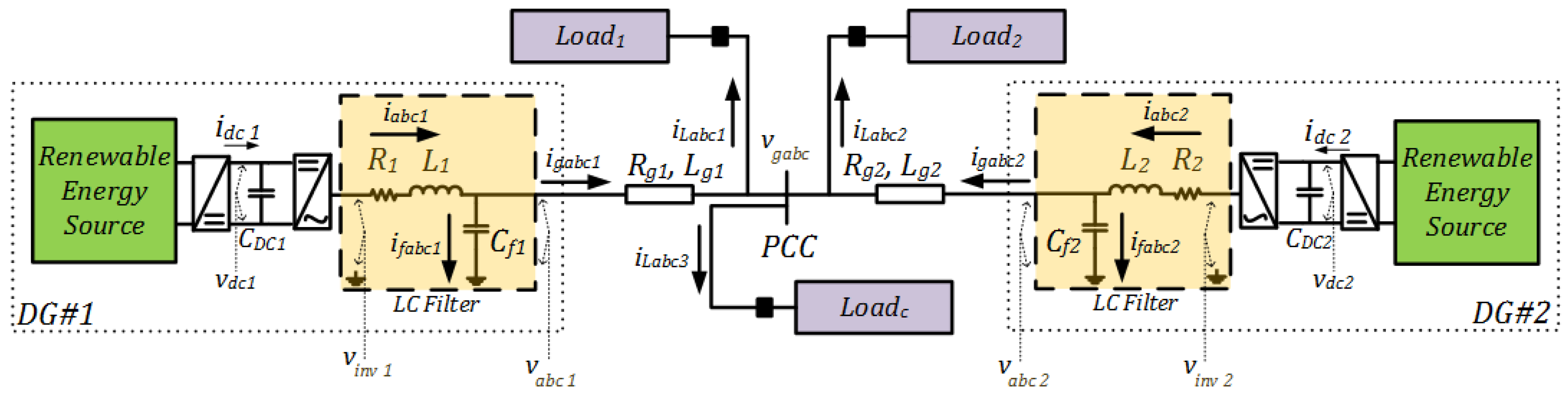
2. Microgrid Model and Analysis

Figure 1 shows the configuration of typical microgrid structure used in this paper. Two DG units are connected to the microgrid with some local or common loads. Based on the derived dynamic model of the system, the steady-state and dynamic analysis will be performed and some new features will be added to primary control level. This model will also be used in the design of the proposed Lyapunov based controller. The dynamic model in the microgrid system is basically written in abc frame [2,6,11]. However, the ability of sine reference tracking largely depends on closed loop bandwidth which may affect the speed of controller as well as undesired significant errors. Thus, the design of a controller in dq rotating frame is a well-known solution in which all variables are DC quantities and the design of controllers is much easier. The dynamic equations can be rewritten in dq rotating frame using the abc/dq transformation [30].

In the islanded MG of Figure 1, each DG unit has a power electronic interface system, LC filter, and control system. The resistance and inductance of coupling transformer and connection cables are included in LC filter parameters. The utilized structure for the inverter is based on well-known three-leg IGBT-based inverter with sinusoidal PWM as described in [30]. After introducing the dynamic model, a thorough analysis is performed to find the capability limitations of each DG and their possible variations which will be used in the proposed control system.

2.1. Dynamic Model of the Microgrid

The Dynamic model of the MG is previously analyzed in [23] and the same equations will be used as follows:

$$L_i\frac{d{i}_{di}}{dt}-\omega L_i{i}_{qi}=-R_i{i}_{di}-u_{di}{v}_{dci}-v_{di},$$

(1)

$$L_i\frac{d{i}_{qi}}{dt}+\omega L_i{i}_{di}=-R_i{i}_{qi}-u_{qi}{v}_{dci}-v_{qi},$$

(2)

$$C_{fi}\frac{d{v}_{di}}{dt}-\omega C_{fi}{v}_{qi}=i_{fdi},$$

(3)

$$C_{fi}\frac{d{v}_{qi}}{dt}+\omega C_{fi}{v}_{di}=i_{fqi},$$

(4)

$$L_{gi}\frac{d{i}_{gdi}}{dt}-\omega L_{gi}{i}_{gqi}=-R_{gi}{i}_{gdi}-v_{di}-v_{gdi},$$

(5)

$$L_{gi}\frac{d{i}_{gqi}}{dt}+\omega L_{gi}{i}_{gdi}=-R_{gi}{i}_{gqi}-v_{qi}-v_{gqi},$$

(6)

$$C_{dci}\frac{d{v}_{dci}}{dt}=u_{di}{i}_{di}+u_{qi}{i}_{qi}+i_{dci}.$$

(7)

The equivalent switching state functions ($u_{ki}$) is used in the voltage equations of AC and DC sides of each DG as follows [23]:

$$v_{inv\_ki}=-u_{ki}.v_{dci}=0.5v_{dci}(s_{ki}-\frac{1}{3}{\displaystyle {\sum }_{k=a}^{b,c}{s}_{ki}}),$$

(8)

where $v_{inv\_ki}$ and $s_{ki}$ are inverter output voltages and its switching functions, respectively.

2.2. Steady-State Capability Curve

In steady-state operation of MG, the system voltages and currents are tend to be kept at the reference values due to the operation of control system. Accordingly, d(.)/dt of these dq variables will be zero. Thus, Equations (1), (2) and (7) can be rewritten in steady-state condition as below:

$$u_{di}^{\ast }=-v_{dci}^{\ast }{}^{-1}(-\omega L_i{i}_{qi}^{\ast }+R_i{i}_{di}^{\ast }+v_{di}^{\ast }),$$

(9)

$$u_{qi}^{\ast }=-v_{dci}^{\ast }{}^{-1}(\omega L_i{i}_{di}^{\ast }+R_i{i}_{qi}^{\ast }).$$

(10)

After some algebraic calculations, the Current-based Steady-state Capability Curve (CSCC) is obtained for each DG unit as below:

$$i_{di}^{\ast }{}^2+i_{qi}^{\ast }{}^2+D{i}_{di}^{\ast }+F=0,$$

(11)

where:

$$D=R_i^{-1}{v}_{di}^{\ast },F=-R_i^{-1}{v}_{dci}^{\ast }{i}_{dci}^{\ast }.$$

Equation (11) is a circle with the center on i^*_d axis and the radius as follows:

$$\left(\begin{array}{c}{c}_{di}^{\ast }\\ c_{qi}^{\ast }\end{array}\right)=\left(\begin{array}{c}-0.5R_i^{-1}{v}_{di}^{\ast }\\ 0\end{array}\right),r_i^{\ast }=\frac{\sqrt{v_{di}^{\ast }{}^2+4R_i{v}_{dci}^{\ast }{i}_{dci}^{\ast }}}{2R_i}.$$

(12)

where $c_{di}^{\ast }$ and $c_{qi}^{\ast }$ are the coordinates of the center and $r_i^{\ast }$ is the radius of the circle.

The CSCC can be used to find capability limits of each inverter-based DG unit to compensate dq components of DG currents. Loads with dq components inside the circle in the first quadrant can be supplied by DG unit in islanding mode of operation. Thus, four important quantities can be obtained as maximum and minimum control limits of currents dq components which will be used in droop-based primary control level:

$$i_{di}^{\ast max}=(\sqrt{v_{di}^{\ast }{}^2+4R_i{v}_{dci}^{\ast }{i}_{dci}^{\ast }}-\left|v_{di}^{\ast }\right|)/(2R_i),$$

(13)

$$i_{qi}^{\ast max}=(\sqrt{v_{di}^{\ast }{}^2+4R_i{v}_{dci}^{\ast }{i}_{dci}^{\ast }})/(2R_i),$$

(14)

$$i_{di}^{\ast min}=(\sqrt{v_{di}^{\ast }{}^2+4R_i{v}_{dci}^{\ast }{i}_{dci}^{\ast }}+\left|v_{di}^{\ast }\right|)/(-2R_i),$$

(15)

$$i_{qi}^{\ast min}=(\sqrt{v_{di}^{\ast }{}^2+4R_i{v}_{dci}^{\ast }{i}_{dci}^{\ast }})/(-2R_i).$$

(16)

Figure 2 shows typical CSCCs for inverter-based DG units in steady state condition. Each DG unit may have its own CSCC due to differences in DG parameters. In this regard, the overlap of the curves (CSCC of MG) and their corresponding maximum and minimum current limits should be considered in the control system design as illustrated in Figure 2. MG operating area which is located in the first quadrant during islanding mode is a relatively smaller limited area which should be considered in reference signal generation.

CSCC center and radius (and therefore its maximum and minimum points) is changed during steady state operation due to possible changes in the parameters. Based on (12), two types of intermittency in the parameters may affect the steady-state circle as explained below:

(1)

Variations of DG interface parameter ($R_i$) (due to ambient temperature, practical operation mismatches and so on);

(2)

AC-side reference voltage ($v_{di}^{\ast }$) variations (generated by droop control level and intermittent generation of renewable energy sources).

In order to study the variations of CSCC and its limits during the above-mentioned variations, the circles are drawn by changing the parameters. It is assumed that the maximum possible change of $R_i$ is equal to ±30%. Voltage variations are also considered to be up to 80% of its nominal value [31]. Figure 3 and Figure 4 show the variations of CSCC to different types of parameter variations.

As it can be seen from these figures, the variations of the parameter $R_i$ do not have a significant effect on the operating area of each DG in the first quadrant while running in steady state. But the effect of $v_{di}^{\ast }$ variations should be noticed. The other noticeable point is the limits of d-component caused by the rating limits of grid conductors along with $i_{di}^{\ast max}$ which can affect the steady state operation area. Other variations in the parameters and variables may occur in dynamic state CSCC which will be discussed in the following section.

2.3. Dynamic-State Capability Curve

In dynamic operation condition, mathematical calculations lead to a circular Current-based Dynamic Capability Curves (CDCC). Considering the instantaneous dynamic variations of AC-side currents as well as DC-link voltage, their time rate of change can be expressed as $\tilde{x}$ = dx/dt, where x is corresponding dynamic current or voltage values.

Equations (1), (2) and (7) can be rewritten in dynamic condition and after some algebraic calculations, the circular CDCC is obtained for each DG unit as below:

$$i_{di}^2+i_{qi}^2+D^{\prime }{i}_{di}+E^{\prime }{i}_{qi}+F^{\prime }=0,$$

(17)

where:

$$\begin{array}{l}{D}^{\prime }=R_i^{-1}(L_i{\tilde{i}}_{di}+v_{di}),E^{\prime }=R_i^{-1}(L_i{\tilde{i}}_{qi}),\\ F^{\prime }=-R_i^{-1}{v}_{dci}(i_{dci}-C_{dci}{\tilde{v}}_{dci}).\end{array}$$

The center and radius of CDCC can be calculated as follows:

$$\begin{array}{l}\left(\begin{array}{c}{c}_{di}^{\prime }\\ c_{qi}^{\prime }\end{array}\right)=\left(\begin{array}{c}-0.5R_i^{-1}(L_i{\tilde{i}}_{di}+v_{di})\\ -0.5R_i^{-1}(L_i{\tilde{i}}_{qi})\end{array}\right),\\ r_i^{\prime }=(0.5R_i^{-1})\times \sqrt{{(L_i{\tilde{i}}_{di}+v_{di})}^2+{(L_i{\tilde{i}}_{qi})}^2+4R_i{v}_{dci}(i_{dci}-C_{dci}{\tilde{v}}_{dci})}.\end{array}$$

(18)

where $c_{di}^{\prime }$ and $c_{qi}^{\prime }$ are the coordinates of the center and $r_i^{\prime }$ is the radius of the circle.

The CDCC is a generalized form of CSCC and can vary dynamically during the operation of the MG. Again, the effective parameters of CDCC dynamic changes can be considered:

(1)

Variations of DG interface parameters ($R_i$ and $L_i$) (due to ambient temperature, practical operation mismatches and so on);

(2)

The amount of dynamic changes of DG variables (${\tilde{i}}_{di}$, ${\tilde{i}}_{qi}$, ${\tilde{v}}_{dci}$) due to changes occurred in loads and generation;

(3)

AC-side voltage ($v_{di}$) variations.

In a dynamic situation, the operating point should be inside a changing CDCC based on the above-mentioned variations. It is also essential that the dynamic trajectory of stable operating points during the occurrence disturbances should be placed inside the CSCC. Another important issue is the square root expression in the CDCC radius equation (${r^{\prime }}_i$) in (18). It is clear that large amounts of $C_{dci}$ at large change rates of $v_{dci}$ may lead to the square root of a negative value which is not an acceptable operating condition.

3. Control System

3.1. Inner Control Loops Based on the Direct Lyapunov Method

The proposed control approach is based on Direct Lyapunov Stability Theory (DLST) [23,32] in a hierarchical structure. The Lyapunov function ($E_L$) for each DG unit is the energy of the system during a dynamic change which can be written as follows:

$$\begin{array}{ll}{E}_L(\Delta i_{di},\Delta i_{qi},\Delta v_{di},\Delta v_{qi},\Delta v_{dci})\hfill & =0.5L_i\Delta i_{di}{}^2+0.5L_i\Delta i_{qi}{}^2+0.5C_{fi}\Delta v_{di}{}^2+0.5C_{fi}\Delta v_{qi}{}^2+\hfill \\ & +0.5L_{gi}\Delta i_{gdi}{}^2+0.5L_{gi}\Delta i_{gqi}{}^2+0.5C_{dci}\Delta v_{dci}{}^2,\hfill \end{array}$$

(19)

where:

$$\begin{array}{l}\Delta i_{dqi}=i_{dqi}-i_{dqi}^{\ast },\Delta v_{dqi}=v_{dqi}-v_{dqi}^{\ast },\\ \Delta i_{gdqi}=i_{gdqi}-i_{gdqi}^{\ast },\Delta v_{dci}=v_{dci}-v_{dci}^{\ast }.\end{array}$$

(20)

Based on Lyapunov theory, the time derivative of the positive Lyapunov function, i.e., (19) should be definitely negative which shows the dissipation of system energy towards zero in the stable operation and its asymptotic global stability. In other words:

$$\begin{array}{cc}{\dot{E}}_L\hfill & =L_i\Delta i_{di}\Delta {\dot{i}}_{di}+L_i\Delta i_{qi}\Delta {\dot{i}}_{qi}+C_{fi}\Delta v_{di}\Delta {\dot{v}}_{di}+C_{fi}\Delta v_{qi}\Delta {\dot{v}}_{qi}+\hfill \\ & +L_{gi}\Delta i_{gdi}\Delta {\dot{i}}_{gdi}+L_{gi}\Delta i_{gqi}\Delta {\dot{i}}_{gqi}+C_{dci}\Delta v_{dci}\Delta {\dot{v}}_{dci}<0.\hfill \end{array}$$

(21)

After some algebraic calculations on (1)–(7) and (20), ${\dot{E}}_L$ can be derived as follows:

$$\begin{array}{cc}{\dot{E}}_L\hfill & =-R_i(\Delta i_{di}{}^2+\Delta i_{qi}{}^2+\Delta i_{gdi}{}^2+\Delta i_{gqi}{}^2)-2(\Delta v_{di}\Delta i_{di}+\Delta v_{qi}\Delta i_{qi})-\hfill \\ & -(\Delta v_{gdi}\Delta i_{gdi}+\Delta v_{gqi}\Delta i_{gqi})-\Delta u_{di}(v_{dci}^{\ast }\Delta i_{di}-\Delta v_{dci}{i}_{di}^{\ast })-\Delta u_{qi}(v_{dci}^{\ast }\Delta i_{qi}-\Delta v_{dci}{i}_{qi}^{\ast })+\hfill \\ & +\Delta v_{dci}\Delta i_{dci}\hfill \end{array}$$

(22)

where:

$$\Delta v_{gdqi}=v_{gdqi}-v_{gdqi}^{\ast },\Delta u_{dqi}=u_{dqi}-u_{dqi}^{\ast }.$$

(23)

In order to have a definitely negative equation in (22), all terms of the equation in the right side must be negative or some of them can be equal to zero. The terms are separated in distinct six terms. The first term is clearly negative. Considering proper regulation around the reference values of voltages by using the proposed controllers ($v_{dqi}\to v_{dqi}^{\ast }$, $v_{gdqi}\to v_{gdqi}^{\ast }$), the next two terms with $\Delta v_{dqi}$ and $\Delta v_{gdqi}$ are zero [2,23]. The 4th and 5th terms are important to derive the dynamic part of the equivalent switching function. By selecting the following expressions for $\Delta u_{dqi}$, the negative value of the corresponding terms in the Lyapunov function will be ensured:

$$\Delta u_{di}=m_{di}(v_{dci}^{\ast }\Delta i_{di}-\Delta v_{dci}{i}_{di}^{\ast })$$

(24)

$$\Delta u_{qi}=m_{qi}(v_{dci}^{\ast }\Delta i_{qi}-\Delta v_{dci}{i}_{qi}^{\ast })$$

(25)

where m_dqi are positive constants.

The steady state part of equivalent switching function ($u_{dqi}^{\ast }$u^*_dqi) was previously proposed in (9) and (10). It can also be proven that the last term ($\Delta v_{dci}\Delta i_{dci}$) in (22) is negative in different operating conditions [23]. The derived Lyapunov-based controller based on stable steady state and dynamic parts of equivalent switching function is shown in Figure 5. The main feature of this controller is considering both AC and DC side changes ensuring the stable operation as well as its integration into a hierarchical structure. The latter will be discussed in the following sections.

The next part of inner control loops in the hierarchical structure is a voltage controller which generates the reference signals for the above-mentioned current controller. A PI controller is used with a feed-forward compensation which is thoroughly discussed in [30].

3.2. Primary Control Level

A droop-based primary controller is responsible for the local voltage reference generation. Two auxiliary approaches are adopted in order to obtain a more accurate voltage reference signal:

(1)

Applying current-based droop equations using fundamental harmonic components and previously calculated limits for each DG unit;

(2)

Harmonics separation of input voltages and currents and then re-adding the separated voltage harmonic parts to the generated reference signal.

To achieve the first approach, the well-known droop equations in fundamental harmonic components are employed that are as the following:

$$\begin{array}{l}{f}_{i1}=f_i^{\ast }-{\alpha }_i(P_{i1}-P_i^{\ast }),\\ v_{i1}=v_i^{\ast }-{\beta }_i(Q_{i1}-Q_i^{\ast }),\end{array}$$

(26)

where $f_{i1}$ and $v_{i1}$ are frequency and voltage magnitude of fundamental harmonic components for the generated reference signal. By assuming the direction of reference vector of voltage in the direction of d-axis (which causes the q-component of voltage to be zero), the output powers of each DG unit in the fundamental frequency can be calculated as:

$$\begin{array}{l}{P}_{i1}=1.5(v_{di1}{i}_{di1}+v_{qi1}{i}_{qi1})=1.5v_{di1}{i}_{di1},\\ Q_{i1}=1.5(-v_{di1}{i}_{qi1}+v_{qi1}{i}_{di1})=-1.5v_{di1}{i}_{qi1}.\end{array}$$

(27)

By substituting (27) in (26), the proposed fundamental dq-current-based droop equations can be obtained as follows:

$$\begin{array}{l}{f}_{i1}={f_i^{\prime }}^{\ast }-{\alpha }_i^{\prime }{i}_{di1},\\ v_{i1}={v_i^{\prime }}^{\ast }+{\beta }_i^{\prime }{i}_{qi1},\end{array}$$

(28)

where:

$$\begin{array}{l}{f_i^{\prime }}^{\ast }=f_i^{\ast }+{\alpha }_i{P}_i^{\ast },{v_i^{\prime }}^{\ast }=v_i^{\ast }+{\beta }_i{Q}_i^{\ast }\\ {\alpha }_i^{\prime }=1.5v_{di1}{\alpha }_i,{\beta }_i^{\prime }=1.5v_{di1}{\alpha }_i\end{array}$$

(29)

Figure 6 shows the droop curves with their corresponding control limits. The limits of dq-currents can be calculated by (13)–(16). The limits for voltage and frequency should also be derived based on a dynamic analysis of droop equations.

The dq-currents in the fundamental frequency can be described by the following equation including steady-state and dynamic-state parts:

$$i_{dqi1}=i_{dqi1}^{\ast }+\Delta i_{dqi1}.$$

(30)

Using (28) and (30), i^*_dqi1 can be derived and substituted in (11) to find the following ellipse:

$$G{f}_i^2+H{f}_i+M{v}_{i1}^2+N{v}_{i1}+K=0,$$

(31)

where the point (f_c, v_c) = (−H/2G, −N/2M) is the center point and (d₁, d₂) = (ρ.x, ρ.y) are the diameters of the ellipse.

They can be calculated as follows:

$$\begin{array}{l}(f_c,v_c)=({f_i^{\prime }}^{\ast }+\Delta f_{i1}+0.5R_i^{-1}{\alpha }_i^{\prime }{v}_{di}^{\ast },{v_i^{\prime }}^{\ast }+\Delta v_{i1}),\\ x={\alpha }_i^{\prime },y={\beta }_i^{\prime },\\ \rho =0.5R_i^{-1}\sqrt{{(v_{di}^{\ast })}^2+4R_i{v}_{D{C}_i}^{\ast }{i}_{D{C}_i}^{\ast }}.\end{array}$$

(32)

Based on this ellipse, the voltage limits of droop curves are as follows:

$$\begin{array}{l}{f}_i^{\ast \max }=f_c+0.5\rho .x,f_i^{\ast \min }=f_c-0.5\rho .x,\\ v_i^{\ast \max }=v_c+0.5\rho .y,v_{i\_\min }^{\ast }=v_c-0.5\rho .y.\end{array}$$

(33)

For the previously mentioned second approach in the primary control, the harmonic separation is applied as follows:

$$v_{dqi}=v_{dqi1}+{\displaystyle {\sum }_{h=2}^n{v}_{dqih}}=v_{dqi1}+(1-LPF)v_{dqi}$$

(34)

where $v_{dqi1}$ and ${\displaystyle \sum v_{dqih}}$ are separated fundamental and other harmonic components, respectively. A low pass filter (LPF) is used to obtain the non-fundamental harmonic components.

3.3. Voltage Intermittency of DC-Side

The intermittent DC power generation in renewable energy sources causes the voltage of the DC-side capacitor to have some variations. The inner Lyapunov-based controller takes the DC-side voltage variations into account, but a complementary controller is used to ensure a stable operating condition. In other words, the reference of the inner current controller should be modified with a proper reference signal generated based on DC-voltage variations as below:

$$i_{di\_ref}=i_{di}^{\ast }+i_{di\_DC}^{\ast }.$$

(35)

The first reference signal ($i_{di}^{\ast }$) is previously generated by inner voltage controller. Considering (7), the second DC component reference signal, $i_{di\_dc}^{\ast }$, can be written as follows:

$$i_{di\_DC}^{\ast }={(u_{di}{v}_{dci})}^{-1}(u_{dci}{v}_{dci}-u_{qi}{i}_{qi}{v}_{dci}-i_{dci}{v}_{dci}),$$

(36)

where $u_{dci}=C_{dci}.d{v}_{dci}/dt$. The AC-side voltage of the inverter ($v_{dqi}$) can be modeled as the product of the switching state function ($u_{di}$ & $u_{qi}$) with the DC-side voltage (v_dci) [24]. On the other hand, by considering d-axis vector in the direction of dq voltage, the q-component of the voltage is zero [34]. Therefore, considering $u_{di}\times v_{dci}\cong v_{di}$ and $u_{qi}\times v_{dci}\cong v_{qi}=0$, Equation (36) can be simplified as follows:

$$i_{di\_DC}^{\ast }={(v_{di})}^{-1}(u_{dci}{v}_{dci}-P_{dci}),$$

(37)

where $P_{dci}=i_{dci}\times v_{dci}$. The control signal $u_{dci}$ can be obtained by a PI compensator ($G_{dc}$ G_dc) with a proper time constant to prevent control interferences:

$$u_{d{c}_i}=k_{pd{c}_i}.(v_{dci}^{\ast }-v_{dci})+k_{id{c}_i}.{\displaystyle \int (v_{dci}^{\ast }-v_{dci})dt}$$

(38)

4. Simulation Results and Discussion

The MG system shown in Figure 1 is utilized to illustrate the effectiveness of the proposed techniques, using MATLAB/SIMULINK. The proposed control system is shown in Figure 7 and the MG parameters are expressed in

Table 1. The parameters of the test system.

Voltage (V)	380	Load#1: RL1 (Ω)	40
Frequency (Hz)	50	Load#1: LL1 (mH)	10
Switching Freq. (kHz)	10	Load#2: RL2 (Ω)	40
DC-side voltage (V)	900	Load#2: LL2 (mH)	10
Ri (Ω)	0.1	Load#3: RL3 (Ω)	40
Li (mH)	45	Load#3: LL3 (mH)	10
Cfi (μF)	200	DG rated active power (kW)	15
Cdci (μF)	2200	DG rated reactive power (kVAr)	10
Lyapunov Coefficient: mdi	10−3	Lyapunov Coefficient: mqi	10−4
Line#1: Rg1 (Ω)	0.02	Line#2: Rg2 (Ω)	0.02
Line#1: Lg1 (mH)	0.024	Line#2: Lg2 (mH)	0.024

. The simulation scenarios are arranged as follows:

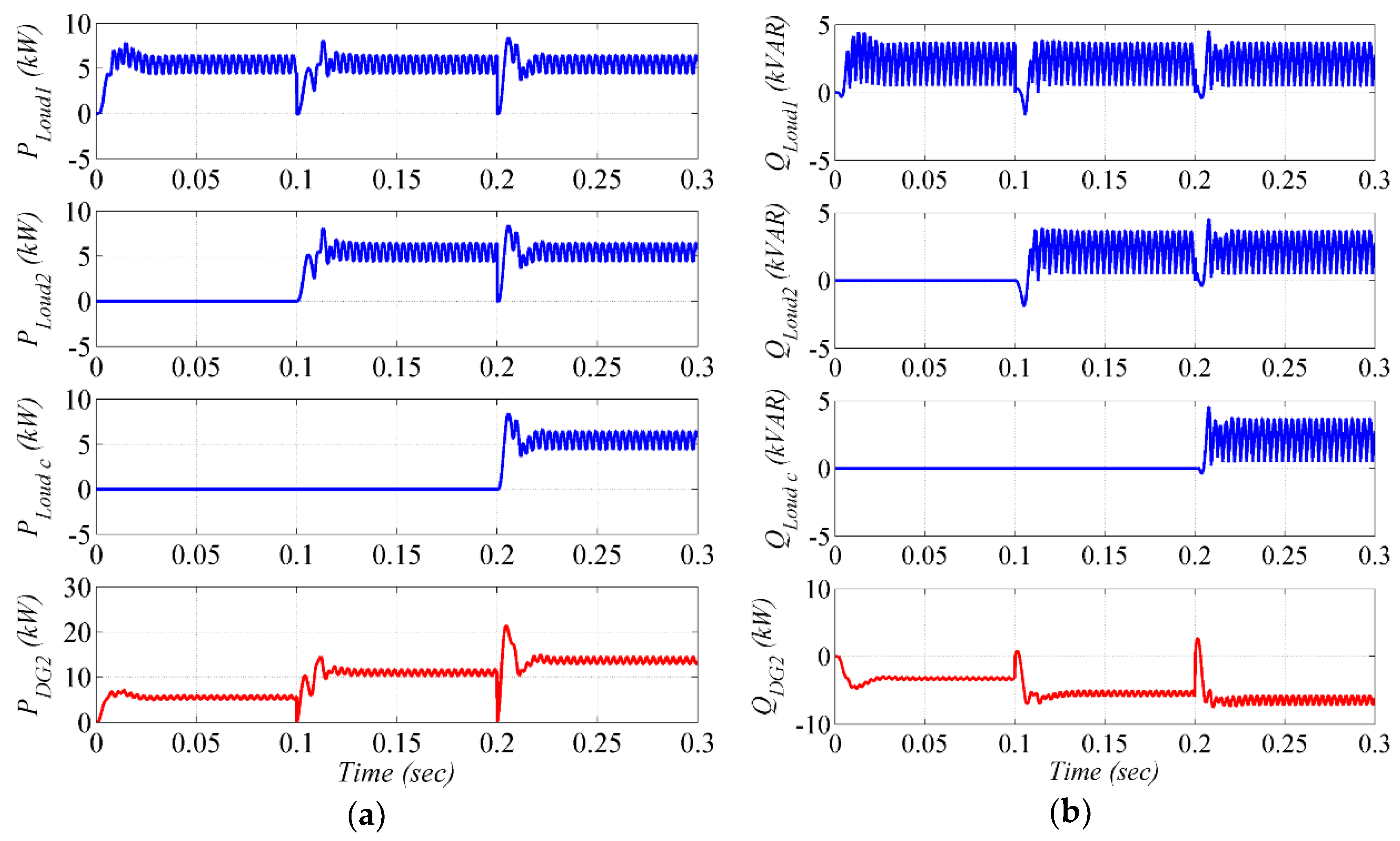
• Steady state operation: Both DG units are supplying local nonlinear loads.
• Local load change: At t = 0.1 s, an additional local nonlinear load is suddenly connected to each DG.
• DC-voltage change: In order to show the effectiveness of the complementary DC-voltage regulation loop, an additional scenario is also considered with a sudden DC-voltage decrease down to 50% of the normal voltage at t = 0.3 s and then a recovery to normal condition at t = 0.5 s. The change takes place after the connection of load#1 at t = 0.1 s.

4.1. Voltage Regulation at Point of Common Coupling

The main goal of the study is the regulation of PCC voltages, which can be seen in Figure 8 and Figure 9. The magnitude and frequency of PCC voltages are maintained in the desired range during sudden changes of loads with small appropriate transients. In this situation, the proposed local control system works properly to adjust the voltage of DG units for different loading conditions. The consideration of the effect of voltage harmonics is an important part to reach these results.

4.2. Voltage Harmonics at Point of Common Coupling

The effectiveness of the harmonic compensation technique used in the proposed multi-purpose control system is investigated in this section. The harmonic contents have been extracted from the measured voltage waveforms using a fast Fourier transform (FFT) analysis in the simulation process.

In Figure 10, the voltage harmonic compensation of the proposed controller can be seen, clearly. The amounts of voltage harmonics are maintained in the desired range based on IEC 61000-2-2 [33] after a major harmonically-distorted load change. The amounts of loads are almost doubled in each change, but the amount of voltage total harmonic distortion is regulated under 5%. In other words, the total harmonic distortion (THD) of voltages is regulated properly by the controller. The harmonic contents of PCC voltages are also illustrated in Figure 10, in which their variations are within the standard range.

4.3. Assessment of Power Sharing

Based on the proposed simulation scenario, the variations of active and reactive powers for each DG unit is assessed in this part. In Figure 11 and Figure 12, the active and reactive powers of DG#1 & 2 along with the loads are illustrated. Each DG unit is able to supply their local loads and also the amount of shared common load. Precisely speaking, the first load change at t = 0.1 s is regulated by the proposed controller with an acceptable transient behavior. The amount of common added load at t = 0.2 s is shared properly between DG units and the corresponding local loads are supplied in a stable way.

Figure 13 shows the above mentioned power variations for DG#2 in one graph to show the power exchange in transient periods and the capability of proper power sharing in the proposed controllers.

4.4. DC-Voltage Variations

It should be noted that the DC-side voltage drop emulates a sudden natural change in renewable energy source of DG units. In order to verify the performance of DC-side voltage loop, after occurrences of a sudden load increase at t = 0.1 s, the DC-side voltage is decreased to 50% of its normal value at t = 0.2 s. Figure 14 shows the effects this scenario on the PCC voltage. As can be seen in Figure 14, the magnitude and frequency of PCC voltages are regulated properly during DC-side voltage variations at t = 0.3 s and t = 0.5 s.

5. Conclusions

In this paper, a modification to the local control of an islanded microgrid is proposed. A direct-Lyapunov-based control scheme is presented for regulating the voltages of a three-phase islanded microgrid in order to ensure the stable operation of the system. The controller is used as an inner local controller for each DG unit and derived based on direct Lyapunov stability theory. The approach of the DLST-based controller in a hierarchical primary control structure along with a DC-side voltage regulator are investigated as the main contribution of this paper. The DLST guarantees the stable operation of each interface converter in the proposed multi-objective control system. In order to have a more accurate reference generation, a current-based droop controller with a voltage harmonic compensation part is used. The control limits of droop equations are calculated by introducing CSCC, CDCC and voltage-frequency ellipse curves. A comprehensive analysis is performed to investigate the effect of some parameters changes on the proposed capability curves. The microgrid steady-state operation area is also obtained. The effectiveness of the designed multi-objective controllers is verified using MATLAB/SIMULINK simulation with harmonically distorted intermittent loads. The results show the appropriate performance of the proposed controllers during both steady-state and transient dynamic conditions.

References

1. Akorede, M.F.; Hizam, H.; Pouresmaeil, E. Distributed energy resources and benefits to the environment. Renew. Sustain. Energy Rev. 2010, 14, 724–734. [Google Scholar] [CrossRef] [Green Version]
2. Mehrasa, M.; Pouresmaeil, E.; Jørgensen, B.N.; Catalão, J.P.S.S. A control plan for the stable operation of microgrids during grid-connected and islanded modes. Electr. Power Syst. Res. 2015, 129, 10–22. [Google Scholar] [CrossRef]
3. IEC 62264-1: Enterprise-Control System Integration—Part 1: Models and Terminology; IEC 62264-1 Standard; International Electrotechnical Commission: Geneva, Switzerland, 2013.
4. IEC 62264-2: Enterprise-Control System Integration—Part 2: Objects and Attributes for Enterprise-Control System Integration; IEC 62264-2 Standard; International Electrotechnical Commission: Geneva, Switzerland, 2015.
5. Milczarek, A.; Malinowski, M.; Guerrero, J.M. Reactive Power Management in Islanded Microgrid—Proportional Power Sharing in Hierarchical Droop Control. IEEE Trans. Smart Grid 2015, 6, 1631–1638. [Google Scholar] [CrossRef]
6. Guerrero, J.M.; Vasquez, J.C.; Matas, J.; Garcia De Vicuna, L.; Castilla, M. Hierarchical Control of Droop-Controlled AC and DC Microgrids; A General Approach Toward Standardization. IEEE Trans. Ind. Electron. 2011, 58, 158–172. [Google Scholar] [CrossRef]
7. Planas, E.; Gil-de-Muro, A.; Andreu, J.; Kortabarria, I.; de Alegría, I.M. General aspects, hierarchical controls and droop methods in microgrids: A review. Renew. Sustain. Energy Rev. 2013, 17, 147–159. [Google Scholar] [CrossRef]
8. Mohamed, Y.A.R.I.; El-Saadany, E.F. Adaptive Decentralized Droop Controller to Preserve Power Sharing Stability of Paralleled Inverters in Distributed Generation Microgrids. IEEE Trans. Power Electron. 2008, 23, 2806–2816. [Google Scholar] [CrossRef]
9. Elrayyah, A.; Cingoz, F.; Sozer, Y. Construction of Nonlinear Droop Relations to Optimize Islanded Microgrid Operation. IEEE Trans. Ind. Appl. 2015, 51, 3404–3413. [Google Scholar] [CrossRef]
10. Hua, H.; Yao, L.; Yao, S.; Mei, S.; Guerrero, J.M. An Improved Droop Control Strategy for Reactive Power Sharing in Islanded Microgrid. IEEE Trans. Power Electron. 2015, 30, 3133–3141. [Google Scholar] [CrossRef]
11. Bidram, A.; Davoudi, A. Hierarchical Structure of Microgrids Control System. IEEE Trans. Smart Grid 2012, 3, 1963–1976. [Google Scholar] [CrossRef]
12. Guerrero, J.M.; De Vicuna, L.G.; Matas, J.; Castilla, M.; Miret, J. A wireless controller to enhance dynamic performance of parallel inverters in distributed generation systems. IEEE Trans. Power Electron. 2004, 19, 1205–1213. [Google Scholar] [CrossRef]
13. De Brabandere, K.; Bolsens, B.; Van den Keybus, J.; Woyte, A.; Driesen, J.; Belmans, R. A Voltage and Frequency Droop Control Method for Parallel Inverters. IEEE Trans. Power Electron. 2007, 22, 1107–1115. [Google Scholar] [CrossRef]
14. Bevrani, H.; Shokoohi, S. An Intelligent Droop Control for Simultaneous Voltage and Frequency Regulation in Islanded Microgrids. IEEE Trans. Smart Grid 2013, 4, 1505–1513. [Google Scholar] [CrossRef]
15. Sefa, I.; Altin, N.; Ozdemir, S.; Kaplan, O. Fuzzy PI controlled inverter for grid interactive renewable energy systems. IET Renew. Power Gener. 2015, 9, 729–738. [Google Scholar] [CrossRef]
16. Logenthiran, T.L.; Naayagi, R.T.; Woo, W.L.; Phan, V.-T.; Abidi, K. Intelligent Control System for Microgrids Using Multi-Agent System. IEEE J. Emerg. Sel. Top. Power Electron. 2015, 3, 1036–1045. [Google Scholar] [CrossRef]
17. Baghaee, H.R.; Mirsalim, M.; Gharehpetian, G.B. Performance Improvement of Multi-DER Microgrid for Small- and Large-Signal Disturbances and Nonlinear Loads: Novel Complementary Control Loop and Fuzzy Controller in a Hierarchical Droop-Based Control Scheme. IEEE Syst. J. 2016, 12, 444–451. [Google Scholar] [CrossRef]
18. Yin, X.; Lin, Y.; Li, W.; Gu, Y.; Liu, H.; Lei, P. A novel fuzzy integral sliding mode current control strategy for maximizing wind power extraction and eliminating voltage harmonics. Energy 2015, 85, 677–686. [Google Scholar] [CrossRef]
19. Xin, H.; Zhao, R.; Zhang, L.; Wang, Z.; Wong, K.P.; Wei, W. A Decentralized Hierarchical Control Structure and Self-Optimizing Control Strategy for F-P Type DGs in Islanded Microgrids. IEEE Trans. Smart Grid 2016, 7, 3–5. [Google Scholar] [CrossRef]
20. Labella, A.; Mestriner, D.; Procopio, R.; Brignone, M. A new method to evaluate the stability of a droop controlled micro grid. In Proceedings of the 2017 10th International Symposium on Advanced Topics in Electrical Engineering (ATEE), Bucharest, Romania, 23–15 March 2017; pp. 448–453. [Google Scholar]
21. Rocabert, J.; Luna, A.; Blaabjerg, F.; Rodriguez, P. Control of Power Converters in AC Microgrids. IEEE Trans. Power Electron. 2012, 27, 4734–4749. [Google Scholar] [CrossRef]
22. Rasheduzzaman, M.; Mueller, J.A.; Kimball, J.W. An Accurate Small-Signal Model of Inverter- Dominated Islanded Microgrids Using dq Reference Frame. IEEE J. Emerg. Sel. Top. Power Electron. 2014, 2, 1070–1080. [Google Scholar] [CrossRef]
23. Pouresmaeil, E.; Mehrasa, M.; Catalao, J.P.S. A Multifunction Control Strategy for the Stable Operation of DG Units in Smart Grids. IEEE Trans. Smart Grid 2015, 6, 598–607. [Google Scholar] [CrossRef]
24. Mehrasa, M.; Pouresmaeil, E.; Catalao, J.P.S. Direct Lyapunov Control Technique for the Stable Operation of Multilevel Converter-Based Distributed Generation in Power Grid. IEEE J. Emerg. Sel. Top. Power Electron. 2014, 2, 931–941. [Google Scholar] [CrossRef]
25. Mehrasa, M.; Pouresmaeil, E.; Akorede, M.F.; Jørgensen, B.N.; Catalão, J.P.S. Multilevel converter control approach of active power filter for harmonics elimination in electric grids. Energy 2015, 84, 722–731. [Google Scholar] [CrossRef]
26. Hoseini, S.K.; Pouresmaeil, E.; Hosseinnia, S.H.; Catalão, J.P.S. A control approach for the operation of DG units under variations of interfacing impedance in grid-connected mode. Int. J. Electr. Power Energy Syst. 2016, 74, 1–8. [Google Scholar] [CrossRef]
27. Mehrasa, M.; Pouresmaeil, E.; Zabihi, S.; Catalão, J.P.S. Dynamic model, control and stability analysis of mmc in HVDC transmission systems. IEEE Trans. Power Deliv. 2017, 32, 1471–1482. [Google Scholar] [CrossRef]
28. Mehrasa, M.; Pouresmaeil, E.; Zabihi, S.; Rodrigues, E.M.G.; Catalão, J.P.S. A control strategy for the stable operation of shunt active power filters in power grids. Energy 2016, 96, 325–334. [Google Scholar] [CrossRef]
29. Mehrasa, M.; Pouresmaeil, E.; Mehrjerdi, H.; Jørgensen, B.N.; Catalão, J.P.S. Control technique for enhancing the stable operation of distributed generation units within a microgrid. Energy Convers. Manag. 2015, 97, 362–373. [Google Scholar] [CrossRef]
30. Yazdani, A.; Iravani, R. Voltage-Sourced Converters in Power Systems: Modeling, Control, and Applications; John Wiley & Sons: Hoboken, NJ, USA, 2010; ISBN 0470551569. [Google Scholar]
31. Mahmud, M.A.; Hossain, M.J.; Pota, H.R.; Oo, A.M.T. Robust Nonlinear Distributed Controller Design for Active and Reactive Power Sharing in Islanded Microgrids. IEEE Trans. Energy Convers. 2014, 29, 893–903. [Google Scholar] [CrossRef]
32. Dasgupta, S.; Mohan, S.N.; Sahoo, S.K.; Panda, S.K. Lyapunov Function-Based Current Controller to Control Active and Reactive Power Flow From a Renewable Energy Source to a Generalized Three-Phase Microgrid System. IEEE Trans. Ind. Electron. 2013, 60, 799–813. [Google Scholar] [CrossRef]
33. IEC 61000-2-2: Electromagnetic Compatibility (EMC)—Part 2-2: Environment—Compatibility Levels for Low-Frequency Conducted Disturbances and Signalling in Public Low-Voltage Power Supply Systems; IEC 61000-2-2; International Electrotechnical Commission: Geneva, Switzerland, 2002.
34. Pouresmaeil, E.; Miguel-Espinar, C.; Massot-Campos, M.; Montesinos-Miracle, D.; Gomis-Bellmunt, O. A Control Technique for Integration of DG Units to the Electrical Networks. IEEE Trans. Ind. Electron. 2013, 60, 2881–2893. [Google Scholar] [CrossRef]
Figure 1. Single-line diagram of the studied microgrid.
Energies 11 01161 g001
Figure 2. CSCC for each DG unit of the MG: typical CSCC and the limits of currents along with the overlap of CSCCs for different DG units and reference current area of MG.
Energies 11 01161 g002
Figure 3. Variation of CSCC due to variations of Ri.
Energies 11 01161 g003
Figure 4. Variation of CSCC due to variations of v*di.
Energies 11 01161 g004
Figure 5. The block diagram of the proposed Lyapunov-based inner controller.
Energies 11 01161 g005
Figure 6. Droop curves of primary control level based on dq-currents.
Energies 11 01161 g006
Figure 7. Hierarchical local controllers of each DG unit with a Lyapunov-based control loop.
Energies 11 01161 g007
Figure 8. The waveform of the voltages at PCC.
Energies 11 01161 g008
Figure 9. (a) Magnitude and (b) frequency variations of phase voltages at PCC.
Energies 11 01161 g009
Figure 10. The variations of THDv levels and harmonic contents for PCC voltages during load changes: (a) t = 0~0.1, (b) t = 0.1~0.2, (c) t = 0.2~0.3.
Energies 11 01161 g010
Figure 11. The Variations of Active and Reactive powers for DG#1 and the loads: (a) active power; (b) reactive power.
Energies 11 01161 g011
Figure 12. The Variations of Active and Reactive powers for DG#2 and the loads: (a) active power; (b) reactive power.
Energies 11 01161 g012
Figure 13. The Variations of (a) Active and (b) Reactive powers for DG#2 and the loads.
Energies 11 01161 g013
Figure 14. (a) Magnitude and (b) frequency variations of phase voltages at PCC during DC-side voltage variations.
Energies 11 01161 g014