Abstract
Distributed PV power generation necessitates both intra-hour and day-ahead forecasting of solar irradiance. The UTSA SkyImager is an inexpensive all-sky imaging system built using a Raspberry Pi computer with camera. Reconfigurable for different operational environments, it has been deployed at the National Renewable Energy Laboratory (NREL), Joint Base San Antonio, and two locations in the Canary Islands. The original design used optical flow to extrapolate cloud positions, followed by ray-tracing to predict shadow locations on solar panels. The latter problem is mathematically ill-posed. This paper details an alternative strategy that uses artificial intelligence (AI) to forecast irradiance directly from an extracted subimage surrounding the sun. Several different AI models are compared including Deep Learning and Gradient Boosted Trees. Results and error metrics are presented for a total of 147 days of NREL data collected during the period from October 2015 to May 2016.
1. Introduction
For photovoltaic (PV) generation to achieve increased penetration into the world’s electric grid, there is a pressing need for high-accuracy Global Horizontal Irradiance (GHI) forecasts [1]. Occasioned by a cloud moving between the PV array and the sun, a ramp event may last for only several minutes, but results in a sudden large drop in power output. If it is known in advance that a ramp event will occur, then the utility can take corrective action. Intelligent control of the active/reactive power in solar panel inverters during ramps will permit frequency regulation and load management as well as provide a failsafe mechanism during cascading grid outages. The energy alliance between the University of Texas at San Antonio (UTSA) and the municipal electric utility CPS Energy has the goal of developing new technologies that combine inexpensive all-sky imaging cameras with sophisticated image processing techniques, and now artificial intelligence software, to achieve highly accurate 15 min ahead GHI predictions. Previous work [2,3] describes the UTSA SkyImager. For a historical survey of solar irradiance and PV power forecasting, see the recent article [4].
GHI consists of two components, the Direct Normal Irradiance (DNI) and the Diffuse Horizontal Irradiance (DHI): where is the zenith angle. Cloud shadows significantly impact DNI, whereas they have little effect upon the background DHI that is caused by secondary reflections and re-radiation. Figure 1 displays the three quantities GHI, DNI, and DHI, for 27 October 2015 at the National Renewable Energy Laboratory (NREL) and shows that moderately cloudy conditions can cause multiple ramp events. How well does the GHI time series correlate with the UTSA SkyImager [2] pictures? Figure 2 displays a sequence of eight pictures taken by the SkyImager at the NREL site, one every 2 min starting (upper left) at 12:31 p.m. MST. At that time, the sun is not obscured, but cumulus clouds are moving in from the left. At 12:35, the cloud begins to enter the solar disk and, by 12:37, the sun is completely occluded. This continues until 12:42, when the cloud has moved past the sun and the DNI recovers. While this example considers a single ramp event, the strong correlation between measured GHI and the presence of clouds obscuring the sun in the SkyImager pictures suggests that AI models would be very successful at learning this functional relationship.
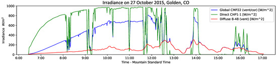
Figure 1.
Measured GHI (blue), DNI (green), and DHI (red) in units of W/m for 27 October 2015 versus Mountain Standard Time in hours. The ramp event displayed in Figure 2 is seen in the DNI oscillations that occur around noon.
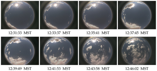
Figure 2.
An image sequence recorded on 27 October 2015 at Golden, CO. Beginning (upper left) at 12:31 p.m. and ending (lower right) at 12:46 p.m., there are 2 min between each image. A cloud obscuring the sun results in a large ramp event.
2. Materials and Methods
The basic problem to be addressed in short-term solar forecasting is: “Where will shadows of low clouds be fifteen minutes in the future?” These shadows cause precipitous rises and falls in power produced by solar panels. Our approach takes into account as much of the physics as possible, but is an idealization necessitated by the need to produce GHI forecasts in real time for a micro-grid management system. Solving the Navier–Stokes equations to take into account the true dynamics of the atmosphere is not feasible on a Raspberry Pi and probably unnecessary for this problem.
2.1. UTSA SkyImager
Several previous papers [2,3,5,6] have detailed the development and deployment of the low cost, edge-computing UTSA SkyImager (Patent Pending). Figure 3 shows the SkyImager deployed at four locations: NREL in Golden, CO, Joint Base San Antonio, and two locations in the Canary Islands. A security camera enclosure houses a Raspberry Pi computer with programmable digital camera. In the configuration used for this study with NREL data, several external inputs were required for our algorithms: distortion parameters for the fish eye lens, zenith angle, True North, and finally the cloud base height (CBH). A sequence of image processing transformations is applied to each of the fused pictures taken by the Pi camera, as described in detail in [2]. For completeness, a brief summary of the pipeline is included here: (1) removal of the fish eye lens distortion; (2) cropping and masking; (3) calculation of the “Red-to-Blue Ratio” (RBR); (4) application of a median filter to remove impulsive noise; (5) Thresholding to determine cloud presence; (6) computing cloud cover percentage and deciding clear/moderately cloudy/overcast; (7) projecting cloud locations to a height equal to CBH; (8) optical flow; (9) ray-tracing to locate cloud shadows; and (10) calculating GHI values using shadow locations. Although physically correct, Step (9) ray-tracing falls in the category of an inverse problem and, as stated in [3], is “ill-posed”. To circumvent this issue, it was decided to investigate the use of artificial intelligence and neural works to forecast GHI values directly from the predicted cloud locations.
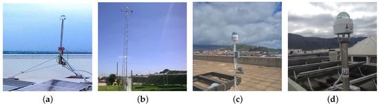
Figure 3.
The UTSA SkyImager deployed at: (a) the ESIF building at the National Renewable Energy Laboratory (NREL); (b) the microgrid at the Joint Base San Antonio; (c) Tenerife, Canary Islands; and (d) Caleta de Sebo, on La Grasiosa.
2.2. Optical Flow
In a video sequence, the pattern of brightness appears to move through the field of view. This optical flow can result from moving objects or the camera panning. Given the intensity value at pixel location , one needs to determine the component of the velocity of E, and, similarly the component of the velocity . Enforcing the optical flow constraint: , does not necessarily give a unique solution. A penalty term must be incorporated to ensure the solution is smooth except at edges. The energy functional in the variational formulation has two terms: and . Minimizing gives the Euler equations.
Computationally expensive, calculating requires reduction in dimensionality to be effective [7]. A sparse set of features is extracted from each image—say the corners of objects appearing in the picture. The Lucas–Kanade algorithm [8] is implemented in the OpenCV open computer vision software package and the results shown in Figure 4. White dots show the predicted corner locations five, ten, and fifteen minutes from the current time. This knowledge can then be used to calculate centroids of cloud masses and advect the entire cloud into the future.
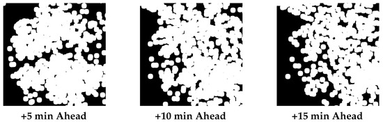
Figure 4.
Using OpenCV’s optical flow algorithm to predict corner locations at 11:13 a.m. for 23 October 2015.
2.3. Machine Learning
Shadows cast by cumulus clouds cause a sudden, significant decrease in GHI and the attendant drop in power generation. The complicated functional relationship between shadow locations and irradiance values can be “learned” by neural networks (NN). If cloud locations are accurately forecasted using optical flow, then this relationship can be exploited to give accurate GHI predictions. Indeed, machine learning has been used for several years in solar forecasting [9,10,11] and many other areas of sustainable energy [12,13,14].
Neural Networks seek brain-like functionality by combining large numbers of very simple artificial neurons. As detailed below, a nonlinear activation function acts on a weighted sum of inputs and above a certain threshold the neuron “fires”. Neurons are organized into layers with output of one layer “feeding into” the next layer as input. At a high level, there are two phases of machine learning or artificial intelligence: training or learning and inference or prediction. The analogy with human learning is clear and similar terminology exists in both disciplines. With the large number of machine learning (ML) models available, it was prudent to concentrate on those that we felt would achieve the best results for our problem. Table 1 shows a taxonomy of machine learning. This paper focuses on Deep Learning and Gradient Boosted Trees.

Table 1.
Taxonomy of machine learning.
2.4. Multi-Layer Perceptrons and Deep Learning
Artificial neural networks have evolved greatly since Rosenblatt proposed the perceptron, but the latter provides a good starting point for explaining today’s sophisticated Deep Learning (DL) architectures. In a simple feed-forward network, a vector of length m representing one example in a data set containing perhaps 100,000 samples (called examples) is input to the network. Figure 5a shows that a weighted sum of the inputs is then calculated, and an inner product is computed . This dot product becomes the argument to an “activation” function that serves as a threshold to determine when the neuron fires [15]. Many choices for are possible: the Heaviside step function, a linear function, or a sigmoid function such as . The goal of supervised learning is to find those weights that give the best agreement between the actual target classes and those predicted using the given weights. The optimization problem is often solved iteratively using gradient descent [16]. Effective on the binary classification problem, the approach can be expanded for multiple classes or the continuous output (regression) problem.
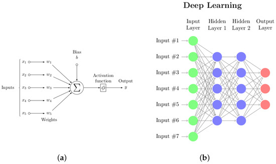
Figure 5.
(a) Schematic of a perceptron with a single binary output; and (b) a multi-layer perceptron with two hidden layers. It is represented by a directed graph in which information flows from left to right. Both the number of hidden layers and the number of nodes in each layer can be varied. Most researchers agree that a credit assignment path (CAP) depth—# hidden layers plus 1, value of >2 constitutes “deep learning”.
In a Multi-Layer Perceptron (MLP), there are one or more hidden layers between the input and output layers. The increased number of connections mimics biological networks [17] and allows for a much richer learning of information patterns in the data. In Figure 5b, each neuron in Hidden Layer 1 (HL1) is connected to all the input nodes (full connectivity); in addition, each neuron in HL1 is connected to all nodes in Hidden Layer 2 (HL2). The topology of the MLP is represented by a directed graph in which information flows from left to right (feed-forward). Finally, the outputs from HL2 become the inputs for the Output Layer which represents three classes. Denoting an input example by , organizing the weights between Input and HL1 into a matrix , and defining a vector function which applies the scalar function component-wise, the output from Layer 1 is . This becomes the input to Layer 2 where a weight matrix is applied to yield . Applying a final weight matrix gives the output . As with a perceptron, the weights are chosen to minimize the discrepancies between the actual and predicted labels. Back-propagation is a particularly effective strategy for optimizing the weights: stochastic gradient descent can be used to avoid becoming trapped in a local valley.
In his historical overview, Schmidhuber [18] distinguished between “Shallow” and “Deep” learning in a MLP using a credit assignment path (CAP) depth, which is the number of hidden layers plus one (for the parameterized output layer). A CAP depth of 2 yields a universal approximator that can represent any function, beyond that extra layers learn features and “causal links between actions and effects”. For this reason, a working definition of “Deep” learning is often taken to be a CAP depth greater than 2. The reader interested in learning more about deep learning should consult References [19,20,21].
While the choice of an optimization strategy can be critical for implementation, problem formulation as a neural network is independent of this choice. Evolutionary or genetic methods for optimizing nondifferentiable objective functions can be employed effectively. In fact, these methods are connected with the decision trees discussed next. Implicitly or explicitly, every approach to machine learning involves optimization of a cost/loss/energy/objective functional and in deep learning one seeks the optimal weights w. A standard strategy for minimizing a functional J is steepest descent which moves from the current approximation to a new one in the direction of the negative gradient: . In practice, a more refined algorithm uses a stepsize or “learning rate” with momentum and or regularization which adds a penalty term or to reduce overfitting. This gives the modified loss functional in Equation (3) and general descent algorithm shown in Equation (4),
where y is the actual target value and is the predicted value with current weights w. There are several “tunable” parameters associated with MLP and deep learning software that are summarized in Table 2. Carefully choosing these parameters can significantly improve convergence of the algorithms and decrease errors.
Table 2.
Deep learning parameters. (Name refers to the parameter name in the software.)
2.5. Decision Trees and Random Forests
Decision trees are popular machine learning models for classification and regression. As the name suggests, the method uses the input data to recursively build a rooted tree in which the top vertex is designated the root and there is a unique path to every vertex directed away from the root. Starting at the root with all the data in one class, a decision is made to split the data into two subclasses using the feature that results in the largest information gain defined as
where f denotes a feature; and are the datasets of the parent and j-th child node, respectively; and and are the number of samples of the parent and j-th child node, respectively. In a binary decision tree, j is either or . Three common splitting criteria for the impurity measure I in Equation (5) are entropy, Gini impurity, and classification error. Decision trees can build complex boundaries in feature space, but care must be exercised to avoid overfitting of the data. Random forests [22] are an example of ensemble learning, which combines weak learners for robustness and strong learners to reduce overfitting and generalization error. The algorithm can be summarized as: (1) draw bootstrap sample of size n; (2) grow a decision tree from bootstrap sample; (3) repeat Steps (1) and (2) k times; and (4) aggregate prediction by each tree to assign class labels by majority vote. The Gradient Boosted Trees algorithm in RapidMiner uses stochastic gradient descent to improve the convergence properties of this random forests algorithm. Figure 6 shows part of the decision tree by this applied to the NREL dataset.
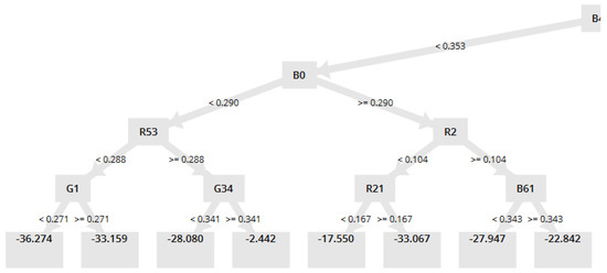
Figure 6.
Part of the decision tree output by the Gradient Boosted Trees algorithm for the NREL data.
AI software for data mining of massive datasets has evolved quickly over the last few years. Rapidminer (RapidMiner USA, Boston, MA, USA) [23] is a machine learning platform with a point and click interface, convenient import/export of datasets, and a multitude of AI models. In several cases, it utilizes the HO (Version 3.8.2.6, HO.ai, Mountain View, CA, USA) [24,25,26] machine learning modules. Specifically, our DL model is found in HO as the python function HODeepLearningEstimator(). Scikit-Learn (scikit-learn.org) [27] is an open source Python package that allows a user to prototype and compare a variety of classification, clustering, and regression models. Neural networks and deep learning have seen the evolution of specialized software such as Keras, Theano, and Google’s Tensorflow which recently became open source. The computational demands of training networks on big data are extreme and this has resulted in a hardware evolution from central processing units (CPU) to graphical processing units (GPU) to special purpose tensor processing units (TPU).
3. Results and Discussion
Before examining the results for various machine learning models in terms of accuracies, it is important to precisely state the problem we have solved. The ultimate goal is intra-hour GHI and PV power predictions in real time, but those forecasts are the result of a two-step process: predicting where low level cumulus clouds will be 15 min ahead in time and then using projected cloud locations to accurately predict the GHI. Each step introduces errors. A brief introduction to the optical flow problem for the SkyImager is presented above. Work is currently in progress to determine the accuracies for Step 1: compute error metrics of the 15 min ahead predicted image minus the actual image. It will be the subject of a future article. Step 2 will take the predicted image and compute the GHI using machine learning as discussed in this paper. There are several benefits to this approach. It separates the optical flow component from the machine learning, and, more importantly, it allows GHI to be predicted directly from the image itself so that the Pi camera can become a tool for measuring/observing GHI.
Each input or “example” is a three-channel image from the Pi camera. In the current configuration, three images taken 5 s apart at low, medium, and high exposure times are fused using the Mertens algorithm into one raw image. As mentioned, this approach reduces over-exposure and washout in the circumsolar region. The pixel JPEG image forms the basic input measurement for both the optical flow and machine learning algorithms. Low level cumulus clouds between the sun and the PV arrays have the greatest effect on the DNI, hence on GHI. For that reason and to satisfy the need for dimensionality reduction [28], the first preprocessing step is to locate the area in the image that surrounds the sun and extract a pixel subimage. Several approaches to locating the sun in the image are possible. Calculating the zenith angle from the SOLPOS program, finding true North, and then mapping physical to pixel coordinates would require extensive calibration. It was decided to use a simple robust image processing approach that finds the maximum intensity in the image. On a clear day, this always locates the sun, but occasionally, when the sun is totally obscured by broken clouds, the brightest point in the picture is actually sunlight reflected off of a nearby cloud. This can be observed in a time lapse video clip in which for a few frames the sun is not at the center of the subimage. While the cause of some transient errors, it never lasts long and does not happen when the sun is totally obscured by a uniform cloud deck without breaks. Figure 7a shows the low exposure image used to locate and center the sun and Figure 7b the resulting raw fused image that will ultimately become the input to the neural networks. Lastly, the subimage is resized to a point () where the neural networks can be trained in a reasonable amount of time. In supervised learning, the neural networks require labeled training examples: ordered pairs where x is the input vector, in this case the extracted subimage , and y is the measured irradiance in units of Watts/m at the time the picture was taken. Since new images are fused every 15 s, GHI values were treated as constant on a 60 s interval for the purposes of assigning labels for the neural network images.
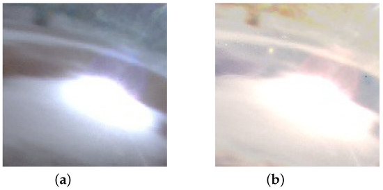
Figure 7.
Subimages of circumsolar region: (a) a low exposure image taken on 18 November 2015 at 9:00 MST; and (b) the raw image fused from low, medium, and high-exposure images. This pixel subimage captures that portion of the large image that most directly affects the GHI.
Forecasting GHI on a clear day, , is effectively solved by several available models [29], e.g., the Haurwitz model: , where is the solar zenith angle. The presence of clouds alone will cause measured GHI to depart from the clear sky , so that the latter could be used as an additional input feature for machine learning if desired. The networks would not have to “learn” the functional dependence on . Many other statistics derived from the basic image data could also be used for training. In addition, a better target than GHI might be the value , the deviation from the clear sky value.
The above details are critical to precisely define the inputs to the neural networks and to ensure reproducibility of our results. Equally important is a detailed understanding of the metrics that appear in Table 3. These are used to evaluate models and ultimately provide the utility with error bounds for making economic decisions. MAPE is a standard metric for evaluating the performance of irradiance forecasting algorithms. Problems in its use can occur when is zero or very small. As an alternative, the mean of the actual values is often used in the denominator, as is common practice when forecasting spot electricity prices. Note that MAPE is the relative error in the metric, normalized for the number of observations, and converted to a percentage. In the field of machine learning, there are standard ways of visualizing both the input dataset consisting of vectors in a high dimensional space, as well as targets and predicted outputs.
Table 3.
Regression Metrics: A actual, F forecast, and mean.
All images were collected by the UTSA SkyImager (UT Board of Regents, Austin, TX, USA) deployed on the rooftop of the ESIF building at the NREL in Golden, Colorado. This was part of the Department of Energy INTEGRATE project. Observations began in October 2015 and continued until May 2016. During this period of 147 days, there were 14 days of no data collected for technical reasons and 27 days of only partial data collection (omitted in our analysis), leaving 106 days of no missing data. These formed the inputs for training and testing the neural networks. The dataset containing 106 days yield observations (examples or rows) for input to the networks. With the standard 70%:30% split into training and testing subsets, examples were used for training and used for testing.
Each example represents an image taken at a particular time of a day, and includes the RGB normalized pixel values of a resized subimage centered about the sun. The resizing was necessary for dimensionality reduction and runtimes, but work is underway to rerun the software in a distributed environment with the subimages themselves. In addition, the average values of each of the three channels are included as additional features, giving a total of features. Finally, column-0 in the input data matrix is the measured GHI value at that time in .
A standard way of showing how well random variables X and Y are correlated is with a scatter diagram. Scatterplot matrices display pair-wise correlations between different features in the dataset, but, in the case of images with RGB pixel values, the number of features renders this approach less valuable than it is with the Boston housing dataset, for instance. Figure 8 shows scatter diagrams of measured GHI versus predicted GHI for several different machine learning models: Multi-Layer Perceptron (MLP), Random Forest (RF), Deep Learning (DL), and Gradient Boosted Trees (GBT). A quick inspection shows that, while all four models perform well with tight clustering around the line (perfect correlation), there are differences. The DL and GBT models have fewer outliers and visually outperform the other two models, but a more quantitative assessment is needed.
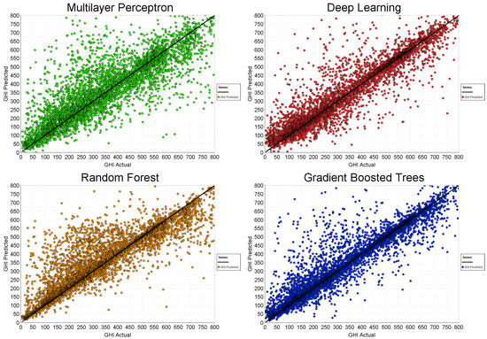
Figure 8.
GHI actual (measured) vs. GHI predicted for 24 October 2015 using several different AI models.
It is important to note that the first two models, MLP and RF, were run on the Scikit-Learn platform while the results of the second two models, DL and GBT, are from Rapidminer. This was done intentionally for several reasons. First, to validate our results on different machine learning platforms, model results should depend on the algorithm used not the platform on which they are implemented. Scikit-Learn does not currently implement a deep learning model in their standard suite of ML models. While Rapidminer is very convenient to use on a PC, ultimately, our goal is to take the weights determined by the training process and use them in real time on a Raspberry Pi 3 computer (Raspberry Pi Foundation, Cambridge, UK) where the Scikit-Learn platform with its open source python interface should prove easy to use.
Table 4 gives detailed error metics, i.e. MAE, MAPE, nRMSE, and R values, as well as the run times. Perhaps most significant is the explained variance—the R value in the last column. It shows that both DL and GBT models achieve a value in the range of , while MLP and RF have values which are less. (A perfect correlation would have R equal 1). The other error metrics track the R values. The extra accuracy is bought at the expense of significantly longer run times in the case of deep learning, but the hybrid GBT model actually achieves the highest accuracy with a very fast runtime, 10 min faster than generic random forests.
Table 4.
Evaluation of four machine learning models.
In this case, a second approach to displaying and understanding our results is a time series, in which predicted or measured GHI values are plotted on the y-axis as a function of time, plotted on the x-axis. Zooming in on one day of data, Figure 9 compares measured and predicted GHI for 3 October 2015. At this scale, there are differences mainly because this is an overcast day that makes prediction more difficult, but in overall trend the two curves track each other well.
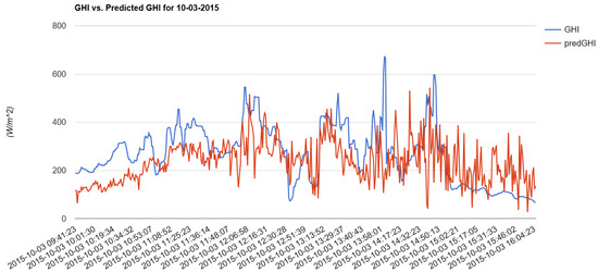
Figure 9.
Measured GHI (blue) vs. predicted GHI (red) for an overcast day—3 October 2015.
More illuminating is a time series graph of measured versus predicted GHI for the entire testing dataset, as shown in Figure 10. Once again, actual GHI is in blue and the forecast values are in red. Because the two curves track each other so closely, it is difficult at times to tell them apart. Both figures used the DL model to predict the target GHI values. In the middle of the graph, one can see a string of five consecutive clear sky days which are relatively easy to predict. In other places, overcast days are evident, and on moderately cloudy days the two curves differ most.
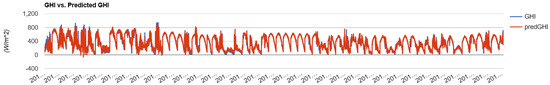
Figure 10.
Measured GHI vs. predicted GHI for all days in the test dataset.
It is instructive to examine a detailed Rapidminer plot of the output for the GBT model. Figure 11 displays the predicted GHI in W/m as a function of time on the x-axis for those days in the testing data. It is straightforward to determine clear sky days (see the six days in the middle of the plot), as well as moderately cloudy days with numerous ramp events. Decision trees were introduced earlier. They predict an outcome by “splitting” the input examples using multiple conditional statements, yielding a tree-like structure that allows for easy identification of the most important features. Ensembles of decision trees can suffer from high variance, however. The gradient boosting improves overall accuracy by building a network of trees using a feature importance statistic which indicates the most influential features—those which decrease MSE values most during splitting. There is no final decision tree and interpreting the results is not as straightforward as in the case of RF. As our results show, GBTs are competitive with deep learning accuracies on the GHI forecasting problem, with significantly smaller run times.
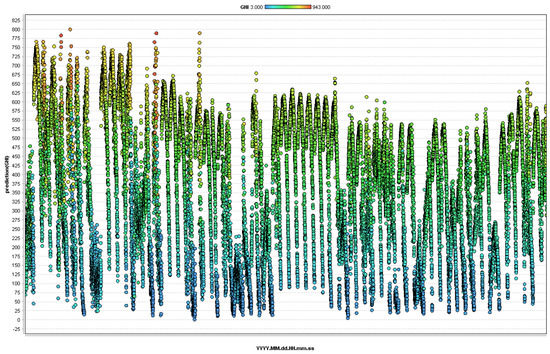
Figure 11.
Rapidminer plot of the predicted GHI (W/m) as a function of time () using their Gradient Boosted Trees model for all days in the test dataset and the weights determined with the training data.
As mentioned, there are many parameters for each of the models that can be tuned to optimize accuracies and run times. Table 5 shows for the DL model how changing the number of hidden layers and nodes in those layers, and varying the number of epochs (one complete pass through the entire training dataset) affects the results. Model 1 has two hidden layers with 50 nodes in each and uses only ten epochs to achieve R = 0.815 with a run time of just under 2 min. Model 2 with two hidden layers (195, 195) and the same 10 epochs takes over three times as long and only improves the value of R to 0.824. To get a value of 0.871, Model 3 (195, 195, 195) requires 500 epochs and almost 45 min to run, while Model 4 (195, 195, 97, 195, 195) takes over an hour to run on a desktop PC. A point of diminishing returns has been reached—probably with Model 2—and further improvements in accuracy would be achieved by using larger images or tuning other deep learning parameters.
Table 5.
Comparison of four deep learning models.
4. Conclusions and Ongoing Research
The problem of predicting GHI 15 min ahead can be separated into several distinct sub-problems. (1) Acquiring a time-sequence all-sky images includes taking multiple images at different exposure times and fusing them to produce one raw image every 15 s. (2) This time sequence and an optical flow algorithm are used to move clouds 15 min ahead in time. For this step, full pixel images are necessary for accurately forecasting cloud locations. A future paper will address optical flow in detail, but several comments are in order. Clouds occur at multiple levels in the atmosphere with the standard METAR classification being low, middle, and high clouds. Our methodology, which focuses on cumulus clouds, is a first-order approximation. Refinements are possible, but must do not interfere with the system’s ability to produce predictions in real time. (3) Finally, using the predicted image, a forecast of GHI is produced. Ray-tracing was used in the original implementation to predict the presence of cloud shadows over the PV arrays. This problem is ill-posed, so small errors in shadow locations can potentially lead to large errors in GHI. Our current work demonstrates that, by extracting a pixel subimage from the circumsolar region of the 15 min ahead predicted image and applying machine learning, it is possible to accurately forecast GHI values. Training the networks offline can be expensive and we are looking at Tensorflow. However, once the optimal weights have been found, the calculation of one predicted GHI value is very fast—it just amounts to taking an inner product. The possible bottleneck is the optical flow calculation, which may necessitate incorporating a second single board computer such as an Odroid C2.
The results achieved above, R values of for the entire training dataset, are extremely good considering that resized subimages were used. Work is currently underway to train the networks with subimages, roughly the resolution of the MNIST (Modified National Institute of Standards and Technology database) pixel images of handwritten digits. Accuracies should improve significantly, at the cost of higher run times. Preliminary results are described in the following paragraphs. For image data, convolutional neural networks (CNN) offer significant advantages over the ones discussed here. CNN encode spatial information present in any image very effectively in much the same way that occurs in the mammalian visual cortex.
Recall that a pixel subimage with the sun centered in the middle was extracted from the original fused raw image captured by the Pi-camera. This subimage was then resized to pixel resolution using the transform.resize function from the Skimage Python module. This achieves the dimensionality reduction so important in machine learning with datasets that have a large number of samples each of which is a feature vector in a high-dimensional space. Several other techniques are possible including Principal Component Analysis and Linear Discriminant Analysis, but this has the advantage of simplicity. What happens if pixel resized images are used instead? With the increase in input file size and runtimes, there should be an increase in accuracies. In the following paragraphs, two case studies are presented that provide answers to these questions. In both studies, four machine learning models from the Scikit-Learn implementation were compared: Generalized Linear Regression Model (GLM), Multi-Layer Perceptron (MLP), Random Forest Regressor (RFR), and Gradient Boosted Trees (GBT). Note that each study was run on a different laptop computer so the runtimes given below are for comparison purposes within a study.
In Case Study 1, two datasets were synthesized using ten days of NREL SkyImager data. The first dataset consisted of five “Moderately Cloudy” days, specifically 16–20 October 2015. The second dataset contained five “Clear Sky” days of data acquired on 10–14 November 2015. In all cases, pixel resized images were used to train the neural networks. Table 6 and Figure 12 show the results of this case study. For both datasets, GLM and GBT have significantly shorter runtimes while MLP and RFR achieve better values and accuracies, the latter being evident from the scatterplots as well. The best accuracies are achieved with the multi-layer perceptron model at the expense of much longer runtimes. Note the values of all four models on the clear sky data: 0.97, 1.0, 1.0, and 0.99, respectively. This extreme accuracy in the explained variance indicates that the neural networks are “learning” the analytic form of the functional dependence of GHI on solar zenith angle in the Haurwitz model very well indeed.
Table 6.
Results for two datasets of pixel resized subimages.
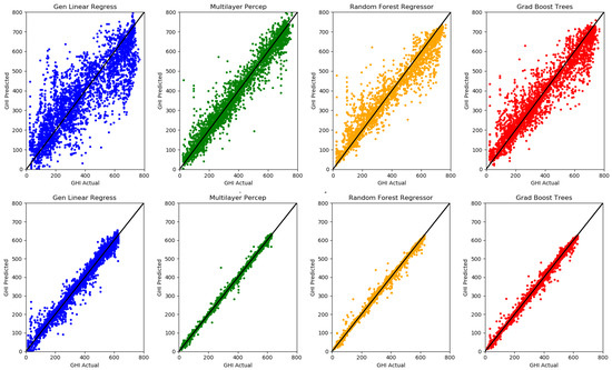
Figure 12.
Scatterplots of GHI Actual (W/m) versus GHI Predicted for the four Machine Learning Models (General Linear Regression, Multi-Layer Perceptron, Random Forest Regressor, Gradient Boosted Trees) using pixel images on: the five Moderately Cloudy Days dataset (Top Row) and the five Clear Sky Days dataset (Bottom Row).
An interesting question arises: How much additional accuracy is obtained by using the finer sampled resized images at the expense of larger data file sizes and longer runtimes? Statistical sampling and information theory would suggest that, at some point, a law of diminishing returns will occur. To answer this question, Case Study 2 involves only one day of moderately cloudy observations taken on 17 October 2015, and running the four machine learning models with resized images of , , and pixel resolutions. Table 7 and Figure 13 show the results. First note that the size of the CSV data file used as input increases dramatically: 3, 111, and 442 MB, respectively. This strongly suggests a need for other input formats for the training and test data such as ubyte encoding or raw JPEGs, and ultimately the use of CNN. Runtimes also increase for all the models with MLP the most egregious: 139, 444, and 1309 s, respectively. Accuracies do improve, but only to a certain point. In passing from to , the values go from 0.90, 0.95, 0.93, and 0.95, respectively, to 0.94, 0.99, 0.95, 0.97, respectively, but, in going to the images, they level off and, in the case of RFR, they actually get slightly worse, going from to . This is confirmed by the scatterplots of Actual GHI versus Predicted GHI displayed in Figure 13: while there is improvement in going from (not displayed) to , the graphs for the two finer resolutions are practically indistinguishable visually for all four of the machine learning models.
Table 7.
Results for 17 October 2015 with resized subimage shapes of .
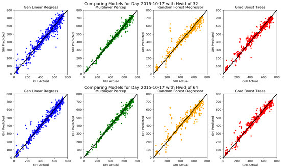
Figure 13.
Scatterplots of GHI Actual versus GHI Predicted for one day of data (17 October 2015) for the four Machine Learning Models with resized images of: pixel (Top Row); and pixel (Bottom Row). While there is improvement in passing from pixel to the pixel resized images, the latter and the pixel images are virtually indistinguishable visually.
The most important outcome of this study is the critical fact that the Pi camera on the Sky-Imager can be used as a GHI measurement instrument as well as for recording all-sky images. While it lacks the accuracy of a pyrheliometer that may cost 100 times as much as the $30 Pi Noir camera, the image sequence is already there for forecasting ramps. Why not use it to estimate GHI in real time? This information could be combined with readings from a Hardkernel Weatherboard sensor to provide a wealth of information to a micro-grid management system via MQTT or DDS protocols.
Directions for longer range research are varied. All inputs and outputs that are treated as deterministic in this study should actually be considered as stochastic: all quantities are random variables. Distinct from stochastic gradient descent used in machine learning to avoid entrapment at a local minimum, this approach recognizes that, when noise is taken into account, one is solving an evolution problem in a space of probability measures [30]. The use of various preconditioning strategies such as Sobolev inner products to smooth gradients could substantially enhance convergence. Finally, while the offline training is currently considered a one time proposition (that does depend heavily upon location and season), one can envision “continual learning” in which the networks use days and weeks of newly acquired data to “learn” how to refine the weights to achieve still better accuracies.
Author Contributions
W.R.J. provided expertise in image processing and neural networks; R.V.-A. conceived the Sky-Imager hardware and gathered the NREL data; A.M. analyzed the data; and W.R.J. and A.M. contributed to writing the paper.
Acknowledgments
This research made was possible by the partnership between the Texas Sustainable Energy Research Institute of The University of Texas at San Antonio and the San Antonio electric utility CPS Energy.
Conflicts of Interest
The authors declare no conflict of interest.
References
- Guerrero-Lemus, R.; Shephard, L. Low Carbon Energy in Africa and Latin America: Renewable Technologies, Natural Gas and Nuclear Energy (Lecture Notes in Energy), 1st ed.; Springer: Berlin, Germany, 2017. [Google Scholar]
- Richardson, W.J.; Krishnaswami, H.; Vega, R.; Cervantes, M. A low cost, edge computing, all-sky imager for cloud tracking and intra-hour irradiance forecasting. Sustainability 2017, 9, 482. [Google Scholar] [CrossRef]
- Richardson, W.; Krishnaswami, H.; Shephard, L.; Vega, R. Machine Learning versus Ray-Tracing to Forecast Irradiance for an Edge-Computing SkyImager. In Proceedings of the 2017 19th International Conference on Intelligent System Application to Power Systems (ISAP), San Antonio, TX, USA, 17–20 September 2017. [Google Scholar] [CrossRef]
- Yang, D.; Kleissl, J.; Gueymard, C.; Pedro, H.; Coimbra, C. History and trends in solar irradiance and PV power forecasting: A preliminary assessment and review using text mining. Sol. Energy 2018, 168, 60–101. [Google Scholar] [CrossRef]
- Cervantes, M.; Krishnaswami, H.; Richardson, W.; Vega, R. Utilization of Low Cost, Sky-Imaging Technology for Irradiance Forecasting of Distributed Solar Generation. In Proceedings of the 2016 IEEE Green Technologies Conference (GreenTech), Kansas City, MO, USA, 6–8 April 2016. [Google Scholar] [CrossRef]
- Cañadillas, D.; Richardson, W.J.; González-Díaz, B.; Shephard, L.; Guerrero-Lemus, R. First Results of a Low Cost All-Sky Imager for Cloud Tracking and Intra-Hour Irradiance Forecasting serving a PV-based Smart Grid in La Graciosa Island. In Proceedings of the International 2017 IEEE Photovoltaic Specialists Conference, Washington, DC, USA, 25–30 June 2017. [Google Scholar]
- Wood-Bradley, P.; Zapata, J.; Pye, J. Cloud tracking with optical flow for short-term solar forecasting. In Proceedings of the 50th Annual Australian Solar Energy Society Conference (Solar 2012), Melbourne, Australia, 6–7 December 2012. [Google Scholar]
- Lucas, B.; Kanade, T. An Iterative Image Registration Technique with an Application to Stereo Vision. In Proceedings of the 7th International Joint Conference on Artificial Intelligence (IJCAI), Vancouver, BC, Canada, 24–28 August 1981; pp. 674–679. [Google Scholar]
- Benediktsson, J.; Swain, P.; Ersoy, O. Neural Network Approaches Versus Statistical Methods in Classification of Multisource Remote Sensing Data. IEEE Trans. Geosci. Remote Sens. 1990, 28, 540–552. [Google Scholar] [CrossRef]
- Li, Q.; Lu, W.; Yang, J.; Wang, J. Thin Cloud Detection of All-Sky Images Using Markov Random Fields. IEEE Geosci. Remote Sens. Lett. 2012, 9, 417–421. [Google Scholar] [CrossRef]
- Chu, Y.; Pedro, H.; Coimbra, C. Hybrid intra-hour DNI forecasts with sky image processing enhanced by stochastic learning. Sol. Energy 2013, 98, 592–603. [Google Scholar] [CrossRef]
- Guo, W.; Xue, H. Crop Yield Forecasting Using Artificial Neural Networks: A Comparison between Spatial and Temporal Models. Math. Probl. Eng. 2014, 2014, 1–7. [Google Scholar] [CrossRef]
- Lee, H.; Piao, M.; Shin, Y. Wind Power Pattern Forecasting Based on Projected Clustering and Classification Methods. ETRI J. 2015, 37, 283–294. [Google Scholar] [CrossRef]
- Candanedo, L.; Feldheim, V.; Deramaix, D. Data driven prediction models of energy use of appliances in a low-energy house. Energy Build. 2017, 140, 81–97. [Google Scholar] [CrossRef]
- Mallat, S. Understanding deep convolutional networks. Phil. Trans. R. Soc. A 2016. [Google Scholar] [CrossRef] [PubMed]
- Salomon, R. Evolutionary Algorithms and Gradient Search: Similarities and Differences. IEEE Trans. Evol. Comput. 1998, 2, 45–55. [Google Scholar] [CrossRef]
- Cowan, J. Discussion: McCulloch-Pitts and related neural nets from 1943 to 1989. Bull. Math. Biol. 1990, 52, 73–97. [Google Scholar] [CrossRef]
- Schmidhuber, J. Deep Learning in Neural Networks: An Overview. Neural Netw. 2015, 61, 85–117. [Google Scholar] [CrossRef] [PubMed]
- Bengio, Y.; Courville, A.; Vincent, P. Representation Learning: A Review and New Perspectives. IEEE Trans. Pattern Anal. Mach. Intell. 2013, 35, 1798–1828. [Google Scholar] [CrossRef] [PubMed]
- Bengio, Y.; LeCun, Y.; Hinton, G. Deep Learning. Nature 2015, 521, 436–444. [Google Scholar]
- Liu, W.; Wang, Z.; Liu, X.; Zeng, N.; Liu, Y.; Alsaadi, F. A survey of deep neural network architectures and their applications. Neurocomputing 2017, 234, 11–26. [Google Scholar] [CrossRef]
- Raschka, S. Python Machine Learning; PACKT Publishing—Open Source: Birmingham, UK, 2016. [Google Scholar]
- Hofmann, M.; Klinkenberg, R. (Eds.) RapidMiner—Data Mining Use Cases and Business Analytics Applications, 1st ed.; Chapman and Hall/CRC: New York, NY, USA, 2013. [Google Scholar]
- Tripathi, R.; Kumari, V.; Patel, S.; Singh, Y.; Varadwaj, P. Prediction of IncRNA using Deep Learning Approach. In Proceedings of the 5th Annual International Conference on Advances in Biotechnology (BioTech), Kanpur, India, 13–15 March 2015; pp. 138–142. [Google Scholar]
- Arora, A.; Candel, A.; Lanford, J.; LeDell, E.; Parmar, V. Deep Learning with H2O.; H2O.ai, Inc.: Mountain View, CA, USA, 2016. [Google Scholar]
- Click, C.; Lanford, J.; Malohlava, M.; Parmar, V.; Roark, H. Gradient Boosted Models with H2O.; H2O.ai, Inc.: Mountain View, CA, USA, 2016. [Google Scholar]
- Pedregosa, F.; Varoquaux, G.; Gramfort, A.; Michel, V.; Thirion, B.; Grisel, O.; Blondel, M.; Prettenhofer, P.; Weiss, R.; Dubourg, V.; et al. Scikit-learn: Machine Learning in Python. J. Mach. Learn. Res. 2011, 12, 2825–2830. [Google Scholar]
- Hinton, G.; Salakhutdinov, R. Reducing the dimensionality of data with neural networks. Science 2006, 313, 504–507. [Google Scholar] [CrossRef] [PubMed]
- Reno, M.; Hansen, C.; Stein, J. Global Horizontal Irradiance Clear Sky Models: Implementation and Analysis; Sandia National Laboratories: Albuquerque, NM, USA, 2012. [Google Scholar]
- Ambrosio, L. Evolution problems in spaces of probability measures. Phys. D. Nonlinear Phenom. 2010, 239, 1446–1452. [Google Scholar] [CrossRef]
© 2018 by the authors. Licensee MDPI, Basel, Switzerland. This article is an open access article distributed under the terms and conditions of the Creative Commons Attribution (CC BY) license (http://creativecommons.org/licenses/by/4.0/).