Fast and Precise Soft-Field Electromagnetic Tomography Systems for Multiphase Flow Imaging

Ruhr-University Bochum, Institute of Electronic Circuits, Universitätsstrasse 150, 44780 Bochum, Germany
*
Author to whom correspondence should be addressed.
Energies 2018, 11(5), 1199; https://doi.org/10.3390/en11051199
Submission received: 10 April 2018
/
Revised: 30 April 2018
/
Accepted: 4 May 2018
/
Published: 9 May 2018
(This article belongs to the Special Issue Electric Fields in Energy & Process Engineering)
Abstract
:In the process industry, measurement systems are required for process development and optimization, as well as for monitoring and control. The processes often involve multiphase mixtures or flows that can be analyzed using tomography systems, which visualize the spatial material distribution within a certain measurement domain, e.g., a process pipe. In recent years, we studied the applicability of soft-field electromagnetic tomography methods for multiphase flow imaging, focusing on concepts for high-speed data acquisition and image reconstruction. Different non-intrusive electrical impedance and microwave tomography systems were developed at our institute, which are sensitive to the local contrasts of the electrical properties of the materials. These systems offer a very high measurement and image reconstruction rate of up to 1000 frames per second in conjunction with a dynamic range of up to 120 dB. This paper provides an overview of the underlying concepts and recent improvements in terms of sensor design, data acquisition and signal processing. We introduce a generalized description for modeling the electromagnetic behavior of the different sensors based on the finite element method (FEM) and for the reconstruction of the electrical property distribution using the Gauss–Newton method and Newton’s one-step error reconstructor (NOSER) algorithm. Finally, we exemplify the applicability of the systems for different measurement scenarios. They are suitable for the analysis of rapidly-changing inhomogeneous scenarios, where a relatively low spatial resolution is sufficient.
1. Introduction
In the process industry, the analysis of multiphase mixtures and flows is an important and challenging task for apparatus and process design, as well as for process monitoring and control. This is the basis for safe, efficient and economical production of, e.g., oil and gas, chemicals or pharmaceuticals. For accurate volume and mass flow measurements, as well as for apparatus and process design, the knowledge of the spatial material distribution of multiphase flows in a certain measurement domain is beneficial or even essential. Tomography systems enable one to reconstruct this distribution from which the flow regime and process parameters can be derived. Several different tomographic methods have been applied for multiphase flow analysis. These include electrical impedance, magnetic induction, microwave, ultrasound, optical, magnetic resonance, X-ray and gamma-ray tomography methods [1,2].
Hard-field electromagnetic methods—e.g., X-ray or gamma-ray tomography—are based on high-frequency electromagnetic waves, which propagate along straight lines through the material in the measurement domain independent of its distribution. In contrast, soft-field methods utilize low-frequency electromagnetic fields or waves, which strongly interact with the material. Therefore, modeling the electromagnetic behavior of the measurement domain, as well as image reconstruction are more complicated and computationally demanding. Furthermore, the achievable spatial resolution is significantly lower. However, soft-field methods are advantageous in terms of costs, instrument size and flexibility, and they avoid ionizing radiation, as well as radioactive sources. They include microwave tomography (MWT), magnetic induction tomography (MIT) and electrical impedance tomography (EIT). The latter comprises galvanically-coupled EIT and capacitively-coupled EIT. This paper focuses on the MWT and EIT methods, which enable one to determine an approximation of the cross-sectional distribution of electrical properties—electrical conductivity and permittivity—based on measurements of the electromagnetic fields at the boundary of the measurement domain. The distribution of the materials can be derived due to the contrast of their electrical properties.
EIT utilizes electric fields, whose wavelengths are significantly larger than the instrument size, and thus, the electrostatic approximation is valid. In contrast, MWT is based on the propagation of electromagnetic waves, where the wavelength is typically in the same order of magnitude as the size of the measurement domain. Thus, modeling the electromagnetic behavior is more complex. Both methods have been investigated in conjunction with medical, biomedical, as well as agricultural applications [3,4,5,6] and, furthermore, as alternative techniques for industrial process monitoring and multiphase flow imaging [7,8,9]. The application of EIT and MWT for multiphase flow analysis is a difficult task [9,10], especially in terms of instrument integration, sensitivity, measurement rate, as well as reconstruction stability and rate. In recent years, we developed concepts and systems for EIT and MWT striving to overcome the following reported challenges [9,11]:
- A non-intrusive sensor that is robust against high pressure, corrosive chemicals and large variations in temperature and that allows for efficient signal coupling, high isolation between the sensor ports, as well as accurate and computationally-efficient modeling of the electromagnetic behavior;
- Data acquisition with a high measurement rate in conjunction with a high measurement precision, accuracy and dynamic range;
- Accurate and efficient modeling of the electromagnetic behavior of the sensor for a wide range of electrical properties;
- A method for fast reconstruction of the material distribution, which is robust against stochastic and deterministic system errors.
This paper provides an overview of the underlying concepts and presents recent improvements and results. In Section 2, we introduce a generalized description for modeling the electromagnetic behavior of EIT and MWT sensors based on the finite element method (FEM) and for the reconstruction of the electrical property distribution.
To achieve fast reconstruction, we utilize Newton’s one-step error reconstructor (NOSER) algorithm, which is derived from the Gauss–Newton method. In Section 3, the sensor design concepts, as well as the data acquisition and signal processing methods are described. The applicability of the developed systems for multiphase mixture and flow analysis is investigated in Section 4. Firstly, the phase distribution is reconstructed for different static dielectric phantoms modeling multiphase mixtures. Secondly, the galvanically- and capacitively-coupled EIT systems are utilized to monitor a mixing process of water and sodium chloride (NaCl) and an oil-gas two-phase flow, respectively. In Section 5, the main results, as well as the capabilities and limitations of the modalities are discussed, and further research topics are described.
2. Imaging Method
EIT and MWT are methods for imaging of the electrical property distribution, typically in a cross-sectional plane. Multiple measurement ports—e.g., electrodes, antennas or waveguides—are arranged at the surface of the measurement domain. Based on the measurement of the port quantities, which are voltages V and currents I (EIT) or equivalent wave quantities a and b of incident and reflected waves (MWT), the distribution of the electrical properties can be reconstructed. In the case of linear materials, the port quantities are linked by the admittance matrix and the scattering matrix , respectively,
The matrices depend on the geometry of the imaging domain and the measurement ports, as well as on the distribution of the total complex-valued conductivity:
which describes the electrical properties of the materials combining the electrical conductivity and permittivity . and denote the permittivity of a vacuum and the relative permittivity of the material, respectively. In MWT, the electrical properties of the materials are often described by the total relative permittivity, which includes the electrical conductivity:
The determination of the matrices and for a specified material distribution is denoted as the forward problem. This can be solved based on accurate modeling of the electromagnetic behavior of the measurement domain (forward model), which is described in Section 2.1. The utilized method to reconstruct the material distribution based on the measured port quantities and the forward model is presented in Section 2.2. For the following explanations, we use the EIT-related notation of the electrical properties (total conductivity) and the port quantities (admittance matrix) from which the MWT-related notation can be derived.
2.1. Modeling the Electromagnetic Behavior
Assuming non-magnetic materials, the electromagnetic behavior of the imaging domain can be modeled by the following three-dimensional partial differential equation for the electrical field :
where the vector field describes the (externally) excited current density and denotes the magnetic permeability of a vacuum.
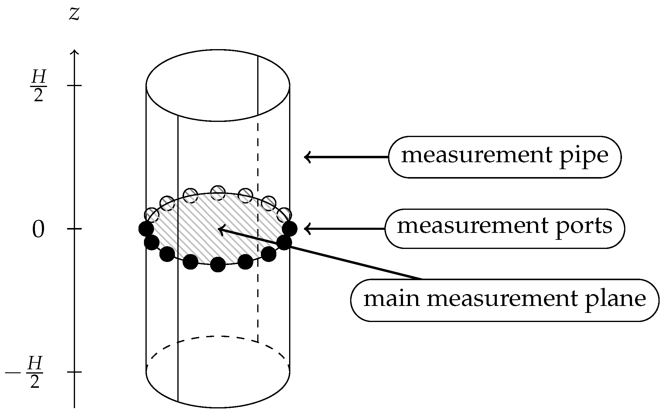
Figure 1 shows a typical measurement setup of the electromagnetic tomography for multiphase flow imaging in pipes. The measurement ports are evenly distributed along the circumference of the pipe. Assuming a uniform material distribution along the z-axis, this setup allows one to approximate the electromagnetic behavior in by a series of equations in and to reconstruct the two-dimensional distribution of the electrical properties in the main measurement plane (). The electric field can be assumed to be symmetric with the main measurement plane with a finite extension H and, thus, be described by a cosine series:
Applying Equation (6) to Equation (5) leads to:
where the series components of the excited current density are defined equivalent to .
2.1.1. Microwave Tomography
In the case of MWT, the electromagnetic behavior is usually described in terms of the wave number instead of the conductivity. Equation (7) can be rewritten as:
where the series components of the wave number are defined as:
2.1.2. Electrical Impedance Tomography
Due to the low frequency of the electrical fields used in EIT, the electrostatic approximation is valid, and the electric field can be expressed by the scalar potential field :
2.1.3. Solving the Forward Problem
In order to solve Equations (8) and (12), respectively, we utilized the finite element method (FEM). The main advantages of the FEM over other numerical methods—e.g., finite difference method (FDM) or finite volume method (FVM)—are the ease and quality of approximation of complicated (round) structures. Furthermore, the discretization leads to sparse systems of linear equations, which can be efficiently solved using GPUs. Besides parallel computing using GPUs, there are other methods to accelerate the computation process, which are based on improvements in terms of either the problem formulation or the numerical solution process as described in [12] and the references therein. However, many of them are not applicable or advantageous in the presented case due to the utilized irregular mesh and the relatively small size of the problem.
Using the FEM, a 2D model of the measurement domain (sensor) is generated by a discretization using triangular elements with piecewise constant electrical properties. The model includes the measurement domain, as well as the measurement ports and must consider the boundary conditions. Applying the FEM to Equations (8) and (12) leads to a linear system of equations for the discretized electric field and potential, respectively, which are solved iteratively using the biconjugate gradient stabilized (BiCGSTAB) method [13]. Further details are described in [14].
2.2. Image Reconstruction
The reconstruction of the spatial conductivity distribution based on the measured port quantities represents a highly non-linear and ill-posed inverse problem:
This problem can be solved using different algorithms, which can be divided into linear and non-linear algorithms. The latter includes direct methods as contrast source inversion [15] and iterative methods as Gauss–Newton [16], conjugate-gradients [17] or Landweber [18]. We utilized the Gauss–Newton method and the derived linear NOSER algorithm [19] due to its efficient implementation and improved stability. An overview of the available algorithms for soft-field tomography is given in [20].
The inverse problem can be expressed in terms of an optimization problem for the conductivity distribution:
with the error function:
is the measured admittance matrix and is calculated for a specified distribution using the forward model. Applying the Gauss–Newton method to Equation (14) leads to an iterative equation for the approximate solution of the conductivity distribution:
where the current solution is updated after each iteration. The step size is calculated based on the linearization of the error function at the solution of the previous step:
The calculation of the iterative solution is computationally demanding and time-consuming since the forward problem has to be solved for each iteration step. To achieve a sufficiently high image reconstruction rate for flow imaging, linear methods are often used to solve the inverse problem. The NOSER algorithm is a linear direct method, which is derived from the Gauss–Newton method and determines a first-order deviation from a reference distribution :
As a second step, the admittance matrix calculated using the forward model is replaced by , which represents the measured port quantities in the case of the reference distribution:
This leads to a reduction of additive systematic errors, as well as increased reconstruction stability. The algorithm offers a high performance implementation since the forward problem has to be solved only once for the reference distribution.
To improve the reconstruction stability, which is often insufficient due to the limited measurement precision and accuracy, a priori information about the material distribution has to be included. By applying the Tikhonov regularization [21] to Equation (14), the solution of the inverse problem depends on an additional constraint:
with the penalty function:
For the linear differential operator , we use a Laplacian filter, the application of which leads to a smooth spatial conductivity distribution, i.e., high spatial frequencies are suppressed depending on the regularization factor . To achieve a high image reconstruction rate of up to 1000 frames per second, the implementation is optimized for parallel computing using a graphics processing unit (GPU) as described in [14].
3. Systems
In this section, we describe the sensor and data acquisition concepts of the three soft-field tomography systems—galvanically-coupled EIT, capacitively-coupled EIT and MWT—which were developed to overcome the challenges related to real-time multiphase flow imaging. Designing soft-field tomography systems, it has to be taken into account that the reconstruction accuracy and stability depend on the number of independent measurements, as well as on the measurement precision and accuracy. On the one hand, an increased number of ports leads to an increased number of possible independent measurements and, thus, a potentially higher spatial resolution and reconstruction stability. On the other hand, it results in an increased complexity of the system and a decreased measurement rate. Furthermore, the measurement precision can decrease due to a reduced sensor sensitivity, which is related to the size of the ports.
3.1. EIT
The EIT is used to determine the spatial distribution of the complex-valued conductivity inside a given measurement domain. Electrodes are placed at discrete positions along the circumference of the imaging domain. The complex-valued conductivity distribution can be calculated from measured voltages and currents at all electrodes.
Two main aspects of an EIT system for process visualization are the measurement rate and the dynamic range. To achieve good reconstruction results, a high dynamic range and minimization of the noise level are required, because geometrically small inhomogeneities have a low impact on the measured signals, due to the large wavelengths of the excitation signals in relation to the geometric dimensions of the environment. Additionally the measurement signals at electrodes with a large distance from the excitation electrodes are very small, and thus, the measurements are strongly affected by electronic noise. Brown and Seagar [22] found that the voltages between adjacent electrodes are typically within a dynamic range of 32 dB. Accordingly, a measurement dynamic range greater than 92 dB is required to resolve variations of 0.1% of the electrical conductivity. Furthermore, a large measurement rate is required to assure that no significant changes of the conductivity distribution occur during a single measurement. In common EIT systems, the excitation of different electrodes and the associated voltage or current measurements at all other electrodes are performed sequentially using a time-division multiplexing (TDM) procedure. To increase the measurement rate, the measurement time has to be decreased. Consequently, the dynamic range of these systems is decreased.
To realize a high measurement rate in combination with a high dynamic range, we adapted the frequency-division multiplexing (FDM) technique for EIT [23]. Multiple excitation signals with orthogonal frequencies are used at different electrodes at the same time. The superimposed measurement signals can be separated and assigned to the different excitation signals. In this way, the measurement rate can be increased without decreasing the measurement time. Therefore, a data acquisition unit (DAU) is required, which allows for parallel excitation and measurement.
We developed a galvanically- and a capacitively-coupled EIT system with a parallel hardware architecture intended for real-time analysis of multiphase mixtures and flows. The sensor design and modeling, as well as the data acquisition and signal processing will be explained for both systems in the following subsections.
3.1.1. Sensor and Modeling
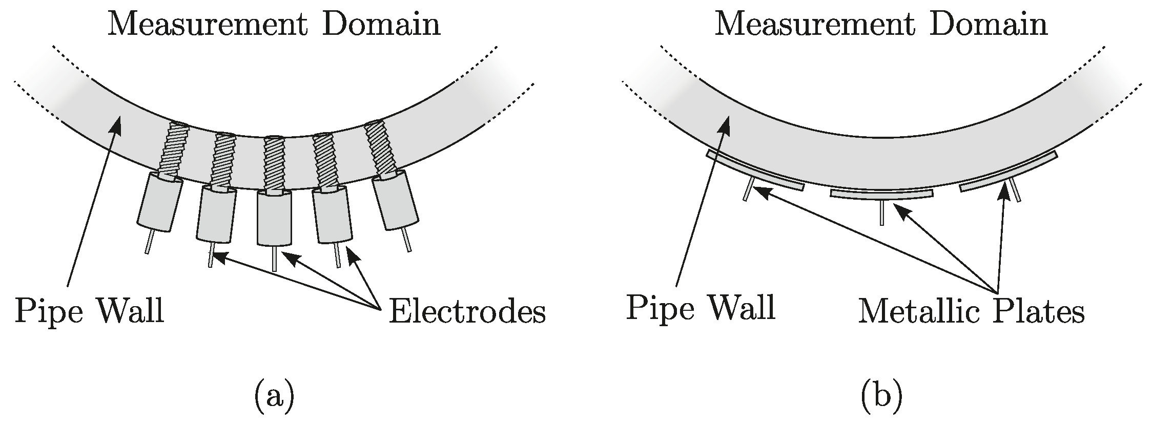
For the EIT, there are generally two different methods for coupling and decoupling electrical signals to and from the measurement domain: galvanic and capacitive coupling. In the case of the former method, an electrode ring with equidistant electrodes is mounted at the circumference of the domain. Each electrode is screwed through a non-conductive wall; thus, the end faces of the electrodes are flush with the wall, and an electrically-conductive connection between the electrodes and the measurement domain is realized. For the capacitive coupling, metallic plates are circularly distributed on the outer surface of a non-conductive pipe. Electric fields with a sufficiently high frequency are coupled through the wall into the measurement domain. Horizontal cross-sections of both coupling variants are shown in Figure 2.
Each variant has certain advantages and drawbacks and is suitable for different measurement scenarios. The electrodes of the galvanically-coupled sensor are usually significantly smaller compared to the metallic plates of the capacitively-coupled sensor, and thus, more electrodes can be mounted around the measurement domain. This leads to an increased spatial resolution and reconstruction stability. However, galvanically-coupled systems are only suitable for conductive background materials, and the electrodes are susceptible to contamination or abrasion due to the direct contact with the materials. The capacitive coupling method is more robust, since the metallic plates are separated from the measurement domain, and suitable for non-conductive materials.
The developed galvanically-coupled sensor [24] consists of a polymethyl methacrylate (PMMA) pipe, with an inner diameter of and a height of , and an electrode ring with 36 gold-plated electrodes, which is mounted at the circumference. Eighteen electrodes are used for current excitation and the other 18 electrodes are for voltage measurement. Each electrode has a diameter of .
The capacitively-coupled sensor consists of a zirconium dioxide ceramic pipe, with an inner diameter of and a height of 400 mm, and 16 metallic plates, which are 9 mm wide and 100 mm high. The ceramic pipe has a large relative permittivity of 28, which allows for effective signal coupling through the wall. Additionally, it is resistant to abrasive fluids, almost all acids, high pressures (up to 2000 MPa) and high temperatures (up to 900 in air). To minimize stray capacitances, a second layer of metallic plates is mounted on the first layer, separated by an acrylic glass pipe with a wall thickness of 3 mm. These electrodes are used in a driven shield configuration [25].
The electromagnetic behavior of both sensors is described by Equations (6) and (11). The effective height used in these equations is chosen as 300 mm and 100 mm for the galvanically- and capacitively-coupled sensor, respectively. The number of used series components n was determined based on a comparison of simulation and measurement results. For the galvanically-coupled sensor, it has been shown that for , the relative root mean square (RMS) error reached a constant minimum [14]. For the capacitively-coupled sensor, was determined.
3.1.2. Data Acquisition and Signal Processing
Both EIT systems comprise parallel excitation, measurement and signal processing units in order to be able to apply the FDM measurement procedure. Thereby, the systems achieve measurement rates with up to 1000 complete measurement cycles per second in combination with a measurement dynamic range of .
In Figure 3, a simplified block diagram of the developed galvanically-coupled system is shown. The system consists of the sensor, nine parallel excitation sources, 18 parallel voltage measurement channels and a digital system control unit, as well as a personal computer (PC) with a GPU for fast image reconstruction. The time-harmonic carrier signals in the frequency range of 200 to 300 kHz are generated by using direct digital synthesizers (DDS). Controlled floating current sources have been realized to ensure constant excitation amplitudes independent of the changing load impedance. The parallel measurement unit is based on 18 synchronously sampled analog-to-digital converters (ADC) with an amplitude resolution of 24 bit and a spurious free dynamic range of 120 dB. Each ADC digitizes the preamplified differential voltage signal between two electrodes. The digital signal processing (DSP) is performed on field programmable gate arrays (FPGA).
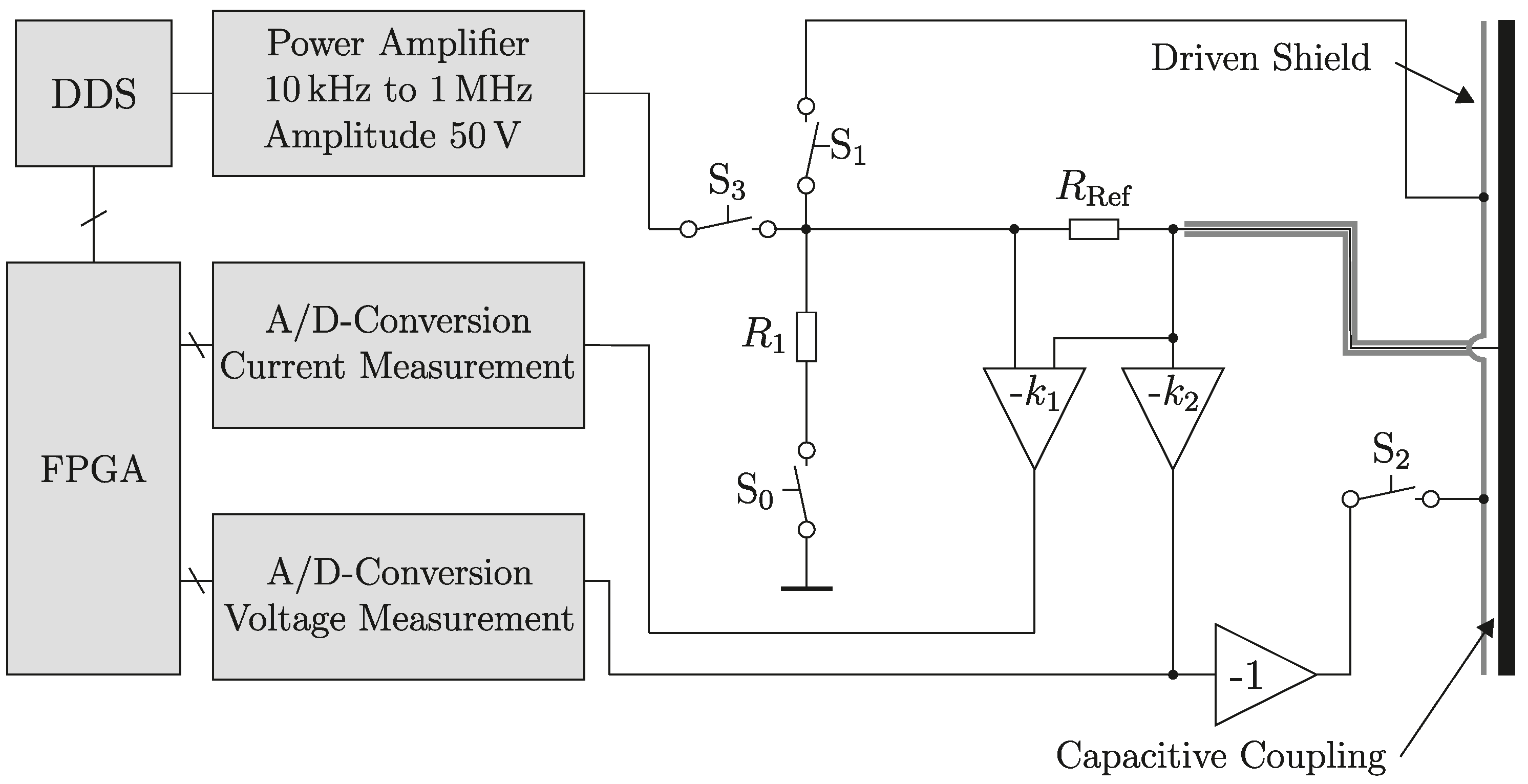
In contrast to the galvanically-coupled system, the excitation and measurement ports are not separated in the case of the capacitively-coupled system. Here, 16 identical signal processing units are used for all 16 measurement ports. A block diagram of one signal processing unit is shown in Figure 4. Each channel can be used in excitation or receive mode. In excitation mode, time-harmonic carrier signals in the frequency range of 450 to 550 kHz are generated using a DDS. The carrier signal is amplified to an amplitude of 50 V to compensate the attenuation of the pipe wall and thus to maximize the signal strength at the receive channels. In receive mode, the excitation signal is switched off, and the signal path is terminated by the resistance . The port current and voltage are measured by two ADC. An FPGA controls the DDS and performs the parallel DSP.
3.2. MWT
Microwave tomography is an imaging method reconstructing the distribution of the complex-valued relative permittivity based on measurements of the scattered electromagnetic fields at the boundary of the imaging domain. Although the utilized method determines the distribution-based single-frequency measurement data, a large frequency range of the sensor and the DAU is beneficial due to the following reasons. The selection of the reconstruction frequency can be adapted to the measurement scenario. In the case of low-contrast materials or small changes in the material distribution, the scattering parameters change only slightly compared to the reference scenario. Measurement data at high frequencies should be utilized for reconstruction since the sensitivity of the sensor often increases with increasing frequency. This leads to an improved signal-to-noise ratio assuming a limited, but frequency independent measurement precision. In the case of a large change in the material distribution or high-contrast materials, the reconstruction frequency should be significantly reduced to limit the deviation of scattering parameters and maintain reconstruction stability [26]. Furthermore, the reconstruction results can be improved by using measurement data at multiple frequencies as shown in [26].
The upper frequency limit is determined by the following issues. Firstly, the attenuation of microwaves in conductive materials, i.e., salt water, increases with increasing frequency. Secondly, the complexity of the forward model and the computational effort increase while the achievable accuracy decreases due to multimode wave propagation and a necessary reduction of the mesh element size at high frequencies. The lower frequency limit depends on the maximum acceptable size of the measurement ports and, thus, the minimum number of ports. The complexity of the data acquisition unit and system calibration increases with increasing bandwidth. The maximum system bandwidth is limited by the bandwidth of the measurement ports. The sensor design and the derived forward model, as well as the DAU are presented in the following subsections.
3.2.1. Sensor and Modeling
The application of MWT for multiphase flow imaging requires a special sensor design, which addresses the challenges related to multiphase flow analysis described in Section 1. Since most published MWT sensor concepts [5] are not suitable for measurements in metal or ceramic pipes, we developed a new MWT sensor concept [27].
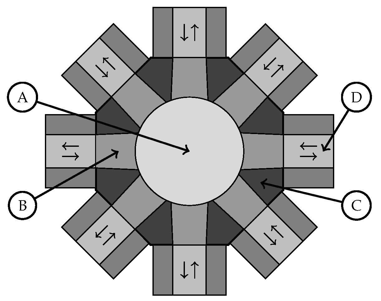
The sensor consists of a metal pipe, with an inner diameter of and a height of , and wedge-shaped dielectric windows, which are made out of a technical plastic (PEEK). The microwaves are guided from the excitation port through a rectangular waveguide and a dielectric window into the measurement domain as depicted in Figure 5. The sensor is fed from coaxial lines using rectangular waveguides with a broadband transition [28]. The selection of the frequency range is a trade-off between microwave attenuation, geometrical dimensions of the sensor, the number of sensor ports and the complexity of the data acquisition unit. We realized an eight-port sensor that is usable in the frequency range 0.7 to . The width of the dielectric windows in the z-direction is .
The electromagnetic field distribution inside the waveguides and the dielectric windows is a superposition of the multiple waveguide modes. Due to the symmetry of the waveguides, only odd transverse electric modes are excited and propagable, and the corresponding electric fields have a maximum at the main measurement plane. Furthermore, it can be assumed that the fundamental mode () is the dominating wave mode inside the windows and the measurement domain.
The forward model includes the measurement domain, the dielectric windows and the metal frame of the sensor, as well as the wave ports for excitation and measurement, which are located at the interfaces between the dielectric windows and the rectangular waveguides. The electric fields at these interfaces can be calculated from the measured scattering parameters [27]. The electromagnetic behavior can be calculated using Equations (6), (8) and (9), where and the height H depends on the position in the measurement plane. Inside the dielectric windows, the height is exactly known and equals the width of the windows (). Inside the measurement domain, the electromagnetic behavior can be accurately modeled using an effective height of .
3.2.2. Data Acquisition and Signal Processing
The input parameters of the image reconstruction algorithm are derived from the measured scattering parameters. To achieve a sufficiently high measurement rate in combination with a high dynamic range and a high measurement bandwidth at reasonable costs, a parallel-detecting custom-design data acquisition unit (DAU) is required, because commercial vector network analyzers are expensive and bulky. Most reported MWT systems utilize commercial or custom-designed DAUs based on the continuous wave (CW) network analysis method and the heterodyne principle [29]. These systems offer a high measurement precision and dynamic range, but the system error reduction of multiport MWT systems is complicated and the achievable measurement rate low in the case of a high number of required frequency samples. To overcome these drawbacks, we examined the applicability of the frequency-modulated continuous waves (FMCW) network analysis technique [30] for multiport MWT systems [31], which offers robust and computationally inexpensive system error reduction, resulting in an improved imaging accuracy and reconstruction stability.
We recently designed an eight-port parallel-detecting FMCW DAU using the heterodyne principle, which allows for a higher flexibility in terms of measurement setup and parameters compared to our previously-developed homodyne prototype system presented in [31]. A block diagram of the MWT system including the DAU and a photograph of the eight-port sensor are shown in Figure 6.
The synthesizer is one of the key components of the system, and its implementation is similar to that presented in [32]. It generates two signals and , whose frequencies are linearly varied from the start to the stop frequency, e.g., 0.7 to , and differ by a small offset, e.g., . The signal is guided through an eight-port switch and a coupler to the current excitation port of the MWT sensor. The incident and reflected waves are coupled towards an eight-port receiver, where they are mixed down with the signals into the intermediate frequency (IF) range () and measured simultaneously. Each measurement port includes two measurement channels. To obtain the full scattering matrix, one measurement cycle includes eight steps during which the excitation port is varied. The DSP is performed on four FPGA, which allow for a parallelized computation of the wave quantities from which the scattering parameters are derived. A PC including a GPU is used for the reconstruction of the permittivity distribution. The developed DAU allows for broadband measurements in the entire frequency range of interest. In the case of a data acquisition time of for a single excitation, which corresponds to a theoretical measurement rate of 125 cycles per second (neglecting the DSP time), and a bandwidth of , the developed DAU offers a relative measurement uncertainty and a dynamic range of approximately and , respectively. This significantly exceeds the performance of previously-published FMCW DAUs [33,34]. All imaging examples presented in Section 4 are based on measurement data using a two-port prototype of the heterodyne DAU in conjunction with a switching matrix.
4. Imaging Results
In this section, we examine the applicability of the developed systems for multiphase flow imaging, reconstructing the material distribution in the case of static phantoms (MWT), a mixing process (galvanically-coupled EIT) and a two-phase flow (capacitively-coupled EIT), respectively. For image reconstruction, we utilized the NOSER algorithm resulting in a first-order deviation of the electrical property distribution from a reference scenario. The electrical properties of the reference material are shown in green, whereas positive and negative contrasts are indicated in red and blue, respectively. All images are scaled to the maximum absolute deviation from the reference value.
4.1. Static Multiphase Mixture
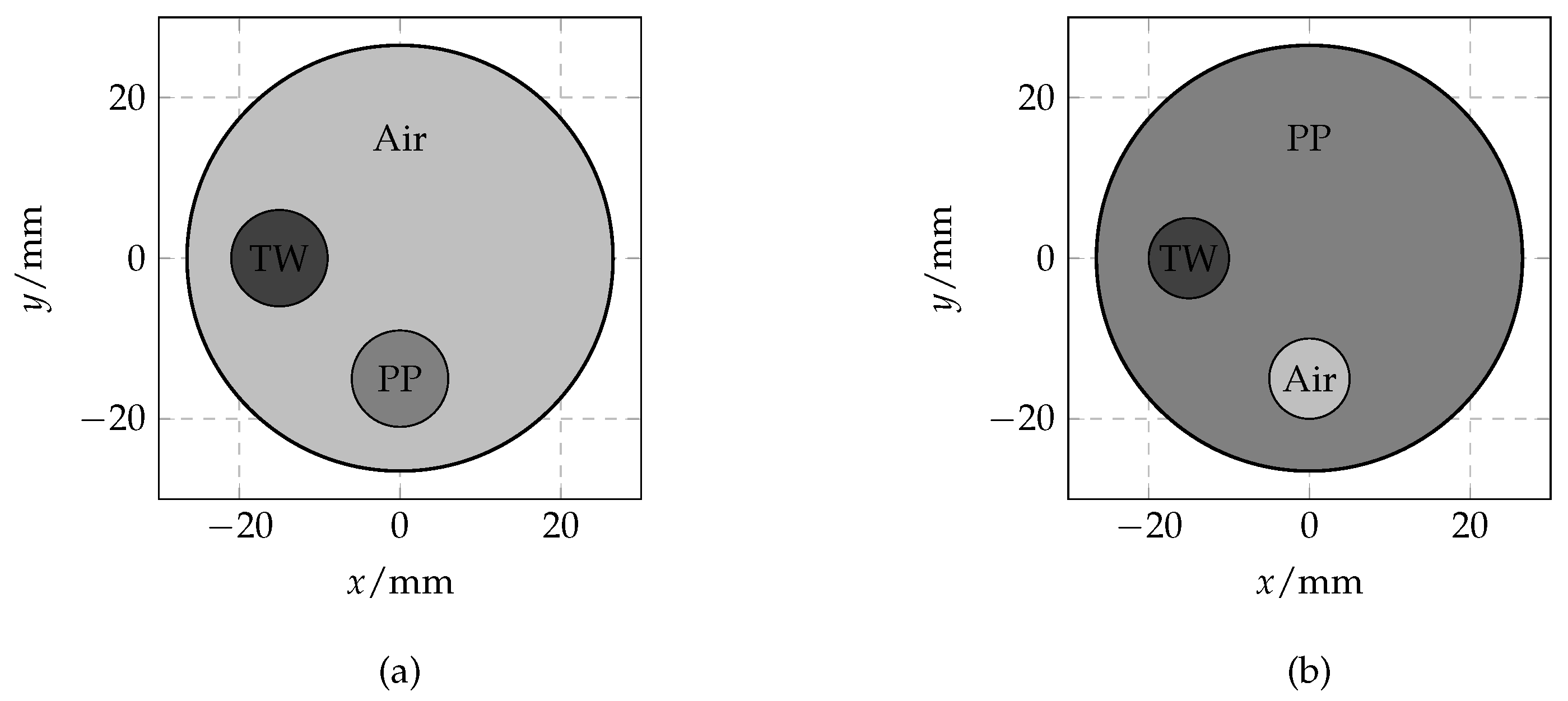
One possible application of the capacitively-coupled EIT and MWT systems is oil-gas-water flow imaging, e.g., for flow regime identification. In a first step, we tested our systems with different static phantoms, which have similar electrical properties. As materials for these phantoms, we utilized air, polypropylene (PP) and tap water (TW) with relative permittivities of , and , respectively.
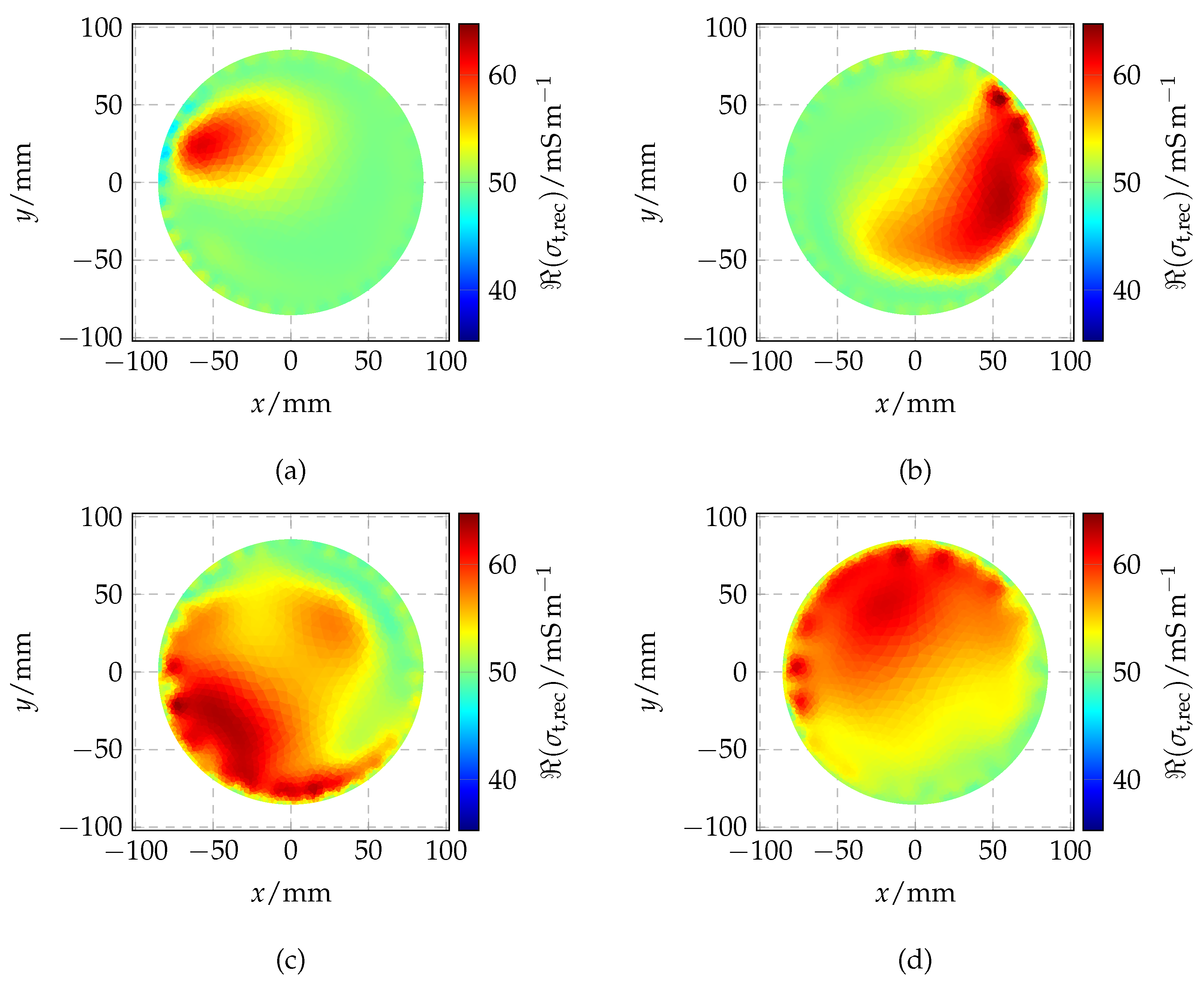
Figure 7 shows the actual material distribution for two static mixtures modeling oil/water-in-gas and gas/water-in-oil scenarios, respectively. The corresponding real part of the reconstructed permittivity distribution is shown in Figure 8. The linearization of the problem leads to a qualitative approximation of the electrical property distribution with a smooth transition from the maximum to the reference permittivity. The utilized regularization method results in a suppression of high spatial frequencies as described in Section 2.2. However, in both scenarios, the positions of the objects are accurately reconstructed, and the materials can be clearly identified due to their electrical properties, which indicates the applicability of the system for imaging of oil-gas-water mixtures. Experiments using the capacitively-coupled EIT system led to similar imaging results. The reconstruction of multiphase flows is described in Section 4.3.
4.2. Mixing Process
In this section, a visualization of a simple mixing process using the galvanically-coupled EIT system is presented. During this experiment, 2 g of sodium chloride were mixed into 13 L of tap water. The sodium chloride was poured into a concentrated spot in the measurement domain filled with tap water. The mixture was stirred in a clockwise direction by a rotating magnetic stirrer. Figure 9 shows a series of four reconstructed conductivity distributions based on measurements with a time offset of 2 s. An increase in conductivity based on the dissolving process of the sodium chloride and the movement of the mixture can be clearly observed.
4.3. Two-Phase Flow
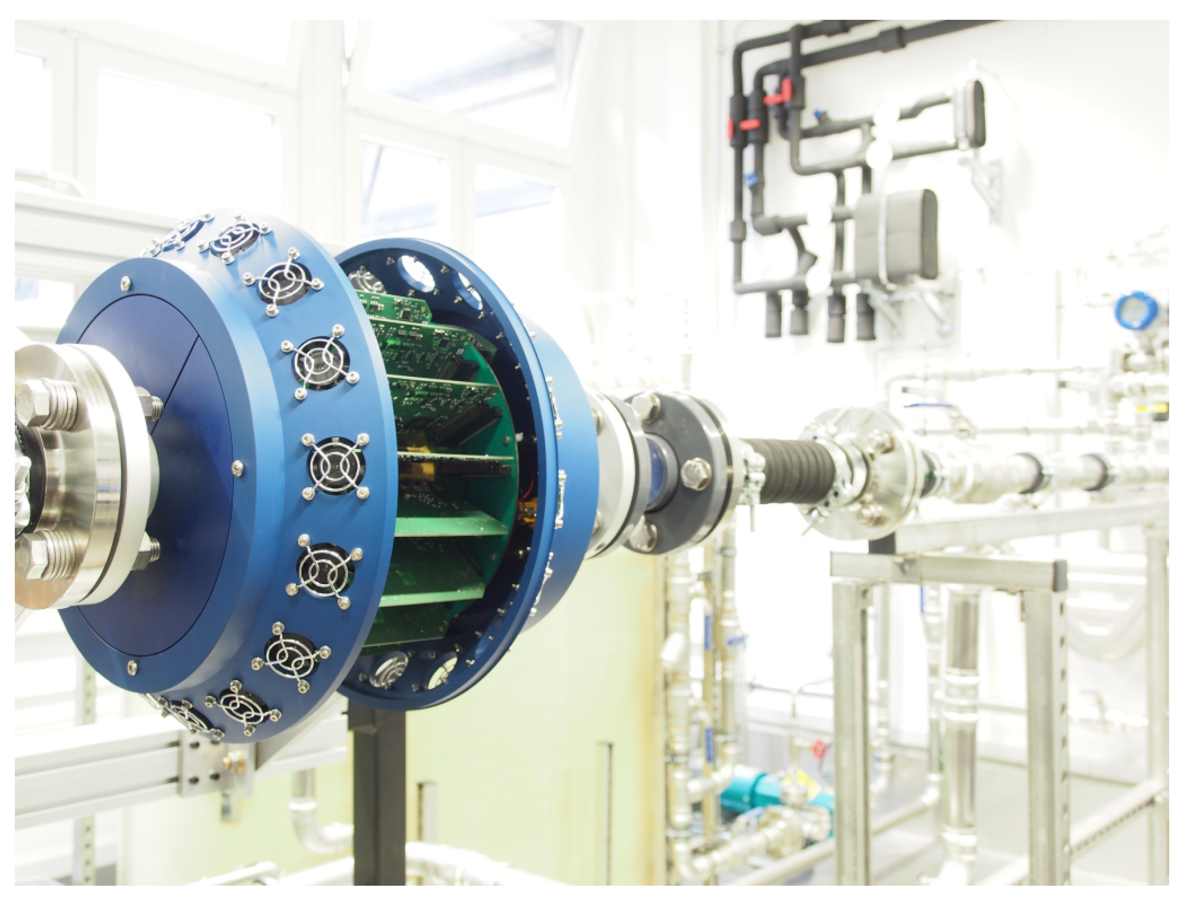
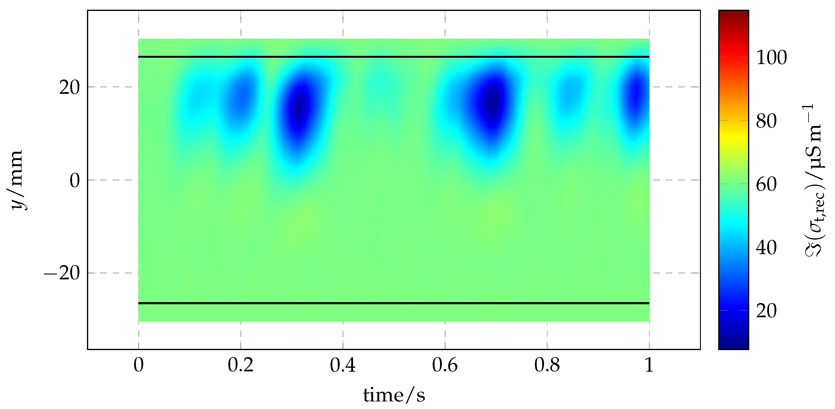
For the evaluation of the capacitively-coupled EIT system, we installed it in our multiphase flow loop, as depicted in Figure 10, and studied different intermittent two-phase flows. As one example, the system was used to analyze the transient behavior of an oil-gas slug flow. A vertical cut () of the imaginary part of the reconstructed conductivity distribution as a function of time is presented in Figure 11. The amount of gas bubbles, as well as their size, length and position along the vertical cut can be evaluated based on this measurement series.
5. Discussion and Conclusions
In this paper, we presented an overview of three different soft-field electromagnetic tomography systems—a galvanically- and a capacitively-coupled EIT, as well as an MWT system—intended for real-time imaging of multiphase mixtures and flows. The developed systems offer an as of yet unachieved combination of measurement precision, accuracy and dynamic range, as well as a measurement and image reconstruction rate of up to 1000 frames per second.
The selection of the appropriate soft-field tomography modality for the analysis of a certain process depends on the requirements of the application in terms of process integration, electrical properties of the materials involved and costs. The spatial resolution is similar for each modality, depends on the number of measurement ports and is in the order of one tenthof the pipe diameter. MWT systems can be used for conductive and non-conductive materials, and their sensitivity range can be adapted by the selection of the measurement frequency. Furthermore, FMCW-based systems offer robust system error reduction. However, compared to EIT systems, the complexity of the data acquisition unit is significantly higher, and modeling the electromagnetic behavior is more complex. Galvanically-coupled EIT systems are suitable for applications where direct contact between the measurement ports and the materials is acceptable and the background material has a sufficiently high electrical conductivity. Compared to capacitively-coupled EIT and MWT systems, the ports are significantly smaller, which results in a lower instrumentation size. Furthermore, the number of ports can be higher, which potentially leads to an increased spatial resolution. In contrast, capacitively-coupled EIT systems are suitable for applications involving conductive and non-conductive materials, as well as in the case of chemically-aggressive or abrasive materials.
In our opinion, the presented systems are beneficial tools for the analysis and optimization of processes with rapidly-changing inhomogeneous material distributions, where a relatively low spatial resolution—compared to hard-field tomography modalities—is acceptable. In current and further research, we investigate sensor, modeling and data acquisition concepts to increase the flexibility of the systems and thus simplify the integration into the process. This will allow examining the suitability for an extended range of applications. Furthermore, we study methods to derive process parameters from the reconstructed distribution of the electrical properties. Finally, a combination of two modalities may improve the achievable reconstruction quality, which will be investigated in future work.
Author Contributions
M.G. and M.M. designed the EIT systems and MWT system, respectively, and performed the corresponding experiments, as well as analyzed the data. P.G. developed and implemented the concepts for reconstruction of the electrical property distribution for the EIT and MWT systems. T.M. contributed ideas for the system concepts, the design of the components, the interpretation of results and the focus of the research activities. M.M. and M.G. wrote the paper.
Acknowledgments
The authors wish to express their gratitude to the German Federal Ministry of Economic Affairs and Energy (BMWi) and Project Management Jülich (PTJ) for funding the joint project ‘ECUP 3000—Enhanced Control of Underwater Production up to 3000 m Water Depth’ (FKZ 03SX312).
Conflicts of Interest
The authors declare no conflict of interest. The founding sponsors had no role in the design of the study; in the collection, analyses or interpretation of data; in the writing of the manuscript; nor in the decision to publish the results.
References
- Wang, M. Industrial Tomography, 1st ed.; Woodhead Publishing: Cambridge, UK, 2015; pp. 1–302. ISBN 978-1-78242-118-4. [Google Scholar]
- Thorn, R.; Johansen, A.; Hjertaker, B. Three-phase flow measurement in the petroleum industry. Meas. Sci. Technol. 2013, 24, 012003. [Google Scholar] [CrossRef]
- Holder, D. Electrical Impedance Tomography—Methods, History and Applications, 1st ed.; Institute of Physics Publishing: Bristol, UK, 2005; ISBN 978-0750309523. [Google Scholar]
- Noghanian, S.; Sabouni, A.; Desell, T.; Ashtari, A. Introduction to Microwave Imaging. In Microwave Tomography, 1st ed.; Springer: New York, NY, USA, 2014; pp. 1–20. ISBN 978-1-4939-0751-9. [Google Scholar]
- Rahiman, M.; Kiat, T.; Jack, S.; Rahim, R. Microwave Tomography Application and Approaches—A Review. J. Teknol. 2015, 73, 133–138. [Google Scholar] [CrossRef]
- Chandra, R.; Zhou, H.; Balasingham, I.; Narayanan, R.M. On the opportunities and challenges in microwave medical sensing and imaging. IEEE Trans. Biomed. Eng. 2015, 62, 1667–1682. [Google Scholar] [CrossRef] [PubMed]
- Tapp, H.; Peyton, A.; Kemsley, E.; Wilson, R. Chemical engineering applications of electrical process tomography. Sens. Actuators B Chem. 2003, 92, 17–24. [Google Scholar] [CrossRef]
- Wu, Z.; McCann, H.; Davis, L.; Hu, J.; Fontes, A.; Xie, C. Microwave-tomographic system for oil-and gas-multiphase-flow imaging. Meas. Sci. Technol. 2009, 20, 104026. [Google Scholar] [CrossRef]
- Wu, Z. Developing a microwave tomographic system for multiphase flow imaging: Advances and challenges. Trans. Inst. Meas. Cont. 2014, 37, 760–768. [Google Scholar] [CrossRef]
- Ismail, I.; Gamio, J.C.; Bukhari, S.F.A.; Yang, W.Q. Tomography for Multi-Phase Flow Measurement in the Oil Industry. Flow Meas. Instr. 2005, 16, 145–155. [Google Scholar] [CrossRef]
- Wei, K.; Qiu, C.; Primrose, K. Super-sensing technology: Industrial applications and future challenges of electrical tomography. Philos. Trans. Math. Phys. Eng. Sci. 2016, 374, 20150328. [Google Scholar] [CrossRef] [PubMed]
- Lu, M.; Peyton, A.; Wuliang, Y. Acceleration of Frequency Sweeping in Eddy-Current Computation. IEEE Trans. Magn. 2017, 53, 1–8. [Google Scholar] [CrossRef]
- Van der Vorst, H.A. A Fast and Smoothly Converging Variant of Bi-CG for the Solution of Nonsymmetric Linear Systems. SIAM J. Sci. Stat. Comput. 1992, 13, 631–644. [Google Scholar] [CrossRef]
- Gebhardt, P.; Gevers, M.; Musch, T. GPU Accelerated 2.5D Solver for Fast and Accurate Modeling of EIT Forward Problem in Tube Geometries. In Proceedings of the 7th World Congress on Industrial Process Tomography, Krakow, Poland, 2–5 September 2013; pp. 355–364. [Google Scholar]
- Van den Berg, P.M.; Kleinman, R.E. A Contrast Source Inversion Method. Inverse Probl. 1997, 13, 1607–1620. [Google Scholar] [CrossRef]
- Vauhkonen, P.J.; Vauhkonen, M.; Savolainen, T.; Kaipio, J.P. Three-dimensional electrical impedance tomography based on the complete electrode model. IEEE Trans. Biomed. Eng. 1999, 46, 1150–1160. [Google Scholar] [CrossRef] [PubMed]
- Wang, M. Inverse solutions for electrical impedance tomography based on conjugate gradients methods. Meas. Sci. Technol. 2002, 13, 101–117. [Google Scholar] [CrossRef]
- Zhang, L. Image reconstruction algorithm for electrical impedance tomography using updated sensitivity matrix. In Proceedings of the International Conference of Soft Computing and Pattern Recognition, Dalian, China, 14–16 October 2011; pp. 248–252. [Google Scholar]
- Cheney, M.; Isaacson, D.; Newell, J.C.; Simske, S.; Goble, J. NOSER: An algorithm for solving the inverse conductivity problem. Int. J. Imaging Syst. Technol. 1990, 2, 66–75. [Google Scholar] [CrossRef]
- Polydorides, N. Image Reconstruction Algorithms for Soft-Field Tomography. Ph.D. Thesis, University of Manchester, Manchester, UK, 2002. [Google Scholar]
- Vauhkonen, M.; Vadasz, D.; Karjalainen, A.; Somersalo, E.; Kaipio, J.P. Tikhonov regularization and prior information in electrical impedance tomography. IEEE Trans. Med. Imaging 1998, 17, 285–293. [Google Scholar] [CrossRef] [PubMed]
- Brown, B.; Seagar, A. The Sheffield data collection system. Clin. Phys. Physiol. Meas. 1987, 8, 91–97. [Google Scholar] [CrossRef] [PubMed]
- Gevers, M.; Gebhardt, P.; Biesenbach, B.; Vogt, M.; Musch, T. A fast electrical impedance tomography system with parallel multi-carrier excitation. In Proceedings of the 7th World Congress on Industrial Process Tomography, Krakow, Poland, 2–5 September 2013; pp. 193–202. [Google Scholar]
- Gevers, M.; Gebhardt, P.; Westerdick, S.; Vogt, M.; Musch, T. Fast electrical impedance tomography based on code-division-multiplexing using orthogonal codes. IEEE Trans. Instr. Meas. 2015, 64, 1188–1195. [Google Scholar] [CrossRef]
- Gevers, M.; Gebhardt, P.; Vogt, M.; Musch, T. An electrical capacitance tomography system allowing for complex N-Port Calibration. In Proceedings of the 7th International Symposium on Process Tomography, Dresden, Germany, 1–3 September 2015. [Google Scholar]
- Chew, W.C.; Lin, J.H. A frequency-hopping approach for microwave imaging of large inhomogeneous bodies. IEEE Mircow. Guided Wave Lett. 1995, 5, 439–441. [Google Scholar] [CrossRef]
- Mallach, M.; Gebhardt, P.; Musch, T. 2D microwave tomography system for imaging of multiphase flows in metal pipes. Flow Meas. Instr. 2017, 28, 1–14. [Google Scholar] [CrossRef]
- Mallach, M.; Musch, T. Broadband coaxial line to rectangular waveguide transition for a microwave tomography sensor. In Proceedings of the 11th European Conference on Antennas and Propagation, Paris, France, 19–24 March 2017; pp. 465–468. [Google Scholar]
- Hiebel, M. Design of a heterodyne N-port network analyzer. In Fundamentals of Vector Network Analysis, 4th ed.; Rohde & Schwarz GmbH & Co.: Munich, Germany, 2008; pp. 22–79. ISBN 978-3939837060. [Google Scholar]
- Brunfeldt, D.R.; Mukherjee, S. A novel technique for vector network measurement. In Proceedings of the 37th ARFTG Conference Digest, Boston, MA, USA, 13–14 June 1991; pp. 35–42. [Google Scholar]
- Mallach, M.; Musch, T. Fast and precise data acquisition for broadband microwave tomography systems. Meas. Sci. Technol. 2017, 28, 094003. [Google Scholar] [CrossRef]
- Mallach, M.; Storch, R.; Grys, D.-B.; Musch, T. A broadband frequency ramp generator for very fast network analysis based on a fractional-N phase locked loop. In Proceedings of the 46th European Microwave Conference, London, UK, 3–7 October 2016; pp. 1023–1026. [Google Scholar]
- Musch, T.; Schulte, B.; Schiek, B. A fast heterodyne network analyzer based on precision linear frequency ramps. In Proceedings of the 31st European Microwave Conference, London, UK, 24–26 September 2001. [Google Scholar]
- Schulte, B.; Musch, T.; Schiek, B. A fast network analyzer for the frequency range of 10 MHz to 4 GHz. In Proceedings of the 33rd European Microwave Conference, Munich, Germany, 7–9 October 2003; pp. 97–100. [Google Scholar]
Figure 1.
Schematic view of a typical measurement setup for multiphase flow imaging in a pipe with circularly-arranged measurement ports.
Figure 1.
Schematic view of a typical measurement setup for multiphase flow imaging in a pipe with circularly-arranged measurement ports.

Figure 2.
Cross-section of different coupling variants: (a) galvanic coupling; (b) capacitive coupling.
Figure 2.
Cross-section of different coupling variants: (a) galvanic coupling; (b) capacitive coupling.

Figure 3.
Simplified block diagram of the developed fast galvanically-coupled electrical impedance tomography (EIT) system. DDS, direct digital synthesizer.
Figure 3.
Simplified block diagram of the developed fast galvanically-coupled electrical impedance tomography (EIT) system. DDS, direct digital synthesizer.

Figure 4.
Block diagram of one signal processing unit of the capacitively-coupled EIT system.

Figure 5.
Schematic view of the main measurement plane of the microwave tomography (MWT) sensor: measurement domain (A), metal pipe wall (B), dielectric window (C) and rectangular waveguide (D).
Figure 5.
Schematic view of the main measurement plane of the microwave tomography (MWT) sensor: measurement domain (A), metal pipe wall (B), dielectric window (C) and rectangular waveguide (D).

Figure 6.
Block diagram of the MWT system including the data acquisition unit (DAU) and a photograph of the eight-port sensor. FMCW, frequency-modulated continuous wave.
Figure 6.
Block diagram of the MWT system including the data acquisition unit (DAU) and a photograph of the eight-port sensor. FMCW, frequency-modulated continuous wave.

Figure 7.
Measurement scenarios: (a) one tap water (TW)-filled polymethyl methacrylate (PMMA) tube and one polypropylene (PP) rod in an air-filled pipe; and (b) a PP cylinder with one TW-filled drill hole and one air-filled drill hole.
Figure 7.
Measurement scenarios: (a) one tap water (TW)-filled polymethyl methacrylate (PMMA) tube and one polypropylene (PP) rod in an air-filled pipe; and (b) a PP cylinder with one TW-filled drill hole and one air-filled drill hole.

Figure 8.
Real part of the reconstructed permittivity distribution using the MWT system: (a) first measurement scenario at GHz; and (b) second measurement scenario at GHz. The actual shape and position of the objects are indicated by the dashed circles.
Figure 8.
Real part of the reconstructed permittivity distribution using the MWT system: (a) first measurement scenario at GHz; and (b) second measurement scenario at GHz. The actual shape and position of the objects are indicated by the dashed circles.

Figure 9.
Reconstructed conductivity distribution (galvanically-coupled EIT) at different times t, visualizing the mixing process of tap water and sodium chloride (NaCl): (a) t = 0 s, (b) t = 2 s, (c) t = 4 s, and (d) t = 6 s.
Figure 9.
Reconstructed conductivity distribution (galvanically-coupled EIT) at different times t, visualizing the mixing process of tap water and sodium chloride (NaCl): (a) t = 0 s, (b) t = 2 s, (c) t = 4 s, and (d) t = 6 s.

Figure 10.
Photograph of the capacitively-coupled EIT system installed in our multiphase flow loop.

Figure 11.
Vertical cut () of the imaginary part of the reconstructed conductivity distribution (capacitively-coupled EIT) as a function of time, visualizing an oil-gas slug flow.
Figure 11.
Vertical cut () of the imaginary part of the reconstructed conductivity distribution (capacitively-coupled EIT) as a function of time, visualizing an oil-gas slug flow.

© 2018 by the authors. Licensee MDPI, Basel, Switzerland. This article is an open access article distributed under the terms and conditions of the Creative Commons Attribution (CC BY) license (http://creativecommons.org/licenses/by/4.0/).
Share and Cite
MDPI and ACS Style
Mallach, M.; Gevers, M.; Gebhardt, P.; Musch, T. Fast and Precise Soft-Field Electromagnetic Tomography Systems for Multiphase Flow Imaging. Energies 2018, 11, 1199. https://doi.org/10.3390/en11051199
AMA Style
Mallach M, Gevers M, Gebhardt P, Musch T. Fast and Precise Soft-Field Electromagnetic Tomography Systems for Multiphase Flow Imaging. Energies. 2018; 11(5):1199. https://doi.org/10.3390/en11051199
Chicago/Turabian StyleMallach, Malte, Martin Gevers, Patrik Gebhardt, and Thomas Musch. 2018. "Fast and Precise Soft-Field Electromagnetic Tomography Systems for Multiphase Flow Imaging" Energies 11, no. 5: 1199. https://doi.org/10.3390/en11051199
Note that from the first issue of 2016, this journal uses article numbers instead of page numbers. See further details here.