Methodology and a Continuous Time Mathematical Model for Selecting the Optimum Capacity of a Heat Accumulator Integrated with a CHP Plant

Abstract

This paper contains the results of a study in which a novel approach using continuous time notation was applied in the search for the optimum capacity of a heat accumulation tank to be combined with an existing CHP (combined heat and power) plant. The necessary condition associated with the economic profitability of the application of heat accumulation tanks in CHP plants is based on the condition that the profit from the exploitation of the modernized CHP plant does not decrease in relation to this profit before the process was initiated. Hence, the applied methodology provides a dependence that has universal application as it can be used to establish the optimal capacity of a heat accumulation tank suitable for any CHP plant design, i.e., for any thermal capacity of such a plant. The results also demonstrated that the specific enthalpies of the extracted steam before the base load heater and the maximum increase of the flow rate of the extracted steam feeding the base load heater in winter form the only necessary inputs for such calculations. The construction of the heat accumulation tank is only profitable for the case when the difference in the purchase prices at the times corresponding to peak load and base load electricity demand is sufficiently high.

1. Introduction

The production of additional amounts of electricity in a CHP plant throughout the peak load hours corresponding to the maximum level of electricity demand, as specified by the power system, and decrease of its output to meet the base load demand resulting from heat accumulation can provide a manner in which the economic efficiency of a CHP plant can be increased (Figure 1).

The decision regarding the construction of a heat accumulation tank should be taken on the basis of an analysis of the economic efficiency of its exploitation. This is due to the fact that the criterion of economic efficiency is superior to the technical one. The technical efficiency criterion should only be employed during the examination of the potential for improvement of technology and technical processes as well as in the development of the design of machines and equipment. However ultimately, the criteria of economic efficiency and profit maximization decide in the justification and selection of a specific technical solution. We can emphasize, however, that economic efficiency is only possible after a prior analysis of the technical aspects. The results of the latter form inputs for the subsequent economic analyses. The analysis of the application of heat accumulation tanks on the economic efficiency of a CHP plant is presented e.g., in the following works [1,2,3,4,5,6,7,8,9,10,11,12].

The methodology for analyzing the economic efficiency of any investment processes applied so far was based on the discrete notation of the measure of NPV (Net Present Value):

$$NPV={\displaystyle \sum _{t=1}^N\frac{S_{A,t}-K_{e,t}-P_t}{{(1+r)}^t}}-J_0$$

(1)

where $J_0$—discounted investment made in connection with the construction discounted for the instant corresponding to the start of exploitation of an investment at t = 0, N—calculated exploitation period of an investment expressed in years, $K_{e,t}$—annual exploitation cost, $P_t$—annual rate of income tax, r—discount rate (interest rate on capital investment), ${(1+r)}^{-t}$—factor applied to discount money back and $S_{A,t}$—annual revenues in the successive years of exploitation of products (such as electricity).

The new methodology applying continuous time notation developed and applied by the present authors [13,14,15,16,17]:

$$NPV=\underset{0}{\overset{T}{\int }}\left\{S_A(t)-K_e(t)-F(t)-R(t)-[S_A(t)-K_e(t)-F(t)-A(t)]p\right\}{\mathrm{e}}^{-rt}dt$$

(2)

where A(t)—depreciation rate, ${\mathrm{e}}^{-rt}$—factor applied to discount money backward, F(t)—time-variable interest (cost of finance) on financial resources made on investment J₀; interest F forms the function of the time-variable instalments R; F = F[R(t)], $K_e(t)$—time-variable exploitation cost, p—rate of income tax relative to the gross profits, R(t)—time-variable instalments on loan repayment, $S_A(t)$—time-variable revenues on sales of products (such as electricity) and T—calculated period corresponding to exploitation of an investment (time interval T is equivalent to number of years N in the discreet notation in (1)).

The methodology can provide a new quality of technical and economic analysis of all investment processes, as its application can offer the following:

➢

application in mathematical models employing NPV of any integrated functions (i.e., any time scenarios) used to characterize the analyzed investment process gained by the application of the continuous notation (2) which gives the NPV functions which provide a comprehensive view of the variability of NPV in this process; the discreet notation only provides the details, i.e., the value of NPV expressed as a number which prevents any analysis of this process,

➢

as a result of the gained NPV function it is possible to draw conclusions of general nature, and only the way from the general to the specific forms the correct path and gives the opportunity to generalize the considerations, while the transition from detail to the general—not to say that usually—is false,

➢

application of the differential calculus to establish the largest value of the NPV function,

➢

the possibility to examine the variability of the NPV function so as to obtain comprehensive information about it, as well as development of a chart to visualize it which gives a whole range of supplementary and valuable information that would be impossible to gain without it, at least it would be difficult to analyze,

➢

discussion and analysis of research results; in engineering, in economics, and in their applications it offers a considerable and significant value.

In this paper the standard actual daily course of electricity output from a CHP plant was modeled by application of the course (Figure 2) presented in Figure 3 and Figure 4. Apparently, this actual course can be approximated in (2) by using another function representing the variability of the increase in power output $\Delta N_{el}^{}$.

In summary, the methodology and mathematical models derived on the basis of the notation of the NPV measure expressed by means of a functional integral (2) provide a comprehensive technical and economic analysis of any investment, including the ones in the energy sector, assuming any time scenarios involving the variability of integrated functions that characterize them applying discrete notation. This methodology offers a valuable tool for the analysis of the future. It creates thinking about it in a scientific way.

The necessary condition associated with the economic profitability of application of heat accumulation tanks (also called heat storage tanks and hot water accumulators [1,2,3,4,5,6,14]) in CHP plants and their operation in terms of the maximization of the peak load electricity production needs to be based on the financial settlements containing a guarantee of its purchase by the distribution companies at adequately high prices.

Hence, it is necessary to get to know the difference in the tariff purchase prices at the times corresponding to peak load and base load corresponding to the maximum and minimum electricity demand specified by power system. The purpose is to ensure that the price in the peak load period is adequately high in comparison to the one in the period corresponding to the base load electricity demand.

The sufficient condition associated with the economic profitability of building heat accumulation tank integrated with CHP plants is based on the condition that their operation will lead to the decrease of the specific cost of heat production so as to guarantee an adequate increase of the discounted Net Present Value, Internal Return Rate and short Pay-Back Period associated with the investment in its development. As a principle, the goal of an investor is to ensure that the profit gained on an investment is higher compared to the profit gained from deposits on the capital market.

2. Methods

2.1. Thermodynamic Analysis of Applying Heat Accumulators in CHP Plants

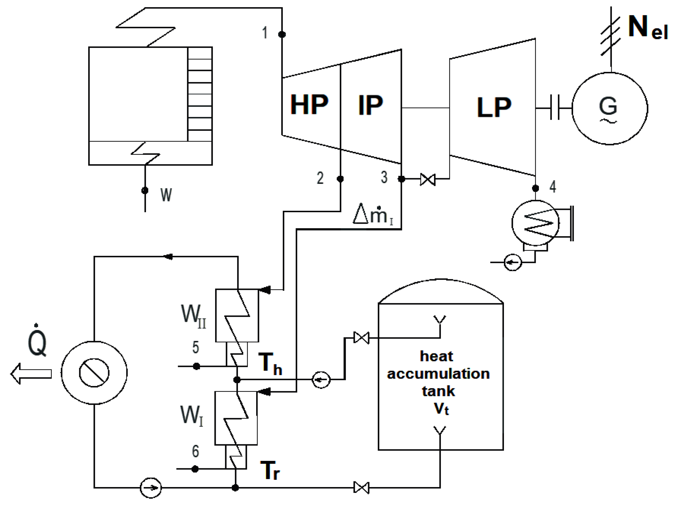
A heat accumulation tank (Figure 1) is capable of storing network hot water in the base load hours τ_a corresponding to the decreased electricity demand. Throughout this period, the additional amount of hot water can be accumulated and heated in the base load heater W_I (which requires an increase of the capacity of this heater) as a result of bleeding an increased volume of steam whose value is equal to Δṁ_I (Equation (5)). In the peak load period $({\tau }_D-{\tau }_a)$, the extraction designed to feed the W_I heater can be closed and the total steam that is extracted is routed into the condensing section of the turbine with the purpose of producing additional volumes of electricity, whereas the hot water stored in the accumulation tank can be used to feed the distribution network and supplement the demand for thermal power (Figure 4 and Figure 5).

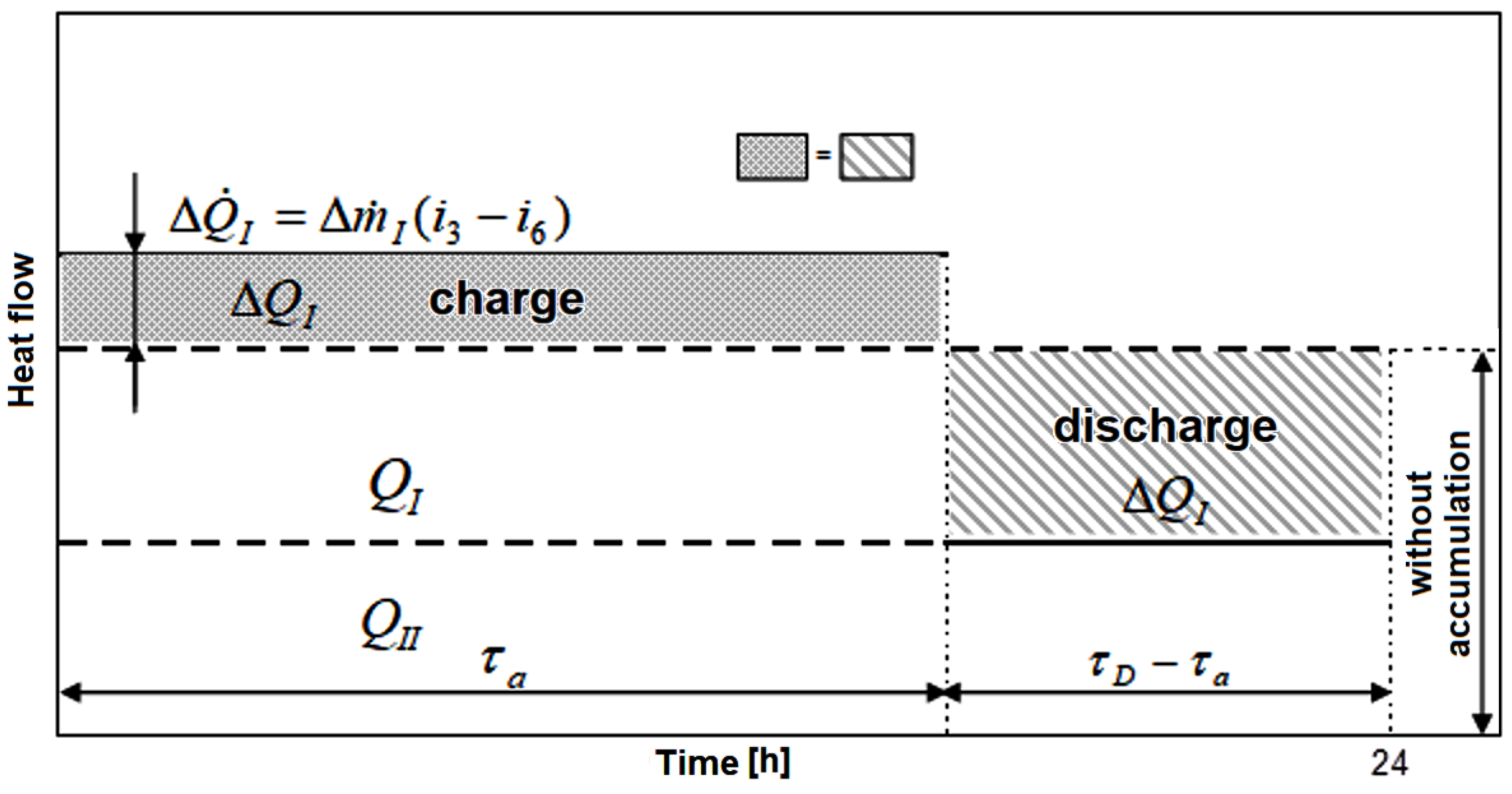
In a system excluding heat accumulation, the amount of heat that is transferred to the heat distribution network over the period of one day from the base load heater W_I (Figure 2 and Figure 3) is expressed by the formula:

$$Q_I={\dot{m}}_I(i_3-i_6){\tau }_D,$$

(3)

where ṁ_I—extraction steam flow rate routed into base load heater W_I in a system excluding accumulation, i₃—specific enthalpy of extraction steam prior to W_I heater, i₆—specific enthalpy of water behind W_I heater and ${\tau }_D$—number of hours in a day.

For the case of a system accounting for a heat accumulation tank, the same volume of heat Q_I can be derived from the following formula under the assumption that the W_I heater is excluded from operation in the peak period (Figure 3):

$$Q_I=({\dot{m}}_I+\Delta {\dot{m}}_I)(i_3-i_6){\tau }_a,$$

(4)

where τ_a—number of hours when heat accumulation tank is charged (i.e., number of hours in the base load period of the power system) and $\Delta {\dot{m}}_I$—increase of the steam flow extracted to feed W_I heater.

As a consequence, on the basis of (3) and (4), we can calculate the increase of steam flow extracted to feed W_I heater:

$$\Delta {\dot{m}}_I={\dot{m}}_I\frac{{\tau }_D-{\tau }_a}{{\tau }_a}.$$

(5)

On the basis of an energy balance of the base load heater W_I, we can derive the capacity V_t of the heat accumulation tank. If we disregard the heat losses into the atmosphere, this capacity is given by the expression:

$$V_t=\Delta {\dot{m}}_I{\tau }_a\frac{(i_3-i_6)}{{\rho }_w{c}_w(T_h-T_r)}$$

(6)

where ρ_w, c_w—density and specific heat capacity of water, and T_h, T_r—temperature of network hot water before and after it is heated (Figure 1).

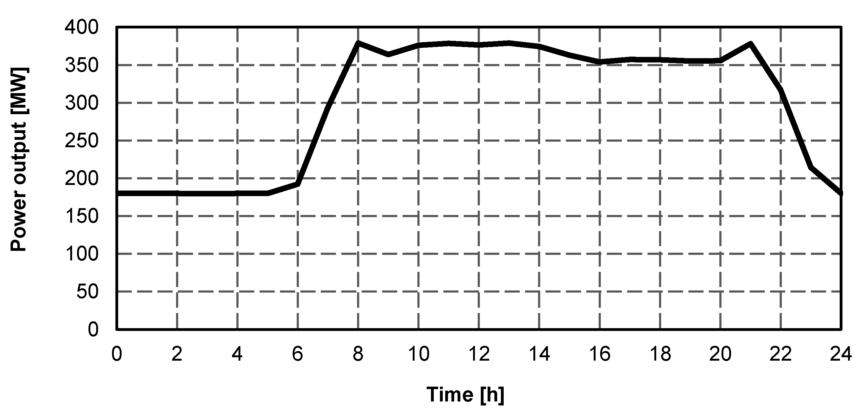
By analyzing the variability of the electrical capacity of the turbogenerator in the system comprising an accumulator with the one excluding it, we obtain the following formulae (Figure 4):

• for the base load period τ_a corresponding to the power system demand:

  $$\Delta N_{el}^{{\tau }_a}=-\Delta {\dot{m}}_I(i_3-i_4){\eta }_{me},$$

  (7)
• for the peak load period $({\tau }_D-{\tau }_a)$ corresponding to the power system demand:

  $$\Delta N_{el}^{{\tau }_D-{\tau }_a}={\dot{m}}_I(i_3-i_4){\eta }_{me}.$$

  (8)

  where i₄—specific enthalpy of the steam routed into the condenser and η_me—electromechanical efficiency of the turbogenerator.

2.2. Economic Analysis of Applying Heat Accumulation Tanks in CHP Plants

The necessary condition for securing the economic profitability of applying heat accumulators in CHP plants is associated with the condition that the profit from the exploitation of the modernized CHP plant does not decrease in relation to this profit before the process has been initiated. This condition is equivalent to the one that involves not increasing the cost of the heat production in the CHP plant. This cost is calculated in accordance with the methodology of the avoided cost, hence in a system comprising heat accumulation tank $K_h^{accu}$ this cost must not be greater from the cost of the system excluding accumulation K_h:

$$\begin{array}{l}{K}_h^{accu}=\frac{(z\rho +{\delta }_{serv}^{})(J^{CHP}+J^{accu})}{365}+{\displaystyle \sum K_e^{}}+K_P-(E_{el}+\Delta E_{el}^{accu})e_{el}\le \\ \\ \le K_h^{}=\frac{(z\rho +{\delta }_{serv}^{})J^{CHP}}{365}+{\displaystyle \sum K_e^{}}-E_{el}{e}_{el}\end{array}$$

(9)

where e_el—electricity price, $E_{el},\Delta E_{el}^{accu}$—production and increase in the net electricity production in the system comprising a heat accumulation tank per day, J^accu—turnkey investment in a heat accumulator (i.e., details of the value of investment J^accu and the cost structure can be found e.g., in [16]; this investment needs to include the resources needed for the increase of the capacity of the W_I heater), J^CHP—investment in the CHP plant before its modernization, ΣK_e—exploitation cost excluding cost of maintenance and overhaul of equipment per year, K_p—cost of electricity needed to drive the pumps coupled with the accumulation tank per day, zρ + δ_serv—annual rate (zρ) of handling capital investment (depreciation rate with interest [13,14]) and rate (δ_serv) of the remaining fixed cost relative to the investment (cost of maintenance and overhaul of equipment) [13,14,15,16], z—depreciation rate of the investment J^accu [13,14,15,16] and 365—number of days per year.

After the reduction of both terms on sides of Equation (9), we finally obtain only the increase in the revenues and costs related to the investment J^accu associated with the modernization: the increase of revenues $\Delta E_{el}^{accu}{e}_{el}$ from the sales of additional production of electricity, increase of the capital cost equal to zρJ^accu, increase in the maintenance and overhaul cost equal to δ_servJ^accu and cost K_p related to the electricity needed to power the new equipment—Equation (10). The incremental form of the Formula (10) is very beneficial and can be useful for analyzing the economic profitability of this modernization. As a result, we do not need the value of the past investment J^CHP and past revenues E_ele_el as well as capital cost zρJ^CHP and exploitation cost of the CHP plant δ_servJ^CHP, ΣK_e prior to its modernization. The accessibility of this data is additionally difficult or impossible to obtain as it forms trade secret or confidential commercial information. The incremental Equation (10) (and generally speaking, the incremental methodology [13,14,15]) offers a way in which the issues related to inaccessibility of the details regarding the period prior to the modernization can be dealt with so as to gain data regarding the economic profitability of the process without access to this information. We can emphasize that the economic analysis of the modernization is only possible after a prior thermodynamic analysis of the modernized power unit. The results of engineering criteria offer input values for the economic analysis. For example, the details of the increase in the electricity production $\Delta E_{el}^{accu}$ can be derived from the Equations (7) and (8) (Figure 4).

The condition necessary for securing the economic profitability of the use of heat accumulation tanks in CHP plants can be limited to the condition that the revenues from the sales of the electricity generated in the peak load is at least not smaller from the increase of the cost associated with the construction of the heat accumulation tank. This condition can be applied to determine the economically justified minimum difference between electricity prices at which is it sold to the distribution companies at the times when maximum electricity output is required. The maximum output in this case means only the increase the electricity production $\Delta N_{el}^{pl}$ of the power unit above its level determined as the base load (Figure 4).

When we take into account the above remarks, the necessary condition (9) providing the assessment of the economic profitability of the use of heat accumulation can be expressed by the following relation:

$$\begin{array}{l}\Delta {\dot{m}}_I(i_3-i_4){\eta }_{me}({\tau }_D-{\tau }_a)(e_{el}^{pl}-e_{el}^{bl})+{\dot{m}}_I(i_3-i_4){\eta }_{me}({\tau }_D-{\tau }_a)e_{el}^{pl}-\\ \\ \begin{array}{ccc}& & \end{array}-\Delta {\dot{m}}_I(i_3-i_4){\eta }_{me}{\tau }_a{e}_{el}^{bl}\ge \frac{(z\rho +{\delta }_{serv})J^{accu}}{365}+K_P,\end{array}$$

(10)

where $e_{el}^{bl},e_{el}^{pl}$—base load and peak load electricity prices.

The first term on the left-hand side of the relation in (10) denotes the increase of the revenues resulting only from the difference between the peak load and base load electricity prices (in a system excluding accumulation, the electricity $\Delta {\dot{m}}_I(i_3-i_4){\eta }_{me}({\tau }_D-{\tau }_a)$ is sold at a price equal to $e_{el}^{bl}$), the second term denotes the revenues from the sales of electricity at the prices from peak load and the third results from the decrease of the revenue from the sales of base load electricity in accordance with the power system power regulation schedule.

The terms on the right-hand side of the relation (10) denote the cost of capital (zρJ^accu/365) and exploitation (δ_servJ^CHP/365) + K_P) related to the operation of a heat accumulation tank.

By applying the relations (5), (6), (10) and the formula for the turnkey investment in the heat accumulation tank:

$$J^{accu}=V_t{i}_{V_t}$$

(11)

where $i_{V_t}$—specific investment in a heat accumulation tank (per unit of its capacity), and under the assumption that K_P ≅ 0, we are able to determine the necessary difference in the peak load and base load electricity price as given by power system:

$${(e_{el}^{pl}-e_{el}^{bl})}_{\min }^{}=\frac{(z\rho +{\delta }_{serv})i_{V_t}}{365{\eta }_{me}{\rho }_w{c}_w(T_h-T_r)}\frac{(i_3-i_6)}{(i_3-i_4)}\frac{{\tau }_a}{{\tau }_D}.$$

(12)

For instance, if we substitute the following values: c_w = 4.19 kJ/(kg∙K), i₃ = 2600, i₄ = 2355, i₆ = 305 kJ/kg, $i_{V_t}$ = 480 PLN/m³ (Vt = 3780 m³), T_h − T_r = 25 K, zρ + δ_serv = 14%/a, η_me = 0.95, ρ_w = 1000 kg/m³, ${\tau }_a/{\tau }_D$ ≅ 0.55 into Equation (12), we receive the condition that the minimum difference in the peak load and base load electricity prices should be equal to: ${(e_{el}^{pl}-e_{el}^{bl})}_{\min }^{}$ ≅ 35 PLN/MWh. For a pressure tank $i_{V_t}$ = 2725 PLN/m³ (Formulas (11) and (13)), the difference ${(e_{el}^{pl}-e_{el}^{bl})}_{\min }^{}$ is equal to as much as 197 PLN/MWh. These calculations apply the exchange rate of US dollar to Polish zloty equal to 1 USD = 3.6 PLN.

The turnkey investment in the heat accumulator is equal to [12]:

• for pressure tank:

  $$J_{press}^{accu}=48,281{(V_t)}^{0,4955}[\mathrm{USD}\mathrm{thousand}]$$

  (13)
• for non-pressure tank:

  $$J_{non-press}^{accu}=2,5083{(V_t)}^{0,6442}[\mathrm{USD}\mathrm{thousand}]$$

  (14)

  where the capacity V_t of the accumulator is expressed in m³. The investment includes: a steel tank (i.e., non-pressure or pressure tank), pipeline, armature, charge and discharge pumps (these can also be reversible ones) along with the motors and drives, metering and control systems, tank insulation, building and design cost (e.g., foundations), corrosion protection works and internal elements of a vessel, including a distribution system, diffusors, etc. The investment in the pressure tank is several times greater compared to the cost of non-pressure tank (as the superpressure in the range of around 300−500 Pa is used in the latter design). The construction period was taken to be equal to one year.

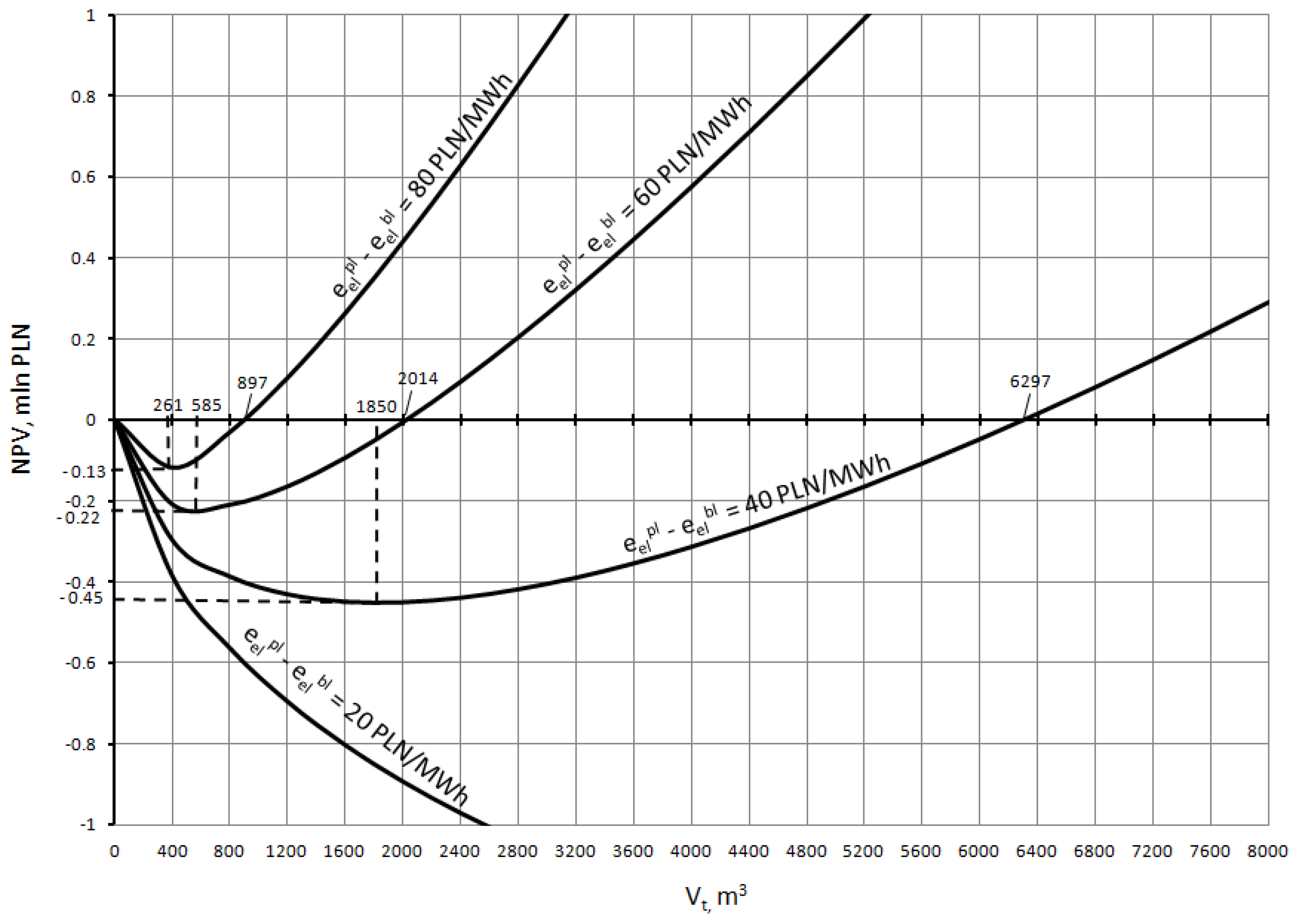
An important consideration which needs to be taken into account during the design phase of a heat accumulation tank combined with a CHP plant is associated with its optimal capacity $V_t^{opt}$, i.e., the capacity which guarantees the maximum possible profit from its exploitation. The search for this value should apply the criterion of the maximization of the cumulative, discounted NPV (Formula (28)) that is gained from the exploitation of a heat accumulation tank over the entire period when it is in operation expressed in a continuous time notation. Throughout the search for its capacity, it is necessary to express this profit as a function of the capacity NPV = f(V_t), and importantly, apply continuous time notation to find this profit [13,14,15,16,17]. This is due to the fact that the notation applying continuous time provides a way in which differential calculations can be used to find an extreme value of NPV. Thus, it is possible to explicitly assess the impact of the capacity V_t on the value of NPV, as well as find not only the optimum capacity $V_t^{opt}$, but also the region with the values that are close to this optimum. Moreover, this function can provide information regarding the characteristics of the variability of NPV in the function of V_t. In the present case, this profit expressed in the continuous time notation takes the form:

$$NPV={\displaystyle \underset{0}{\overset{T}{\int }}[\Delta S_A-\Delta K_e-F^{accu}-R^{accu}-(\Delta S_A-\Delta K_e-F^{accu}-A^{accu})p]{\mathrm{e}}^{-rt}}dt$$

(15)

where A^accu—depreciation rate, A^accu = J^accu/T [13,14,15,16,17], F^accu—time-variable interest (cost of finance) charged on the investment J^accu, F^accu = r[J^accu − (t − 1)R^accu] [13,14,15,16], ΔK_e—annual cost of maintenance and overhaul of a heat accumulator, p—income tax rate, R^accu—loan instalment, R^accu = J^accu/T [13,14,15,16,17], r—interest rate on capital $J^{accu}$, ΔS_A—time-variable increase of the annual revenue from the production of peak load electricity, t—time and T—exploitation period of a heat accumulator expressed in years,

Since heat production in the peak, heating season, i.e., winter is different from the value in the non-heating season, the annual increase of the revenue resulting from the production of net electricity in the peak load period in Formula (10) should be expressed by the relation:

$$\begin{array}{ll}\hfill \Delta S_A=& \{L_{heat}[\Delta {\dot{m}}_I^{heat}(i_3-i_4){\eta }_{me}({\tau }_D-{\tau }_a^{heat})(e_{el}^{pl}-e_{el}^{bl})+{\dot{m}}_I^{heat}(i_3-i_4){\eta }_{me}({\tau }_D-{\tau }_a^{heat})e_{el}^{pl}+\hfill \\ & -\Delta {\dot{m}}_I^{heat}(i_3-i_4){\eta }_{me}{\tau }_a^{heat}{e}_{el}^{bl}]+L_{non-heat}[\Delta {\dot{m}}_I^{non-heat}(i_3-i_4){\eta }_{me}({\tau }_D-{\tau }_a^{non-heat})(e_{el}^{pl}-e_{el}^{bl})+\hfill \\ & +{\dot{m}}_I^{non-heat}(i_3-i_4){\eta }_{me}({\tau }_D-{\tau }_a^{non-heat})e_{el}^{pl}-\Delta {\dot{m}}_I^{non-heat}(i_3-i_4){\eta }_{me}{\tau }_a^{non-heat}{e}_{el}^{bl}]\}(1-{\epsilon }_{el}),\hfill \end{array}$$

(16)

where L_heat—duration of the heating season, L_non-heat—number of days in the non-heating season, L_non-heat = 365 − L_heat, and ε_el—internal electrical load of the CHP plant.

In relation (16), it was assumed that the prices of the base load and peak load electricity are the same. The search for an optimum capacity $V_t^{opt}$ should apply the notation of all integrated functions in (15) in the function of V_t. For instance, in Equation (16), the following fluxes: $\Delta {\dot{m}}_I^{heat}$, $\Delta {\dot{m}}_I^{non-heat}$, ${\dot{m}}_I^{heat}$, ${\dot{m}}_I^{non-heat}$ need to be expressed in the function of V_t. For this purpose, it is necessary to apply Equations (3), (4) and (6) as well as find a relation to relate the weighted mean of heat $Q_I^{heat}$ that is transmitted into the distribution network per day in the peak season with the heat transmitted in the off-peak season $Q_I^{non-heat}$ only for the purposes of hot water production:

$$Q_I^{heat}=\beta Q_I^{non-heat}.$$

(17)

The heat in $Q_I^{heat}$ is many times greater from the one in $Q_I^{non-heat}$. The β parameter is in the range from around 3 to even 10. Consequently, the capacity V_t needs to be defined in terms of the heat in $Q_I^{heat}$:

$$V_t=\frac{Q_I^{heat}}{{\rho }_w{c}_w(T_h^{heat}-T_r^{heat})}(1-\frac{{\tau }_a^{heat}}{{\tau }_D}).$$

(18)

On the basis of Equations (3), (4) and (6), we can derive the dependencies expressing the fluxes $\Delta {\dot{m}}_I^{heat}$, ${\dot{m}}_I^{heat}$ in the function of the capacity V_t:

$$\Delta {\dot{m}}_I^{heat}=\frac{V_t{\rho }_w{c}_w(T_h^{heat}-T_r^{heat})}{(i_3-i_6){\tau }_a^{heat}},$$

(19)

$${\dot{m}}_I^{heat}=\frac{V_t{\rho }_w{c}_w(T_h^{heat}-T_r^{heat})}{(i_3-i_6)({\tau }_D-{\tau }_a^{heat})},$$

(20)

In addition, by applying the dependence in (17), we can derive the fluxes ${\dot{m}}_I^{non-heat}$, $\Delta {\dot{m}}_I^{non-heat}$:

$$Q_I^{non-heat}={\dot{m}}_I^{non-heat}(i_3-i_6){\tau }_D=\frac{Q_I^{heat}}{\beta }=\frac{{\dot{m}}_I^{heat}(i_3-i_6){\tau }_D}{\beta },$$

(21)

Hence, we obtain:

$${\dot{m}}_I^{non-heat}=\frac{{\dot{m}}_I^{non-heat}}{\beta }$$

(22)

and on the basis of the relation:

$$Q_I^{non-heat}=({\dot{m}}_I^{non-heat}+\Delta {\dot{m}}_I^{non-heat})(i_3-i_6){\tau }_a^{non-heat}=\frac{Q_I^{heat}}{\beta }=\frac{({\dot{m}}_I^{heat}+\Delta {\dot{m}}_I^{heat})(i_3-i_6){\tau }_a^{heat}}{\beta }$$

(23)

we get:

$$\Delta {\dot{m}}_I^{non-heat}=\frac{({\dot{m}}_I^{heat}+\Delta {\dot{m}}_I^{heat})}{\beta }\frac{{\tau }_a^{heat}}{{\tau }_a^{non-heat}}-\frac{{\dot{m}}_I^{heat}}{\beta }.$$

(24)

By expressing the investment in terms of the exponential function:

$$J^{accu}=\mathrm{A}{V}_t{}^{\mathrm{B}}$$

(25)

and as a result of expressing the annual cost of maintenance and overhaul of a heat accumulator in the form:

$$\Delta K_e={\delta }_{serv}{J}^{accu}$$

(26)

and by assuming the electricity price e_el by means of an exponential function (i.e., depending on the value $a_{el}$, the price e_el can increase, decrease or remain constant in the successive years):

$$e_{el}(t)=e_{el}^{t=0}{\mathrm{e}}^{a_{el}t}$$

(27)

and by substituting the following relations into Equation (15) and performing integration, we receive a formula that gives NPV which is gained from the exploitation of a heat accumulation tank in the function of its capacity V_t:

$$\begin{array}{cc}\hfill NPV=& \{\Delta E_{el,A}^1\left\{e_{el}^{pl,t=0}\frac{1}{a_{el}^{pl}-r}{[\mathrm{e}}^{(a_{el}^{pl}-r)T}-1]-e_{el}^{bl,t=0}\frac{1}{a_{el}^{bl}-r}{[\mathrm{e}}^{(a_{el}^{bl}-r)T}-1]\right\}+\hfill \\ & +\Delta E_{el,A}^2{e}_{el}^{pl,t=0}\frac{1}{a_{el}^{pl}-r}{[\mathrm{e}}^{(a_{el}^{pl}-r)T}-1]-\Delta E_{el,A}^3{e}_{el}^{bl,t=0}\frac{1}{a_{el}^{bl}-r}{[\mathrm{e}}^{(a_{el}^{bl}-r)T}-1]+\hfill \\ & +\Delta E_{el,A}^4\left\{e_{el}^{pl,t=0}\frac{1}{a_{el}^{pl}-r}{[\mathrm{e}}^{(a_{el}^{pl}-r)T}-1]-e_{el}^{bl,t=0}\frac{1}{a_{el}^{bl}-r}{[\mathrm{e}}^{(a_{el}^{bl}-r)T}-1]\right\}+\hfill \\ & +\Delta E_{el,A}^5{e}_{el}^{pl,t=0}\frac{1}{a_{el}^{sz}-r}{[\mathrm{e}}^{(a_{el}^{pl}-r)T}-1]-\Delta E_{el,R}^6{e}_{el}^{d,t=0}\frac{1}{a_{el}^d-r}{[\mathrm{e}}^{(a_{el}^d-r)T}-1]+\hfill \\ & -\mathrm{A}{V}_c{}^{\mathrm{B}}\left[(1-{\mathrm{e}}^{-rT})\frac{{\delta }_{serv}}{r^{}}+z\left(\frac{1-{\mathrm{e}}^{-rT}}{T}+1\right)\right]\}(1-p)\to \max \hfill \end{array}$$

(28)

where:

$$\Delta E_{el,A}^1=L_{heat}\frac{V_t{\rho }_w{c}_w(T_h^{heat}-T_r^{heat})}{(i_3-i_6){\tau }_a^{heat}}(i_3-i_4){\eta }_{me}({\tau }_D-{\tau }_a^{heat})(1-{\epsilon }_{el})$$

(29)

$$\Delta E_{el,A}^2=L_{heat}{V}_t{\rho }_w{c}_w(T_h^{heat}-T_r^{heat})\frac{(i_3-i_4)}{(i_3-i_6)}{\eta }_{me}(1-{\epsilon }_{el})$$

(30)

$$\Delta E_{el,A}^3=\Delta E_{el,A}^2=L_{heat}{V}_t{\rho }_w{c}_w(T_h^{heat}-T_r^{heat})\frac{(i_3-i_4)}{(i_3-i_6)}{\eta }_{me}(1-{\epsilon }_{el})$$

(31)

$$\begin{array}{l}\Delta E_{el,A}^4=L_{non-heat}\left\{[\frac{V_t{\rho }_w{c}_w(T_h^{heat}-T_r^{heat})}{\beta (i_3-i_6)({\tau }_D-{\tau }_a^{heat})}+\frac{V_t{\rho }_w{c}_w(T_h^{heat}-T_r^{heat})}{\beta (i_3-i_6){\tau }_a^{heat}}]\frac{{\tau }_a^{heat}}{{\tau }_a^{non-heat}}-\frac{V_t{\rho }_w{c}_w(T_h^{heat}-T_r^{heat})}{\beta (i_3-i_6)({\tau }_D-{\tau }_a^{heat})}\right\}\times \\ \begin{array}{ccc}\begin{array}{cc}& \end{array}& & \end{array}\times (i_3-i_4){\eta }_{me}({\tau }_D-{\tau }_a^{non-heat})(1-{\epsilon }_{el})\end{array}$$

(32)

$$\Delta E_{el,A}^5=L_{non-heat}\frac{V_t{\rho }_w{c}_w(T_h^{heat}-T_r^{heat})}{\beta (i_3-i_6)({\tau }_D-{\tau }_a^{heat})}(i_3-i_4){\eta }_{me}({\tau }_D-{\tau }_a^{non-heat})(1-{\epsilon }_{el})$$

(33)

$$\begin{array}{l}\Delta E_{el,A}^6=L_{non-heat}\left\{[\frac{V_t{\rho }_w{c}_w(T_h^{heat}-T_r^{heat})}{\beta (i_3-i_6)({\tau }_D-{\tau }_a^{heat})}+\frac{V_t{\rho }_w{c}_w(T_h^{heat}-T_r^{heat})}{\beta (i_3-i_6){\tau }_a^{heat}}]\frac{{\tau }_a^{heat}}{{\tau }_a^{non-heat}}-\frac{V_t{\rho }_w{c}_w(T_h^{heat}-T_r^{heat})}{\beta (i_3-i_6)({\tau }_D-{\tau }_a^{heat})}\right\}\times \\ \begin{array}{ccc}\begin{array}{cc}& \end{array}& & \end{array}\times (i_3-i_4){\eta }_{me}{\tau }_a^{non-hear}(1-{\epsilon }_{el}).\end{array}$$

(34)

The second derivative of NPV with respect to V_t is equal to:

$$d^{2}NPV/d{V}_c^2=-\mathrm{AB}(\mathrm{B}-1)(V_t{)}^{\mathrm{B}-2}[(1-{\mathrm{e}}^{-rT})\frac{{\delta }_{serv}}{r^{}}+z(\frac{1-{\mathrm{e}}^{-rT}}{T}+1)](1-p)>0$$

(35)

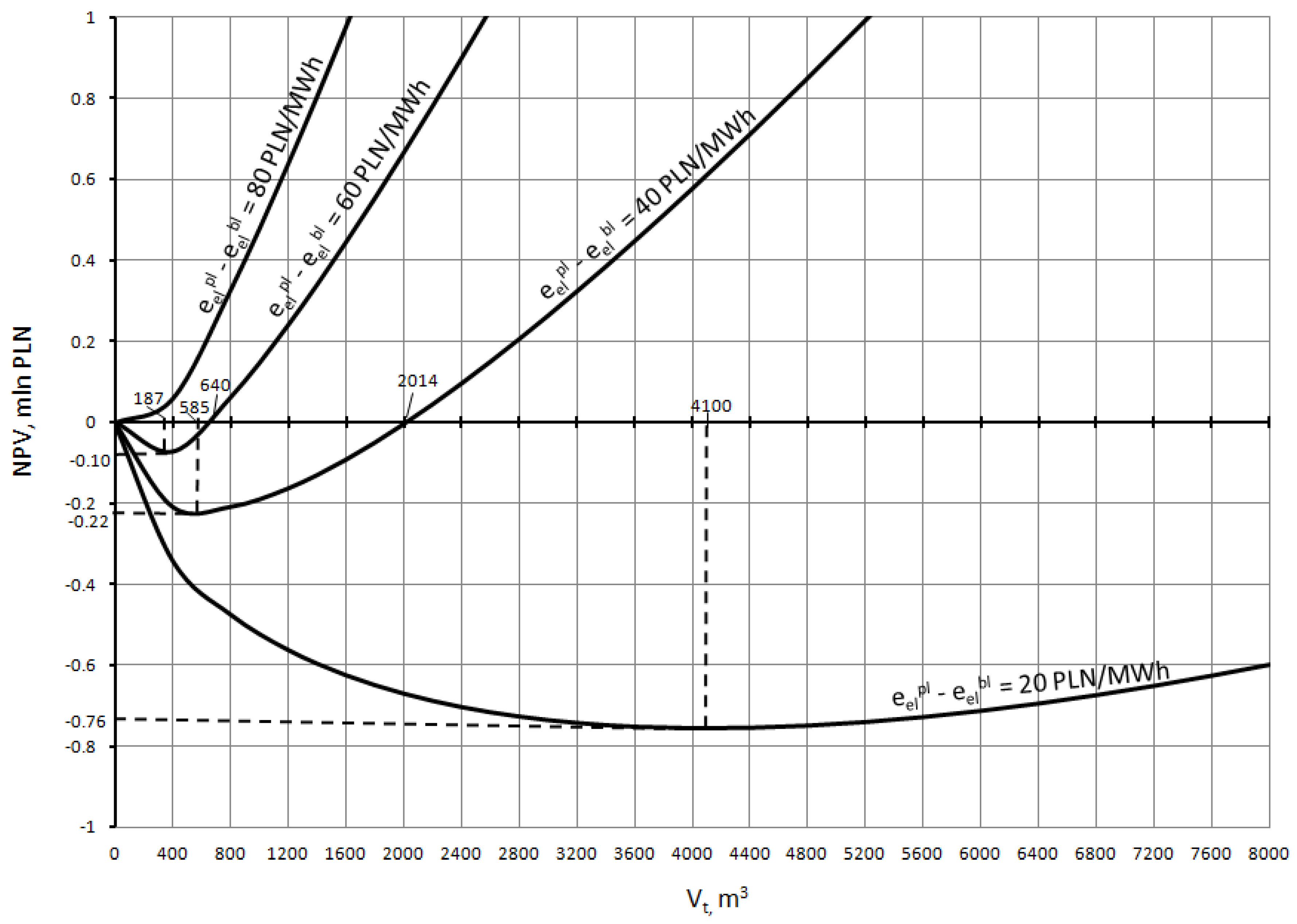
and it assumes only positive values, as we can see from (35), due to the fact that the values of the B coefficient are in the range B∈(0;1) (Equations (13) and (14)). Hence, the function of NPV = f(V_t) is concave in the entire range of the variability of the capacity V_t ∈ $\langle 0;\infty )V_t\in \langle 0;\infty )$ and assumes a minimum which always takes on a negative value: NPV_min = f($V_t^{\min }$) < 0, which can be concluded from the relation found in (36). Therefore, the function NPV = f(V_t) decreases constantly in the range $V_t\in \langle 0;V_t^{\min })$ and increases steadily in the range $V_t\in (V_t^{\min };\infty )$—Figure 5 and Figure 6. Hence, the value of NPV tends to infinity in the conditions when the capacity V_t tends to infinity: NPV → $\infty$, when V_t → $\infty$. The value $V_t^{\min }$ is derived on the basis of the necessary condition associated with the existence of an extreme of dNPV/dV_t—Equation (36).

After the substitution of Equations (29)–(34) into (28), the capacity of the heat accumulation tank $V_t^{\min }$ for which the profit assumes a minimum, i.e., NPV = NPV_min = f($V_t^{\min }$), can be derived on the basis of the following relation:

$$\begin{array}{c}{L}_{heat}{\rho }_w{c}_w(T_h^{heat}-T_r^{heat})\frac{i_3-i_4}{i_3-i_6}\frac{{\tau }_D}{{\tau }_a^{heat}}{\eta }_{me}(1-{\epsilon }_{el})\left[e_{el}^{pl,t=0}\frac{{\mathrm{e}}^{(a_{el}^{pl}-r)T}-1}{a_{el}^{pl}-r}-e_{el}^{bl,t=0}\frac{{\mathrm{e}}^{(a_{el}^{bl}-r)T}-1}{a_{el}^{bl}-r}\right]+\hfill \\ +L_{non-heat}\left\{\left[\frac{{\rho }_w{c}_w(T_h^{heat}-T_r^{heat})}{\beta (i_3-i_6)({\tau }_D-{\tau }_a^{heat})}+\frac{{\rho }_w{c}_w(T_h^{heat}-T_r^{heat})}{\beta (i_3-i_6){\tau }_a^{heat}}\right]\frac{{\tau }_a^{heat}}{{\tau }_a^{non-heat}}-\frac{{\rho }_w{c}_w(T_h^{heat}-T_r^{heat})}{\beta (i_3-i_6)({\tau }_D-{\tau }_a^{heat})}\right\}\times \hfill \\ \times (i_3-i_4){\eta }_{me}({\tau }_D-{\tau }_a^{non-heat})(1-{\epsilon }_{el})\left[e_{el}^{pl,t=0}\frac{{\mathrm{e}}^{(a_{el}^{pl}-r)T}-1}{a_{el}^{pl}-r}-e_{el}^{bl,t=0}\frac{{\mathrm{e}}^{(a_{el}^{bl}-r)T}-1}{a_{el}^{bl}-r}\right]+\hfill \\ +L_{non-heat}{\rho }_w{c}_w(T_h^{heat}-T_r^{heat})\frac{(i_3-i_4)({\tau }_D-{\tau }_a^{non-heat})}{\beta (i_3-i_6)({\tau }_D-{\tau }_a^{heat})}{\eta }_{me}(1-{\epsilon }_{el})e_{el}^{pl,t=0}\frac{{\mathrm{e}}^{(a_{el}^{pl}-r)T}-1}{a_{el}^{pl}-r}+\hfill \\ -L_{non-heat}\left\{\left[\frac{{\rho }_w{c}_w(T_h^{heat}-T_r^{heat})}{\beta (i_3-i_6)({\tau }_D-{\tau }_a^{heat})}+\frac{{\rho }_w{c}_w(T_h^{heat}-T_r^{heat})}{\beta (i_3-i_6){\tau }_a^{heat}}\right]\frac{{\tau }_a^{heat}}{{\tau }_a^{non-heat}}-\frac{{\rho }_w{c}_w(T_h^{heat}-T_r^{heat})}{\beta (i_3-i_6)({\tau }_D-{\tau }_a^{heat})}\right\}\times \hfill \\ \times (i_3-i_4){\eta }_{me}{\tau }_a^{non-heat}(1-{\epsilon }_{el})e_{el}^{bl,t=0}\frac{{\mathrm{e}}^{(a_{el}^{bl}-r)T}-1}{a_{el}^{bl}-r}+\hfill \\ -\mathrm{AB}(V_c^{\min }{)}^{\mathrm{B}-1}\left[(1-{\mathrm{e}}^{-rT})\frac{{\delta }_{serv}}{r^{}}+z\left(\frac{1-{\mathrm{e}}^{-rT}}{T}+1\right)\right]=0.\hfill \end{array}$$

(36)

As we can find from (36), the value $V_t^{\min }$ increases along with the decrease of the value of $e_{el}^{pl}-e_{el}^{bl}.$

3. Results

Figure 5 and Figure 6 present the curves representing NPV in the function of the capacity of the heat accumulation tank V_t taking into account the parameter given by the electricity price $e_{el}^{pl}-e_{el}^{bl}$. The values of $V_t^{\min }$ in these two figures are equal to: $V_t^{\min }$ = 261 m³ for $e_{el}^{pl}-e_{el}^{bl}$ = 80 PLN/MWh, $V_t^{\min }$ = 585 m³ for $e_{el}^{pl}-e_{el}^{bl}$ = 60 PLN/MWh, $V_t^{\min }$= 1850 m³ for $e_{el}^{pl}-e_{el}^{bl}$ = 40 PLN/MWh as well as $V_t^{\min }$ = 12,830 m³ for $e_{el}^{pl}-e_{el}^{bl}$ = 20 PLN/MWh. Figure 5 and Figure 6 were developed for the case of the non-pressure heat accumulation tank, i.e., for the value of the investment given by Equation (14). Provided that the input data for the pressure accumulation tank are the same as for non-pressure one, these curves assume negative values of NPV for the actual, i.e., practically feasible, variability of the range of the capacity V_t, i.e., dimensions of the accumulation tank that do not exceed technically reasonable values. The alternative in which NPV assumes positive values for acceptable dimensions of the heat accumulation tank are expressed by the difference $e_{el}^{pl}-e_{el}^{bl}$ that would have to be several times greater from the difference with regard to a non-pressure tank. This results from several times greater investment needed in the pressure tank, expressed by Equation (13). The calculations in this case adopted the following input data: $a_{el}^{pl}=a_{el}^{bl}$ = 0, i₃ = 2600 kJ/kg, i₄ = 2355 kJ/kg, i₆ = 305 kJ/kg, L_heat = 225 days, p = 19%, r = 6%, T = 15 years, $T_h^{heat}-T_r^{heat}$ = 25 K, z = 1.03, β = 5, δ_serv = 3%, ε_el = 7%, η_me = 95%, ${\tau }_a^{heat}$ = 12 h, ${\tau }_a^{heat}={\tau }_a^{non-heat}$.

As we can find out from the curves in Figure 5 and Figure 6, NPV_max assumes its highest values for the greatest capacity of the tank V_t. In practice, however, this capacity V_t is limited for obvious reasons. The greatest value, now called the optimum capacity $V_t^{opt}$, is taken on in the conditions of the maximum possible increase of the steam extraction $\Delta {\dot{m}}_{I\max }^{heat}$ that can be applied to feed the W_I heater (Equation (6)):

$$V_t^{opt}=\frac{\Delta {\dot{m}}_{I\max }^{heat}{\tau }_a^{heat}(i_3-i_6)}{{\rho }_w{c}_w(T_h^{heat}-T_r^{heat})}.$$

(37)

A greater value of $\Delta {\dot{m}}_{I\max }^{heat}$ leads to the increase of the value of $V_t^{opt}$; consequently, the value of NPV_max increases as well. The value of NPV_max also increases following the greater difference in the prices $e_{el}^{pl}-e_{el}^{bl}$ (Figure 6 and Figure 7). The value of $\Delta {\dot{m}}_{I\max }^{heat}$ is relative to the thermal energy output from a CHP plant, which means that it also depends on the mass flow rate of steam ṁ₁ that is routed to the steam turbine installed in it. The maximum possible increase of the mass flow rate $\Delta {\dot{m}}_{I\max }^{heat}$ has an upper boundary given by the minimum flow rate of steam ṁ₄ that needs to be routed into the condenser in the turbine—Figure 1. This is due to the fact that this steam is responsible for the necessary cooling of the final section of the low-pressure turbine stage and needs to assume an adequately high value so as not to allow the ventilation work of this final section of the low-pressure turbine. Such a minimum flow rate of steam is taken to be equal to around 10% of the mass flow ${\dot{m}}_1$ that is routed into the high-pressure turbine stage—Figure 1. If the flow rate $\Delta {\dot{m}}_{I\max }^{heat}$ is so small that for the price difference $e_{el}^{pl}-e_{el}^{bl}$ that is possible to secure on the electricity market, as well as the capacity $V_t^{opt}$ derived from Equation (37) is smaller than the boundary value $V_t^{\lim }$ (that is, the value for which NPV is equal to zero, these boundary values are as follows: $V_t^{\lim }$ = 897 m³ for $e_{el}^{pl}-e_{el}^{bl}$ = 80 PLN/MWh, $V_t^{\lim }$ = 2014 m³ for $e_{el}^{pl}-e_{el}^{bl}$ = 60 PLN/MWh, $V_t^{\lim }$ = 6297 m³ for $e_{el}^{pl}-e_{el}^{bl}$ = 40 PLN/MWh and $V_t^{\lim }$ = 44,176 m³ for $e_{el}^{pl}-e_{el}^{bl}$ = 20 PLN/MWh), in this case the construction of the heat accumulation tank is not feasible from the economic viewpoint since the value of NPV is negative, i.e., NPV = f($V_t^{opt}$) < 0—see Figure 5 and Figure 6. If this difference is only equal to as little as $e_{el}^{pl}-e_{el}^{bl}$ = 20 PLN/MWh, the construction of the heat accumulation tank is not economically feasible.

For example for the value of $V_t^{opt}$ = 16,500 m³ resulting from the thermal capacity of the CHP plant (Equation (37)), which is a value that is below the boundary one equal to $V_t^{\lim }$ = 44,176 m³, this is the case. In such circumstances, the value of the profit is negative and equal to NPV = −1.54 mln PLN—Figure 5. This venture would be profitable for the price difference equal to $e_{el}^{pl}-e_{el}^{bl}$ = 40 PLN/MWh and this pertains even more for the price difference equal to $e_{el}^{pl}-e_{el}^{bl}$ = 60 PLN/MWh. In these two alternatives, the vales of the profit are positive and equal to NPV_max = 2.13 mln PLN and NPV_max = 5.8 mln PLN, respectively.

Figure 7, Figure 8, Figure 9 and Figure 10 demonstrate how the values of NPV and $V_t^{\lim }$ are affected by the number of hours ${\tau }_a$ when the heat accumulation tank is loaded. The calculations were performed for ${\tau }_a=8\mathrm{h}$ and ${\tau }_a=10\mathrm{h}$. Throughout this process, it was assumed that the remaining input characteristics assume the same values as for the case of the calculations presented in Figure 5. As we can see from the curves, the impact of the number of hours ${\tau }_a$ is very significant. The lower value of ${\tau }_a$ is accompanied by an increase of value of NPV and a decrease in the value of $V_t^{\lim }$. However, the minimum value of ${\tau }_a^{\min }$ is limited by the value of the mass flow $\Delta {\dot{m}}_{I\max }^{heat}$ that can be potentially obtained in accordance with Equation (5).

$${\tau }_a^{\min }=\frac{{\dot{m}}_I}{\Delta {\dot{m}}_{I\max }^{heat}+{\dot{m}}_I}{\tau }_D$$

(38)

By substituting Equation (38) to (37), the necessary condition for the profitability of heat accumulation tank operation can be written in dependence:

$$V_t^{opt}=\frac{\Delta {\dot{m}}_{I\max }^{heat}{\dot{m}}_I}{\Delta {\dot{m}}_{I\max }^{heat}+{\dot{m}}_I}\frac{(i_3-i_6)}{{\rho }_w{c}_w(T_h^{heat}-T_r^{heat})}{\tau }_D\ge V_t^{\lim }$$

(39)

wherein $V_t^{\lim }$ is determined from Equation (28) assuming that NPV = 0.

4. Conclusions

The novel methodology using continuous time notation applied in the papers [13,15,16] offers a completely new quality of economic analysis with regard to all technical processes. Its application in the search for an optimum capacity $V_t^{opt}$ of the heat accumulation tank combined with a CHP plant (Equation (15)) provided the way in which the maximum value of the $NPV=f(V_t^{})$ function could be derived (Equation (28)). This calculation provides insight into the maximum potential profit $NP{V}_{\max }$ gained from the exploitation of the heat accumulation tank. It is very important since the knowledge of its course over the entire range of the variability of the capacity $V_t\in \langle 0;\infty )$—Figure 5, Figure 7 and Figure 9—offers a comprehensive overview of the investigated problem. The familiar and commonly applied discreet notation of the NPV parameter [13,14,15,16] (with the discretization step of equal to one year) does not offer such an opportunity. Its application to calculate a few and even several values of NPV does not offer the assessment of the characteristics of the curve of NPV. Hence, he results expressed on the point scale do not offer the way in which such generalizations can be made and only the way from the general to the detail offers the possibility of stating general conclusions. Equally important, we can note that it was possible to derive Equations (37), (39) on the basis of the applied novel methodology. In addition, this formulas has a general application. Thus, it is possible to find an optimum capacity of a heat accumulation tank to suit every CHP plant design, whether it is a plant operating according to the block mode, where a boiler is assigned to a turbine, as in Figure 1, or the design comprising a steam header. Another important consideration resulting from the application of the continuous notation is association with the fact that the quantities needed to calculate $V_t^{opt}$ only include the specific steam enthalpies $i_3,i_6$—Figure 1—and the mass flow $\Delta {\dot{m}}_{I\max }^{heat}$. There is one more important thing to consider. If the optimal capacity $V_t^{opt}$ of a heat accumulation tank combined with a CHP plant corresponding to the potential and possible price difference $e_{el}^{pl}-e_{el}^{bl}$ gained in the electricity market derived from Equation (25) is smaller from the boundary value $V_t^{\lim }$ (i.e., the value corresponding to NPV value equal to zero, Figure 5, Figure 7 and Figure 9—Equation (37)), the construction of the heat accumulation tank is not economically feasible. The investment in such a heat accumulation tank is only feasible for the case when the difference $e_{el}^{pl}-e_{el}^{bl}$ between the peak load and base load electricity prices in the PPS is sufficiently high so as to guarantee that $NPV=f(V_t^{opt})>0$. This price difference, along with the value of the investment $J^{accu}$ and possible to obtain in CHP plant value $\Delta {\dot{m}}_{I\max }^{heat}$ form the factors which determine the economic justification of building a heat accumulation tank. Finally, we can emphasize that for the case of a CHP plant operating in a system coupled by a steam header, i.e., for the case when the boiler(s) have a common header, which is routed steam into a number of turbines followed by steam extraction into low-pressure pipes from the turbine exhausts, the mass flow from collected from them $\Delta {\dot{m}}_{I\max }^{heat}$ is to a considerably smaller extent limited in comparison to the block mode. Hence, this value can be greater. The layouts comprising a steam header are usually built in industrial CHP plants, in which there is a demand for heat at various temperature levels and the processes applied the need to involve low-pressure headers with various pressure levels. The system connected by a header is more expensive in comparison to the layout built in the block mode, as the latter provides a manner to control the operation of the boilers and turbines in a CHP plant.

References

1. Beckmann, G.; Gilli, P.V. Thermal Energy Storage; Springer: Wien, Austria, 1984. [Google Scholar]
2. Bogdan, Ž.; Kopjar, D. Improvement of the cogeneration plant economy by using heat accumulator. Energy 2006, 31, 2285–2292. [Google Scholar] [CrossRef]
3. Christidis, A.; Koch, C.; Pottel, L.; Tsatsaronis, G. The contribution of heat storage to the profitable operation of combined heat and power plants in liberalized electricity markets. Energy 2012, 41, 75–82. [Google Scholar] [CrossRef]
4. Constantin, L.; Stanciu, D.; Crismaru, I. Optimization of heat exchange in a heat accumulator with latent heat storage. Procedia Technol. 2015, 19, 737–741. [Google Scholar] [CrossRef]
5. Hazami, M.; Kooli, S.; Naili, N.; Mehdaoui, F.; Guizani, A. Energy, exergy and economic viability of a heat storage system used for domestic hot water supply in urban and isolated households. Appl. Therm. Eng. 2017, 124, 442–453. [Google Scholar] [CrossRef]
6. Korpela, T.; Kaivosoja, J.; Majanne, Y.; Laakkonen, L.; Nurmoranta, M.; Vilkko, M. Utilization of District Heating Networks to Provide Flexibility in CHP Production. Energy Procedia 2017, 116, 310–319. [Google Scholar] [CrossRef]
7. Milewski, J.; Bujalski, W. STES—Typical scenarios for heat accumulator cooperation. Energy Procedia 2014, 50, 414–420. [Google Scholar] [CrossRef]
8. Romanovsky, G.; Mutale, J. Implementation of heat production and storage technology and devices in power systems. Appl. Therm. Eng. 2012, 48, 296–300. [Google Scholar] [CrossRef]
9. Short, M.; Crosbie, T.; Dawood, M.; Dawood, N. Load forecasting and dispatch optimisation for decentralized co-generation plant with dual energy storage. Appl. Energy 2017, 186, 304–320. [Google Scholar] [CrossRef]
10. Streckiene, G.; Martinaitis, V.; Andersen, A.N.; Katz, J. Feasibility of CHP-plants with thermal stores in the German spot market. Appl. Energy 2009, 86, 2308–2316. [Google Scholar] [CrossRef]
11. Zhang, H.; Baeyens, J.; Caceres, G.; Degreve, J.; Lv, J. Thermal energy storage: Recent developments and practical aspects. Prog. Energy Combust. Sci. 2016, 53, 1–40. [Google Scholar] [CrossRef]
12. Zuwała, J. Akumulacja Ciepła w Elektrociepłowniach w Aspekcie Dodatkowej Produkcji Szczytowej Energii Elektrycznej. Rozprawa Doktorska, Wydział Inżynierii Środowiska i Energetyki, Politechnika Ślaska, Gliwice, Poland, 2003. (In Polish). [Google Scholar]
13. Bartnik, R.; Buryn, Z.; Hnydiuk-Stefan, A. Ekonomika Energetyki w Modelach Matematycznych z Czasem Ciągłym; Wydawnictwo Naukowe PWN: Warszawa, Poland, 2017. (In Polish) [Google Scholar]
14. Bartnik, R.; Bartnik, B. Rachunek Ekonomiczny w Energetyce; Wydawnictwo WNT: Warszawa, Poland, 2014. (In Polish) [Google Scholar]
15. Bartnik, R.; Buryn, Z.; Hnydiuk-Stefan, A. Investment Strategy in Heating and CHP. Mathematical Models; Springer: London, UK, 2017. [Google Scholar]
16. Bartnik, R.; Bartnik, B.; Hnydiuk-Stefan, A. Optimum Investment Strategy in the Power Industry. Mathematical Models; Springer: New York, NY, USA, 2016. [Google Scholar]
17. Bartnik, R.; Hnydiuk-Stefan, A.; Buryn, Z. Analysis of the impact of technical and economic parameters on the specific cost of electricity production. Energy 2018, 147, 965–979. [Google Scholar] [CrossRef]
Figure 1. Diagram of a CHP (combined heat and power) plant comprising a heat accumulation tank.
Energies 11 01240 g001
Figure 2. Standard, actual daily course of the variability of electrical power output from a CHP plant.
Energies 11 01240 g002
Figure 3. Thermal load of the CHP plant comprising a heat accumulation tank.
Energies 11 01240 g003
Figure 4. Electrical load of the CHP plant comprising a heat accumulation tank.
Energies 11 01240 g004
Figure 5. Net Present Value (NPV) in the function of the capacity of the heat accumulation tank for τa = 12 h.
Energies 11 01240 g005
Figure 6. Enlarged details from Figure 5.
Energies 11 01240 g006
Figure 7. Net Present Value (NPV) in the function of the capacity of the heat accumulation tank for τa = 8 h.
Energies 11 01240 g007
Figure 8. Enlarged details from Figure 7.
Energies 11 01240 g008
Figure 9. Net Present Value (NPV) in the function of the capacity of the heat accumulation tank for τ a = 10 h .
Energies 11 01240 g009
Figure 10. Enlarged details from Figure 9.
Energies 11 01240 g010