Microgrids Real-Time Pricing Based on Clustering Techniques


1
Jiangsu Province Laboratory of Mining Electric and Automation, China University of Mining and Technology, Xuzhou 221000, China
2
Ernst & Young, Brisbane QLD 4000, Australia
*
Author to whom correspondence should be addressed.
Energies 2018, 11(6), 1388; https://doi.org/10.3390/en11061388
Submission received: 1 May 2018
/
Revised: 20 May 2018
/
Accepted: 21 May 2018
/
Published: 30 May 2018
(This article belongs to the Special Issue Distribution System Operation and Control)
Abstract
:Microgrids are widely spreading in electricity markets worldwide. Besides the security and reliability concerns for these microgrids, their operators need to address consumers’ pricing. Considering the growth of smart grids and smart meter facilities, it is expected that microgrids will have some level of flexibility to determine real-time pricing for at least some consumers. As such, the key challenge is finding an optimal pricing model for consumers. This paper, accordingly, proposes a new pricing scheme in which microgrids are able to deploy clustering techniques in order to understand their consumers’ load profiles and then assign real-time prices based on their load profile patterns. An improved weighted fuzzy average k-means is proposed to cluster load curve of consumers in an optimal number of clusters, through which the load profile of each cluster is determined. Having obtained the load profile of each cluster, real-time prices are given to each cluster, which is the best price given to all consumers in that cluster.
1. Introduction
1.1. Background, Motivations and Aims
Microgrids are expected to play a key role in future electricity markets, either as islanded or connected to the main grid. Microgrid operators are then responsible for delivering energy to consumers while meeting technical and economic criteria. One key issue for microgrid operator is determining proper pricing tariffs for consumers. One way is deploying the traditional flat prices for all consumers, which is deemed to be an inefficient pricing in electricity markets. An alternative is to define various price tariffs like time of use or even real-time prices. To this end microgrid operators need to understand their consumers’ characteristics so as they can assign optimal pricing schemes to various consumers.
Clustering techniques are known as a suitable method for load profiling according to load patterns of consumers, which help find the key characteristics of consumers. Consumers are clustered in various groups per their load pattern similarities. These techniques are indeed used for load profiling of consumers, where several applications such as future investments and planning are some.
This paper aims at determining optimal pricing schemes for microgrid considering load profile of consumers. To this end, an improved WFA k-means is proposed to accurately cluster consumers in several groups. These techniques cluster consumers based on their load similarities in each time interval for the entire day. Further, a similarity index, i.e., clustering dispersion indicator, is used to find the optimal number of clusters, which delivers the clusters with most similarities, but most difference with other clusters. Having the best cluster numbers, a load profile for each cluster is identified. This load profile is then used as a representative profile (RP) for all consumers in the given cluster. After that, microgrid operator deploys these representative profiles to determine price schemes for the consumers in each cluster.
1.2. Literature Review and Contributions
Research on microgrids has received a great deal of attention in recent years. An overview of microgrids control and energy management is given in [1]. A new model for plug-in or plug-out microgrids is presented in [2], where a hybrid interactive communication optimization solution is developed for optimal power dispatch of multiple microgrids. Technical issues of microgrids are addressed in several papers such as [3,4,5,6,7].
In terms of economic aspects of microgrids, studies such as energy scheduling by microgrids [8,9] and renewable energy in microgrids [10,11] are presented. Optimal renewable energy integration in microgrids is addressed in [12]. Authors in [13] proposes a new model for enabling demand response by microgrids. A chance-constrained approach is used in [14] in order to model microgrid scheduling. Although several papers address the economic modelling of microgrids, they mainly focus on the high-level and wholesale modelling of these grids and pay less attention on how to offer optimal prices to consumers. This is indeed an area this paper contributes over the existing studies.
In regards to clustering applications in power systems, most studies consider these techniques for load profiling [15,16,17,18,19]. These papers mostly use the basic clustering techniques such as k-means or the heuristic methods to classify load curves of consumers in several groups. Some drawbacks that these traditional clustering techniques have include randomly selecting the initial cluster centers which affect the final clustering result. Further, they mostly use the Euclidean distance measure for the computation of distance between data, which is not the accurate method for this purpose. This is the second area of our contributions.
Overall, this paper contributes over the existing studies in following aspects.
- This paper proposes a clustering-based pricing scheme for microgrids through which a microgrid operator can assign proper price tariffs on its consumers based on the load curves clustered in distinctive classes.
- As for clustering techniques, this paper applies an improved weighted fuzzy average k-means to overcome the drawbacks of the traditional k-means techniques.
The rest of the paper is in the following order. Section 2 describes the methodology framework, including the two-step framework, the clustering process and the procedure to achieve representative profiles (RPs) of consumers. Numerical results are presented in Section 3, where the case study is defined and several results are presented and then the scenarios for pricing schemes by microgrid operators are discussed. Conclusions are finally given in Section 4.
2. Methodology Framework
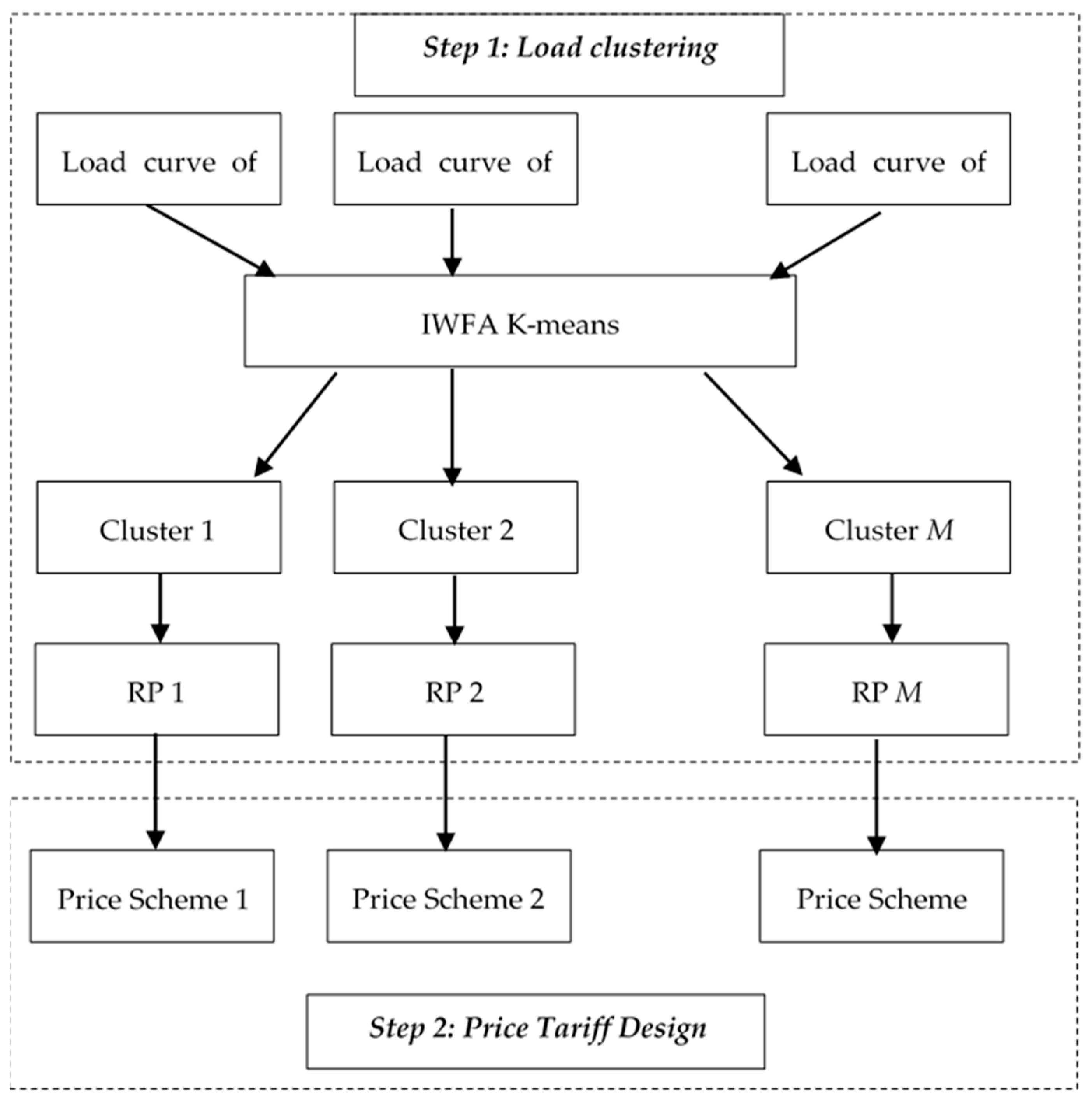
The proposed pricing scheme is provided in two steps. The first step accounts for consumers’ load clustering and deriving the representative load profile of each cluster. Then, in the second step, the microgrid operator deploys the outcome of the first step in order to design its proper pricing according to its requirements. Figure 1 illustrates the proposed two-step pricing scheme.
Each step is discussed in detail in following subsections.
2.1. Clustering Process
The load clustering procedure includes four steps as follows. The first step accounts for the selection of the proper data, e.g., load profiles of consumers in similar voltage levels, areas and within a distinctive network location. Once the data is collected, the next step ensures data processing. In this phase, outliers in the data are identified and removed. Step 3 includes load curve clustering, where the proposed clustering technique is carried out on consumers’ load profile and then using the adequacy measures such as CDI, the best number of clusters are chosen. Lastly, the representative profile (RP) of each cluster is determined by identifying the center of the relevant cluster. RPs are indeed useful to represent the further distinctive actions, pricing schemer here, which can be carried out on the consumers in each cluster.
This paper proposes the improved weighted fuzzy average (IWFA) k-means as follows. The traditional k-means has the following procedure. According the Euclidean distance, the data are clustered in several classes. The data in each cluster have common features but different from other clusters. It starts with an initial clustering and defines initial clusters, then iterates the approach until reach a final minimum difference in threshold of the two consecutive iterations.
One issue in k-means clustering to be considered is the simple averaging method which is used for cluster centers. Medians have shown better performance than averages, although they may remove good points. To overcome this issue, a type of fuzzy averaging is employed that puts the center prototype among the more densely situated points [2,9].
Consider {l(1),…, l(p)} as a set of p numbers. The algorithm initially considers the sample mean µ(0) and variance σ2 to start the process, to determine the weighted fuzzy average. Considering a vector of L with H components, the cluster center is calculated as follows:
This algorithm computes σ2 on several iterations and then uses it as a fixed number. This could lead to a sufficiently close WFA.
Further, using the Euclidean distance in the traditional k-means does not have proper accuracy. To resolve this issue, a new distance computation method is applied which ensure having more similar load curves in each cluster. To this end, the distance is computed using Equation (3), which weights the components of load curves based on their variance distinction.
Moreover, since the traditional k-means uses initial cluster centers randomly, the accuracy of load clustering is jeopardized. As such, the following equation is used to compute the initial cluster centers.
The method is iterated for different a and b to find the optimal outcome for clustering load curves.
There are several adequacy measures such as CDI, which allow us to determine the optimal number of clusters. Indeed, as the number of cluster declines, lower similarities in each cluster are witnessed. Extremely, for cluster number equals to 1, all load curves are grouped in one cluster, which has the lowest accuracy. On the other hand, increasing the number of clusters leads to more accurate clusters with a high level of similarity in each cluster. Ultimately, when the number of clusters is equal to the number of load curves, each cluster will have one load curve, which has the highest accuracy. However, this is obviously not the optimal number as we use clustering techniques to decrease the computational burden of large datasets. As such, CDI is used where the knee of the curve, which shows values of adequacy measure versus different number of clusters, is equal to the best number of classes. CDI is determined as follows. Depending on the distance between the load curves in the same cluster and (inversely) the distance between other cluster centers, CDI is given below.
This metric assesses the similarities of the load curves in the same class and (inversely) on the inter-distance among the class representative load curves.
- The distance between two load curves (e.g., between two hours l(i) and l(j), of the set L(k)) is defined as:where H is the number of intervals of each load curve.
- The distance between a cluster center r(k) and the subset L(k) is:where n(k) is the number of load curves in k-th cluster.
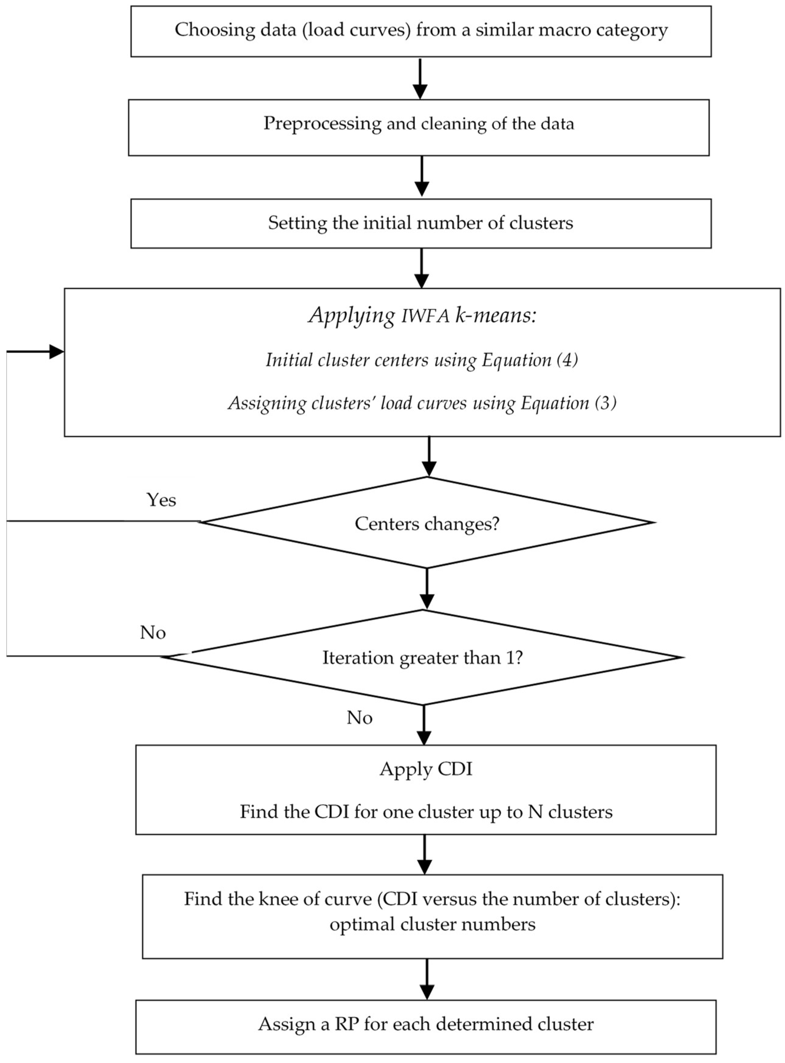
The overall clustering procedure based on the improved WFA k-means is illustrated in Figure 2.
2.2. Microgrid Pricing Scheme
Having obtained the RPs from clustering step, the microgrid can design its proper pricing schemes in step 2. To this end, the operator seeks to maximize its profit (or minimizes its cost). A comprehensive framework for this pricing scheme can be complicated, where the operator has to consider the energy that it buys from the upstream grid, which might be uncertain, and then sell it to consumers considering the proposed pricing scheme in this paper. This leads to a complex mathematical optimization, which is usually solved through a typical stochastic programming approach [9,22,23,24,25]. Please note that this comprehensive framework is not the focus of our current work, where our main aim is to develop clustering techniques to facilitate various pricing schemes and options for microgrid operators. Depending on the network conditions, peak demand, wholesale market prices, and the distributed energy resources which a microgrid has, it could decide on the optimal pricing schemes. The load curve clustering could alleviate to determine customer-targeted pricing schemes. For example, those customers having a similar pattern as the wholesale prices would be targeted for real-time pricing or other schemes such as ToU with high pricing during peak wholesale prices. In our future work, we intend to further develop this work to present a comprehensive model for microgrid energy scheduling.
3. Numerical Results
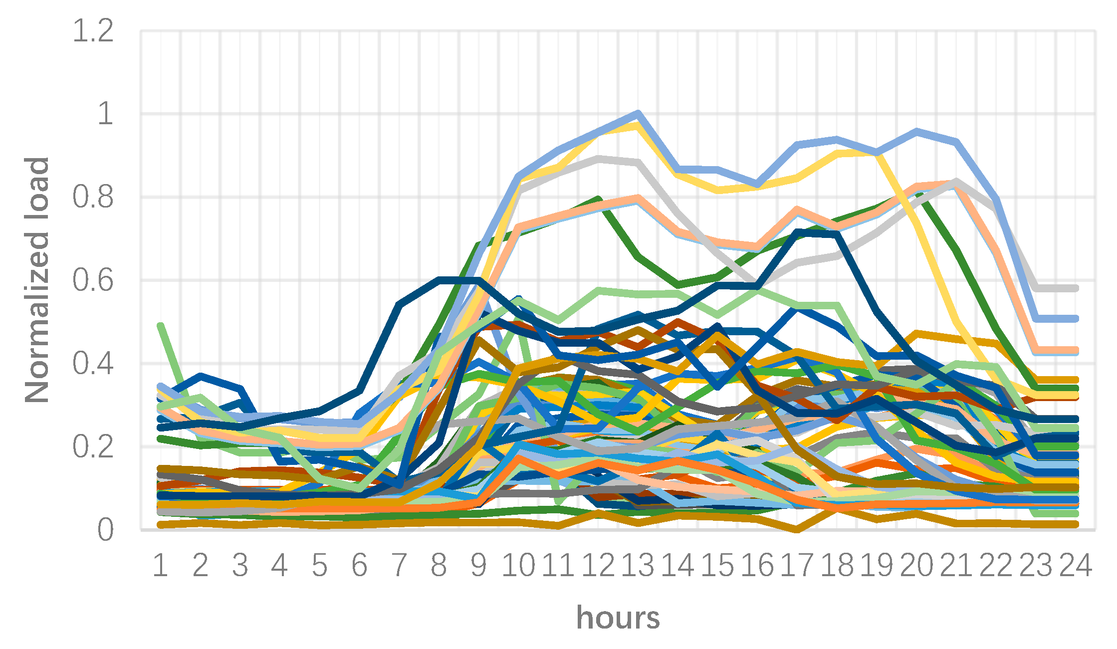
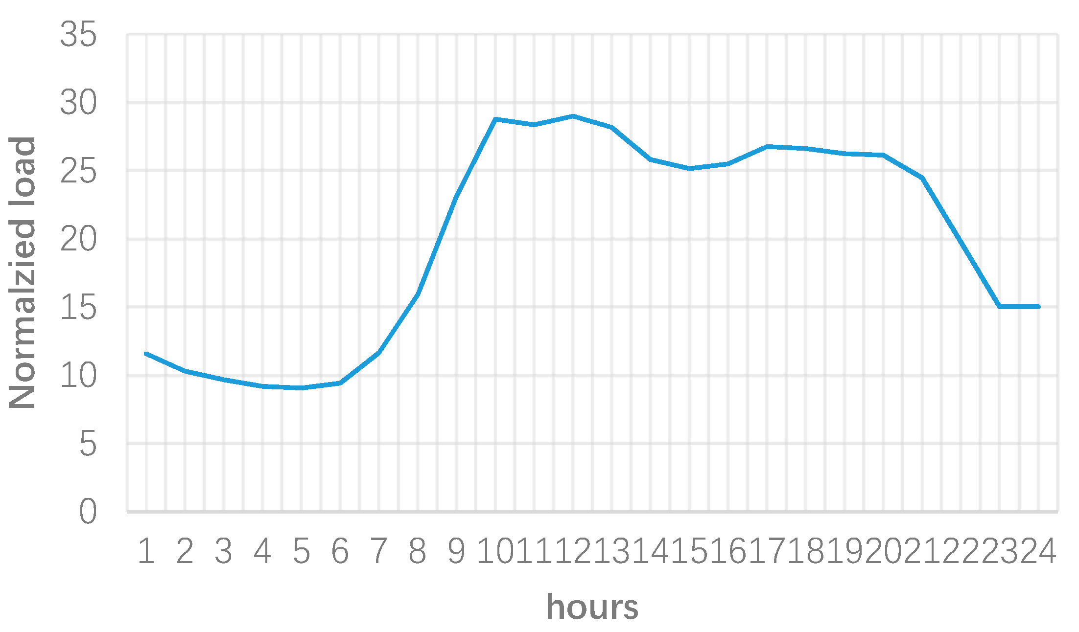
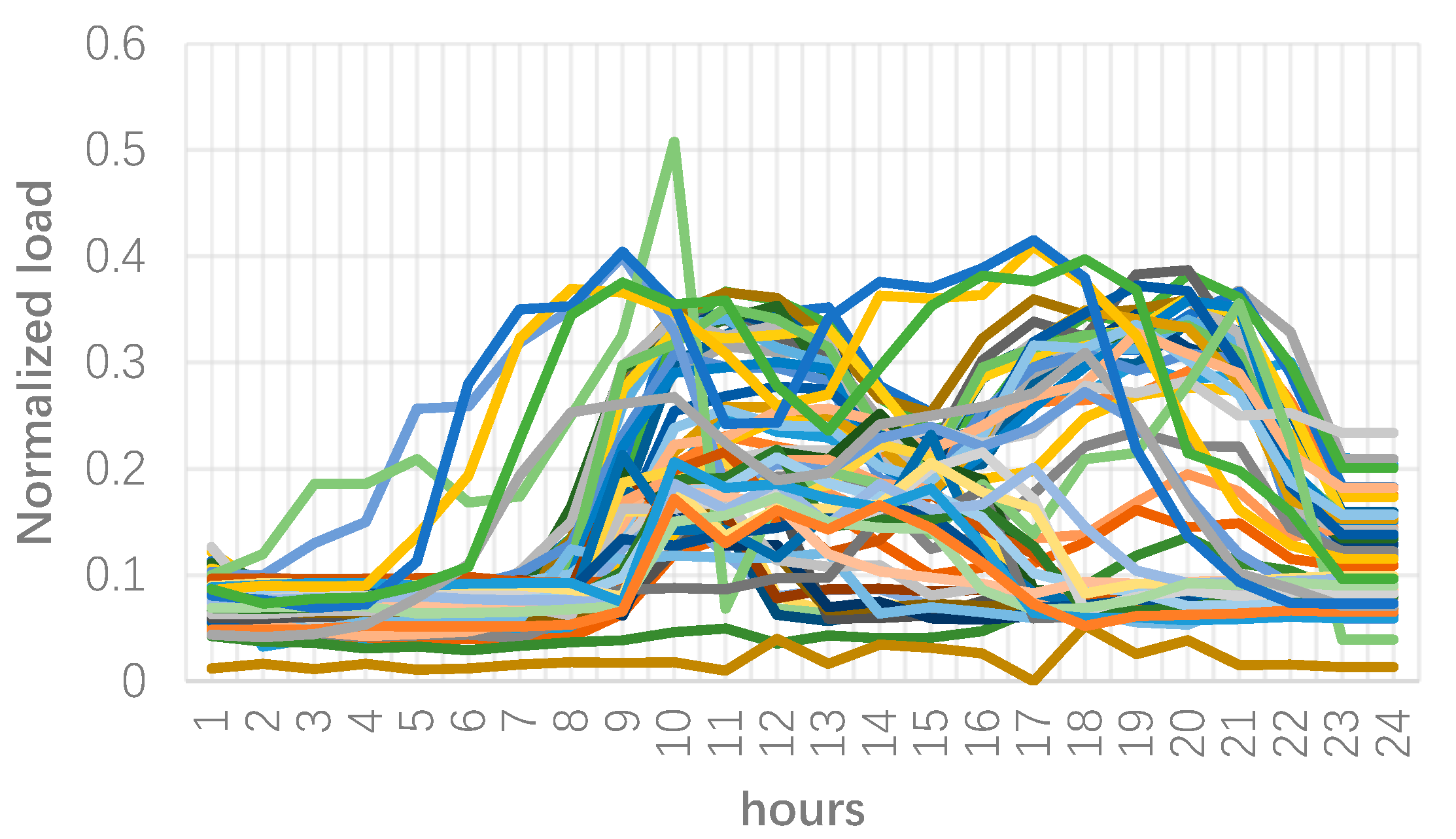
In order to implement the proposed approach, 75 customers in a distribution level are chosen. The data was provided by a Tehran distribution network service provider, but in an agreement for confidential feeders. Figure 3 shows the normalized load curve of these customers and Figure 4 represents the total curve of these profiles. As can be seen, various load curves exist which make determining a single price tariffs difficult and inefficient. Further, the total load illustrates that the customers impose a peak load around noon and another peak load in the evening. If the pricing is defined based on the load profile in Figure 4, the noon peak could be reduced but at the same time there could be risk of worsening evening peak. However, the following clustering results could bring an advantage to the microgrid to define smart pricing schemes.
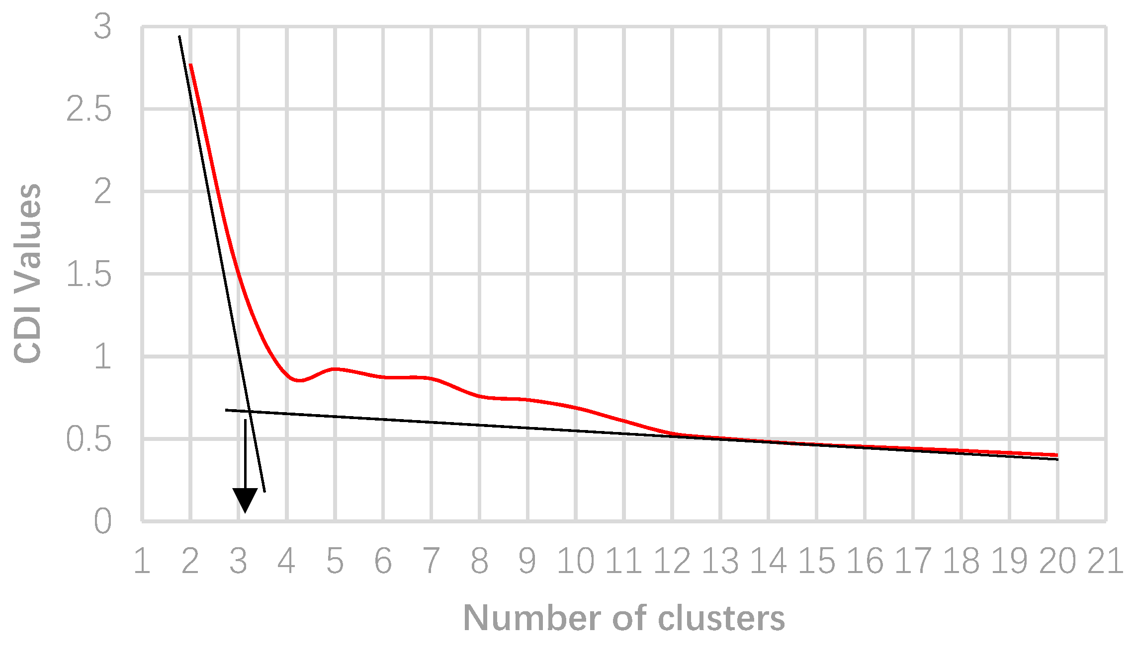
The improved WFA k-means is applied to the given load curves and a range of cluster numbers between 1 and 20 clusters are obtained. In order to determine the optimal number of clusters, the CDI measure is applied for each cluster number and its values are calculated. Then, the CDI values are plotted against the number of clusters, as given in Figure 5. As can be seen, the CDI values decrease as the number of clusters increases, which means the load profiles have more similarities in each cluster, but more dissimilarities compared with other clusters. As mentioned earlier, it is proven that the knee of this curve represents the optimal number of clusters. As such, according to Figure 5, this number is equal to three clusters.
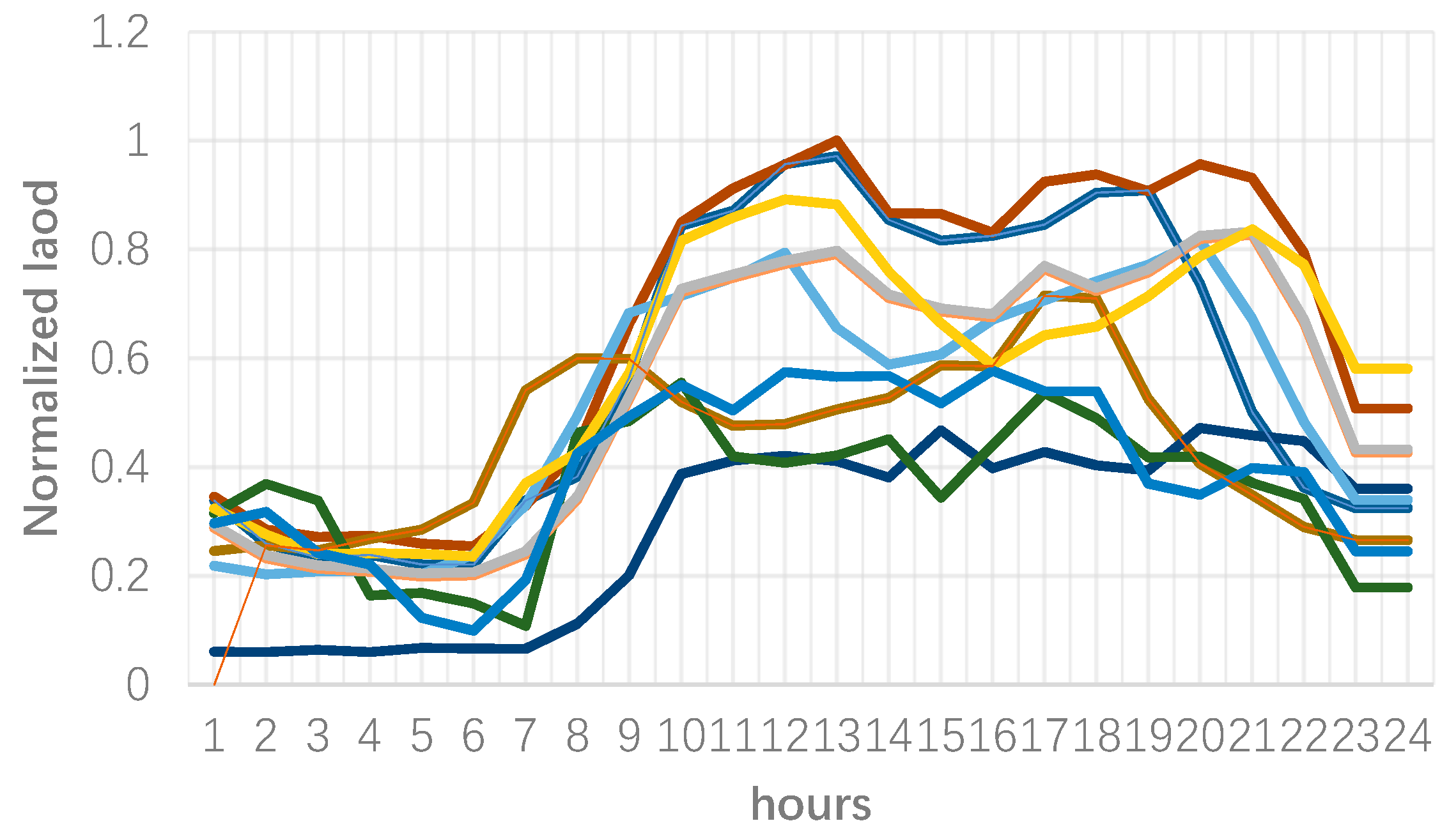
Having obtained the number of clusters, load curves in each cluster are identified. Sixty customers are clustered in class 1, while the number of load curves in clusters 2 and 3 are 5 and 10, respectively. Figure 6, Figure 7 and Figure 8 provide load curves in each cluster. As can be seen, cluster 1 accounts for those customers which have two peak periods around noon and in the evening. Further, their peak load is around 40% of the maximum load of all customers. Note that, these customers have a very short time of medium load between the two peak periods, while other periods have low load consumption.
Custer 2 involves those customers which have a peak load during the working hours. These customers are indeed some commercial customers which have low consumption. Their peak is indeed 50% of the maximum load of all customers.
Cluster 3 represents those customers with high consumption among all clusters. Further, it can be seen that these customers have a higher load around noon, while the second peak, which is lower than the noon peak load, happens in the evening.
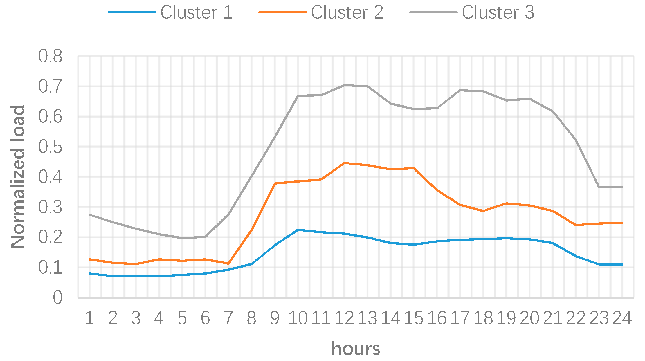
Having the load curves in each cluster, the center of each cluster can be determined. The center of each cluster provides the representative profile (RP) of the relevant cluster. Figure 9 delivers the RPs of the given clusters. The RPs indeed clearly confirm the discussion of load curves in each cluster, given in Figure 5, Figure 6, Figure 7 and Figure 8. Thus, the microgrid could target cluster 3 to reduce both their noon and evening peak load, whereas cluster 2 could be targeted for noon peak clipping.
Considering the representative profiles obtained through load clustering, the microgrid operator is now able to define proper pricing schemes. Following scenarios are some cases that the microgrid operator can consider.
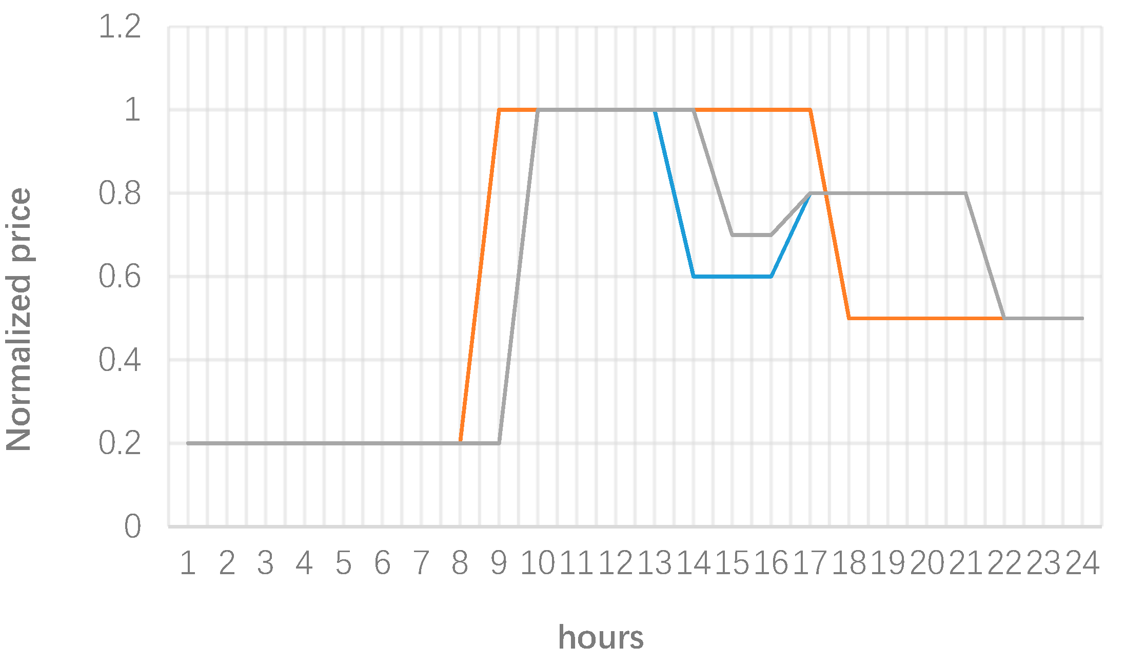
If the customers are inelastic, the microgrid can uses the RPs to determine optimal time of use tariffs. This allows the operator to achieve a higher revenue by charging consumers according to their representative load profile. As an example, Figure 10 provides the normalized time of use tariffs for each cluster. Note that the prices can be scaled up based on the actual prices that the microgrid operator determines based on its optimization procedure.
In case that all customers have smart meters with the ability of real-time pricing, this type of pricing scheme can be easily determined based on RPs. That is, considering real-time prices which have similar patterns to the RPs of each cluster will help the operator to increase its revenue of selling energy to consumers. To this end, the real-time price patterns can exactly follow the RPs in Figure 9.
If some consumers are elastic to prices, they may reduce their load during peak prices. This load can be shifted to off-peak periods or even curtailed without recovery in off-peak periods. The load shifting program is dependent on the elasticity of consumers. This program is defined as follows.
where, is the initial demand of consumers before demand response. is the demand after conducting the demand response program. is the initial price of consumers before demand response. is the new pricing model for load reduction programs. The elasticity of consumers between the i-th and j-th hours is defined as:
Note that cross elasticity is defined as the elasticity of consumers to the price in other periods, while self-elasticity is the sensitivity of consumers to the price in the relevant period.
By carrying out the given program, and depending on the consumers’ elasticity, the microgrid operator can shift the load from peak hours, particularly around noon which coincides the system peak as shown in Figure 4, to off-peak periods, e.g., early morning. However, this program requires a deep understanding of the characteristics of consumers. Although detailed studies are required for this purpose, one key solution is using the RPs derived from load clustering in step 1, i.e., Figure 9. Considering this figure, the following findings for the given demand response programs can be interpreted. First, consumers in cluster 1 are the most suitable customers for implementing the given demand response program. This is due to the following reasons. As can be seen from Figure 9, these consumers have the highest consumption among all clusters. As such, it would be easier to achieve the targeted load reduction during peak hours if these consumers are considered as the priority. Second, these consumers are high consuming residential customers which their peak consumption coincides with the system peak. Therefore, these consumers might be in a category that has family members staying at home during the day, and using their electric appliances in this period, which indicate the high possibility of achieving load reduction from them. Cluster 2 has the lowest load reduction capability due to following reasons. First, these consumers are more likely small to medium commercial customers, which have low ability to shift their load to other periods. Further, their consumption compared to cluster 1 is low, which shows lower priority for these consumers to carry out demand response. Lastly, cluster 3 has also low demand response potential. Although their peak load coincides the system peak load, these consumers peak is less than 20% of the maximum load of all consumers. That is, these consumers are expected to have the low share of shift-able loads compared to consumers in cluster 3. As a result, it can be highlighted that the proposed approach helps microgrid operators better identify the consumers having demand response potential. First, this approach helps classify consumers and then identifying their features such as their type (residential, commercial, etc.), their consumption level (high, low, medium), their coincidental peak load with the system peak, and other relevant features. Moreover, identifying proper consumers from a large number of consumers for suitable demand response programs is not a practical approach. Thus, deploying clustering techniques to group these consumers in a reasonable number of classes would facilitate this for the microgrid operator.
4. Conclusions
This paper presents a new model for pricing by microgrid operators in which the operator uses clustering techniques to classify consumers load curves into a specific number if clusters, which help identify their representative profiles (RPs) and also reduce the size of data on which the operator has to work. Having this RPs, the operator can identify the consumers’ type in each cluster, and other features such as their consumption level and whether their peak load coincides the system peak. This helps the operator to decide best pricing schemes such as real-time pricing and time of use tariffs for consumers, as well as to define possible demand response and load reduction programs for consumers to reduce its system peak load.
The proposed model is applied on 75 load curves of consumers and the results are obtained. Optimal numbers of clusters are defined, which shows distinctive consumers in three clusters. Each cluster’s RP represents its consumers’ characteristics. While clusters 1 and 3 include residential consumers with high and low consumption, respectively, cluster 2 includes low energy consuming commercial consumers. Considering these RPs’ various pricing models and typical time of use tariffs are suggested. Further, the clusters are prioritized for demand response actions to reduce the peak load of the microgrid during the noon.
This work can be extended to consider a comprehensive model which takes into account energy purchasing from the wholesale market and then selling it through the defined pricing scheme to consumers by the microgrid operator.
Author Contributions
Conceptualization, H.L. and N.M.; Methodology, H.L. and N.M.; Validation, H.L. and N.M.; Formal Analysis, H.L. and N.M.; Data Curation, K.C.; Writing-Original Draft Preparation, H.L., N.M. and K.C.; Writing-Review & Editing, H.L.
Acknowledgments
Jiangsu Province Laboratory of Mining Electric and Automation gives the support of working places and experiment places. The paper is Nadali’s work, not Ernst & Young view.
Conflicts of Interest
The authors declare no conflict of interest.
Nomenclatures
| The hth component of weighted fuzzy average in the rth iteration | |
| Variance of WFA k-means | |
| Variance of the hth component of load profiles | |
| Average variance | |
| Adjusting parameter | |
| Adjusting parameter | |
| The pth input curve | |
| The hth component of pth input curve | |
| Centeriod of the kth cluster | |
| The hth component of centeriod of the kth cluster | |
| The hth component of initial centeriod of the kth cluster | |
| The hth component of computed weight of the pth curve in the rth iteration |
References
- Yu, J.; Ni, M.; Jiao, Y.; Wang, X. Plug-in and plug-out dispatch optimization in microgrid clusters based on flexible communication. J. Mod. Power Syst. Clean Energy 2016, 5, 663–670. [Google Scholar] [CrossRef]
- Lo Prete, C.; Hobbs, B.F.; Norman, C.S.; Cano-Andrade, S.; Fuentes, A.; von Spakovsky, M.R.; Mili, L. Sustainability and reliability assessment of microgrids in a regional electricity market. Energy 2012, 41, 192–202. [Google Scholar] [CrossRef]
- Satapathy, P.; Dhar, S.; Dash, P.K. Stability improvement of PV-BESS diesel generator-based microgrid with a new modified harmony search-based hybrid firefly algorithm. IET Renew. Power Gener. 2017, 11, 566–577. [Google Scholar] [CrossRef]
- Li, Y.; Peng, Z.; Lingyu, R.; Orekan, T. A Geršgorin theory for robust microgrid stability analysis. In Proceedings of the 2016 IEEE Power and Energy Society General Meeting (PESGM), Boston, MA, USA, 17–21 July 2016; pp. 1–5. [Google Scholar]
- Xu, X.; Wang, T.; Mu, L.; Mitra, J. Predictive Analysis of Microgrid Reliability Using a Probabilistic Model of Protection System Operation. IEEE Trans. Power Syst. 2017, 32, 3176–3184. [Google Scholar] [CrossRef]
- Wang, S.; Zhang, X.; Ge, L.; Wu, L. 2-D Wind Speed Statistical Model for Reliability Assessment of Microgrid. IEEE Trans. Sustain. Energy 2016, 7, 1159–1169. [Google Scholar] [CrossRef]
- Guo, Y.; Xiong, J.; Xu, S.; Su, W. Two-Stage Economic Operation of Microgrid-Like Electric Vehicle Parking Deck. IEEE Trans. Smart Grid 2016, 7, 1703–1712. [Google Scholar] [CrossRef]
- Nguyen, D.T.; Le, L.B. Risk-Constrained Profit Maximization for Microgrid Aggregators with Demand Response. IEEE Trans. Smart Grid 2015, 6, 135–146. [Google Scholar] [CrossRef]
- Honarmand, M.; Zakariazadeh, A.; Jadid, S. Integrated scheduling of renewable generation and electric vehicles parking lot in a smart microgrid. Energy Convers. Manag. 2014, 86, 745–755. [Google Scholar] [CrossRef]
- Wu, T.; Yang, Q.; Bao, Z.; Yan, W. Coordinated Energy Dispatching in Microgrid with Wind Power Generation and Plug-in Electric Vehicles. IEEE Trans. Smart Grid 2013, 4, 1453–1463. [Google Scholar] [CrossRef]
- Hong, Y.-Y.; Chang, W.-C.; Chang, Y.-R.; Lee, Y.-D.; Ouyang, D.-C. Optimal sizing of renewable energy generations in a community microgrid using Markov model. Energy 2017, 135, 68–74. [Google Scholar] [CrossRef]
- Jin, M.; Feng, W.; Marnay, C.; Spanos, C. Microgrid to enable optimal distributed energy retail and end-user demand response. Appl. Energy 2017, 210, 1321–1335. [Google Scholar] [CrossRef]
- Liu, G.; Starke, M.; Xiao, B.; Zhang, X.; Tomsovic, K. Microgrid optimal scheduling with chance-constrained islanding capability. Electr. Power Syst. Res. 2017, 145, 197–206. [Google Scholar] [CrossRef]
- Colley, D.; Mahmoudi, N.; Eghbal, D.; Saha, T.K. Queensland load profiling by using clustering techniques. In Proceedings of the 2014 Australasian Universities Power Engineering Conference (AUPEC), Perth, Australia, 28 September–1 October 2014; pp. 1–6. [Google Scholar]
- Tiefeng, Z.; Guangquan, Z.; Jie, L.; Xiaopu, F.; Wanchun, Y. A New Index and Classification Approach for Load Pattern Analysis of Large Electricity Customers. IEEE Trans. Power Syst. 2012, 27, 153–160. [Google Scholar]
- Tsekouras, G.J.; Kotoulas, P.B.; Tsirekis, C.D.; Dialynas, E.N.; Hatziargyriou, N.D. A pattern recognition methodology for evaluation of load profiles and typical days of large electricity customers. Electr. Power Syst. Res. 2008, 78, 1494–1510. [Google Scholar] [CrossRef]
- Kohan, N.M.; Moghaddam, M.; Bidaki, S.; Yousefi, G. Comparison of modified k-means and hierarchical algorithms in customers load curves clustering for designing suitable tariffs in electricity market. In Proceedings of the 43rd International Universities Power Engineering Conference, Padova, Italy, 1–4 September 2008; pp. 1–5. [Google Scholar]
- Wenyuan, L.; Jiaqi, Z.; Xiaofu, X.; Jiping, L. A Statistic-Fuzzy Technique for Clustering Load Curves. IEEE Trans. Power Syst. 2007, 22, 890–891. [Google Scholar]
- Mahmoudi-Kohan, N.; Eghbal, M.; Moghaddam, M. Customer recognition-based demand response implementation by an electricity retailer. In Proceedings of the 2011 21st Australasian Universities Power Engineering Conference (AUPEC), Brisbane, Australia, 25–28 September 2011; pp. 1–6. [Google Scholar]
- Chicco, G.; Napoli, R.; Piglione, F. Comparisons among clustering techniques for electricity customer classification. IEEE Trans. Power Syst. 2006, 21, 933–940. [Google Scholar] [CrossRef]
- Mahmoudi, N.; Saha, T.K.; Eghbal, M. Wind offering strategy in the Australian National Electricity Market: A two-step plan considering demand response. Electr. Power Syst. Res. 2015, 119, 187–198. [Google Scholar] [CrossRef]
- Mahmoudi, N.; Saha, T.K.; Eghbal, M. A new demand response scheme for electricity retailers. Electr. Power Syst. Res. 2014, 108, 144–152. [Google Scholar] [CrossRef]
- Amini, M.H.; Kargarian, A.; Karabasoglu, O. ARIMA-based decoupled time series forecasting of electric vehicle charging demand for stochastic power system operation. Electr. Power Syst. Res. 2016, 140, 378–390. [Google Scholar] [CrossRef]
- Mahmoudi, N.; Eghbal, M.; Saha, T.K. Employing demand response in energy procurement plans of electricity retailers. Int. J. Electr. Power Energy Syst. 2014, 63, 455–460. [Google Scholar] [CrossRef]
- Eghbal, M.; Saha, T.K.; Mahmoudi-Kohan, N. Utilizing demand response programs in day ahead generation scheduling for micro-grids with renewable sources. In Proceedings of the Innovative Smart Grid Technologies Asia (ISGT), Perth, Australia, 13–16 November 2011; pp. 1–6. [Google Scholar]
Figure 1.
The proposed two-step pricing scheme.

Figure 2.
The procedure of the proposed improved WFA k-means.

Figure 3.
Load curve of all consumers.

Figure 4.
Total load curve of all consumers.

Figure 5.
CDI versus the number of clusters.

Figure 6.
Load curves of consumers in cluster 1.

Figure 7.
Load curves of consumers in cluster 2.

Figure 8.
Load curves of consumers in cluster 3.

Figure 9.
Representative Patterns (RPs) of all clusters.

Figure 10.
A typical time of use tariff for each cluster.

© 2018 by the authors. Licensee MDPI, Basel, Switzerland. This article is an open access article distributed under the terms and conditions of the Creative Commons Attribution (CC BY) license (http://creativecommons.org/licenses/by/4.0/).
Share and Cite
MDPI and ACS Style
Liu, H.; Mahmoudi, N.; Chen, K. Microgrids Real-Time Pricing Based on Clustering Techniques. Energies 2018, 11, 1388. https://doi.org/10.3390/en11061388
AMA Style
Liu H, Mahmoudi N, Chen K. Microgrids Real-Time Pricing Based on Clustering Techniques. Energies. 2018; 11(6):1388. https://doi.org/10.3390/en11061388
Chicago/Turabian StyleLiu, Hao, Nadali Mahmoudi, and Kui Chen. 2018. "Microgrids Real-Time Pricing Based on Clustering Techniques" Energies 11, no. 6: 1388. https://doi.org/10.3390/en11061388
Note that from the first issue of 2016, this journal uses article numbers instead of page numbers. See further details here.