Pressure Detrending in Harmonic Pulse Test Interpretation: When, Why and How

Abstract

In reservoir engineering, one of the main sources of information for the characterization of reservoir and well parameters is well testing. An alternative to the standard drawdown/buildup test is Harmonic Pulse Testing (HPT) because it can provide well performance and reservoir behavior monitoring without having to interrupt field production, which is appealing from an economic standpoint. Recorded pressure analysis is performed in the frequency domain by adopting a derivative approach similar to conventional well testing. To this end, pressure and rate data must be decomposed into harmonic components. Test interpretability can be significantly improved if pressure data are detrended prior to interpretation, filtering out non periodic events such as discontinuous production from neighboring wells and flow regime variations that did not respect the designed test periodicity. Therefore, detrending offers the possibility of overcoming the limitation of HPT applicability due to the difficulty of imposing a regularly pulsing rate for the whole test duration (typically lasting several days). This makes HPT attractive for well performance monitoring, especially in gas reservoirs converted to underground gas storage. In this paper, different detrending methodologies are discussed and applied to synthetic and real data. Results show that, if a proper detrending strategy is adopted, information provided by HPT interpretation can be maximized and/or improved.

1. Introduction

Well testing provides pressure measurements that are mainly used for determining reservoir-rock properties and boundaries of the producing formation; as such, it is considered an effective method of reservoir analysis. Conventional well tests have been used by reservoir engineers to evaluate well and reservoir performance for decades [1,2,3,4,5]. Over the last several years, research has focused on developing complementary well test methodologies that are both less expensive and more environmentally friendly procedures [6,7,8,9,10,11,12,13,14]. These well test methodologies were designed to provide essential information (i.e., kh and skin) when standard well testing procedure cannot be applied. Among the complementary well testing methodologies, Harmonic Pulse Testing (HPT) is appealing from an economic standpoint as it can provide well performance and reservoir monitoring without having to interrupt field production. In HPT, a pulsed signal is superimposed onto the background pressure trend; thus, no interruption of well and reservoir production is required before and during the test.

Simple Pulse testing as a methodology for reservoir properties characterization dates back to 1966 when it was first proposed by Johnson et al. [15]. Since then, theoretical developments have led to the current characteristic of periodicity of the original test procedure, which allows the application of interpretation methodology in the frequency domain [16,17,18,19,20,21,22,23,24,25,26,27,28,29,30,31,32,33]. Thus, a harmonic test is that in which the injection or production rate is varied in a periodic way. These rates can be imposed after a long shut in of the tested well, like in conventional well testing, or they can be superposed to ongoing production without interruption of production activities from other wells, hence the economic benefit of the methodology. However, HPT does show a limitation in terms of the investigation distance, which is shorter for the same test duration as compared to that of a conventional well test. Additionally, reliable test interpretation means regular sampling of the pressure data and reasonable periodicity of the imposed rate signal. Despite the aforementioned, HPT methodology and interpretation does not require the initial static pressure nor the previous production history of the well, which in turn are considerable advantages [33].

Pressure and rate signals recorded during HPT are first analyzed in the frequency domain with proper methodologies, mainly based on Fourier Analysis, to then be interpreted by adopting a derivative approach similar to that of a conventional well test [33]. Pressure data should be adequately pre-processed with detrending methodologies to separate pure periodic components of the signal from non-periodic components; in this way, the information obtained from HPT interpretation can be maximized. First transient magnitude, discontinuous production from neighboring wells, and flow regime variations produce a significant non-periodic component in the pressure response that might strongly affect the periodicity of the pressure signal and hence the reliability of test interpretation.

To filter out non-periodic components, different detrending approaches have been suggested in the literature: for instance, Hollaender [20] adopted a polynomial reconstruction of the aperiodic depletion trend; and, more recently, detrending approaches based on a heuristic reconstruction of a constant depletion have been presented [25,34].

In the present paper, four detrending methodologies (method 0, method 1, method 2 and method 3 hereinafter) are considered and discussed. Method 0 is the simple linear detrending. Method 1 is an interesting and efficient heuristic algorithm proposed by Ahn and Horne [25]. Methods 2 and 3 [34] are heuristic algorithms developed in steps by the authors, initially with the aim of overcoming some limitations of the Ahn and Horne algorithm [25], and subsequently to extend the approach to any possible scenario as well as to better characterize the periodic and the non-periodic components.

The four detrending algorithms were applied to several synthetic cases representative of possible scenarios and to a real gas storage case. The resulting detrended harmonic signals were analyzed in the frequency domain adopting the approach presented by Fokker et al. [33] and compared in terms of quality of the harmonic components derivative and interpretation results. Furthermore, the four detrending algorithms were applied to a real case in which temporary test interruptions due to operational constraints negatively affected pressure response periodicity.

2. Detrending Methodologies

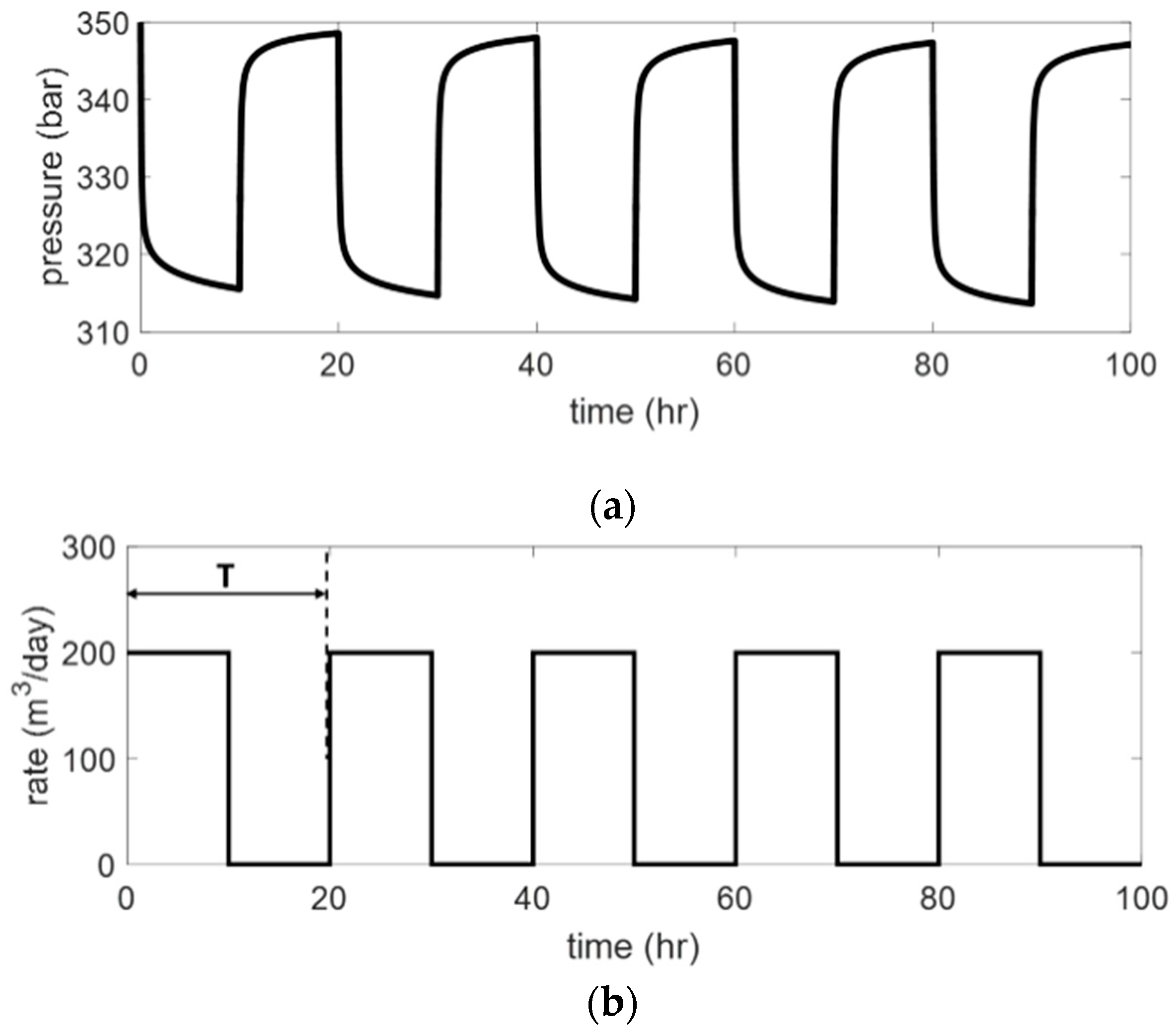
Detrending refers to methodologies aimed at removing from a time series any trend that can mask or affect the information of interest. In the case of HPT, detrending refers to recognizing a non-periodic depletion trend and removing it from the pressure signal to isolate the pure periodic component. The four detrending methodologies discussed in this paper do not require any model or parameter characterization. They are based on the observation of the pressure data only (methods 0 and 1), or on the observation of the pressure and rate data (methods 2 and 3), and they try to approximate or reconstruct the non-periodic component of the pressure signal.

Consider a harmonic squared rate production history as shown in Figure 1 and the corresponding pressure response. T is the period of the harmonic signal. According to the terminology adopted in the oil industry for well testing, T/2 corresponds to the duration of each flow period. The rates adopted to impose the harmonic oscillation will be indicated as q₁ and q₂, whereas q₀ refers to the last historical rate preliminary to the HPT. In the adopted nomenclature, n_T is the total number of periods T. If q₀ is null, initial static conditions are assumed at the beginning of the test; furthermore, q₂ = 0 implies that the HPT is defined as a sequence of Draw Down (DD with q₁ > 0) and Build Up (BU q₂ = 0). Therefore, the initial transient state magnitude associated with the first flow period is comparable to the transient state magnitude associated with the following DDs. Whenever q₀ is null but neither q₁ nor q₂ are null, the harmonic pressure oscillation is influenced by an initial transient characterized by an amplitude higher with respect to the subsequent oscillations. The magnitude of the initial transient affects mainly the first DD and progressively attenuates during the test. When the HPT is superimposed onto ongoing production (i.e., q₀ ≠ 0, no well shut in before the test is imposed), the magnitude of the initial transient is proportional to the difference between the previous rate before the test (q₀) and the second test rate (q₂). In the following paragraphs, it is assumed that q₁ > q₂ and therefore q₁ is named q_max and q₂ is named q_min. Furthermore, it is assumed that q_max > q₀.

2.1. Method 0: Linear Detrending

Linear detrending is an adequate strategy in scenarios dominated by depletion, either due to late time effects (boundaries) or to field activities; however, it is not able to filter the initial transient due to the difference between the last rate preceding the test (q₀) and the rate of the second hemicycle of oscillation (q_min). In the analyzed scenarios, the linear trend parameters (slope and known term) are obtained by least square fitting of pressure data.

2.2. Method 1: Ahn and Horne Approach

The methodology proposed by Ahn and Horne [25] is based on pressure data only and does not require information on petrophysical properties and fluid parameters. The algorithm was designed to detrend HPT pressure signals similar to the example in Figure 1, therefore assuming both q₀ and q_min are equal to zero. The approach suggested by Ahn and Horne consists in generating an approximation of the constant rate pressure trend $g\left(t\right)$ at each time $t_n=\frac{2n+1}{2}T$ for n = 1, …, n_T − 1 and linearly interpolating $g\left(t\right)$ between each couple of points t_n−1, t_n. The algorithm is:

$$g(t_n)=h(t_n)+h\left(t_n-\frac{T}{2}\right),$$

(1)

where $h(t_n)$ and $g(t_n)$ denote the observed periodic pulse and the constant rate approximation, respectively, at a time t_n.

The suggested approach does not require any information on the value of the rate produced during the Draw Down periods, but this implies that the production history is assumed to be an alternation of production/injection periods (Draw Down or Injection) and well shut in (Build Up or Fall Off). Consequently, it was not designed to detrend a pressure signal generated for $q_{min}\ne q_0$ when the amplitude of the first transient can be significant, especially if $\left|q_{max}-q_0\right|\gg \left|q_{max}-q_{min}\right|$. However, in scenarios where $\left|q_{max}-q_0\right|\approx \left|q_{max}-q_{min}\right|,$ detrending is not strictly necessary unless significant reservoir depletion, due to production from other wells, is observed.

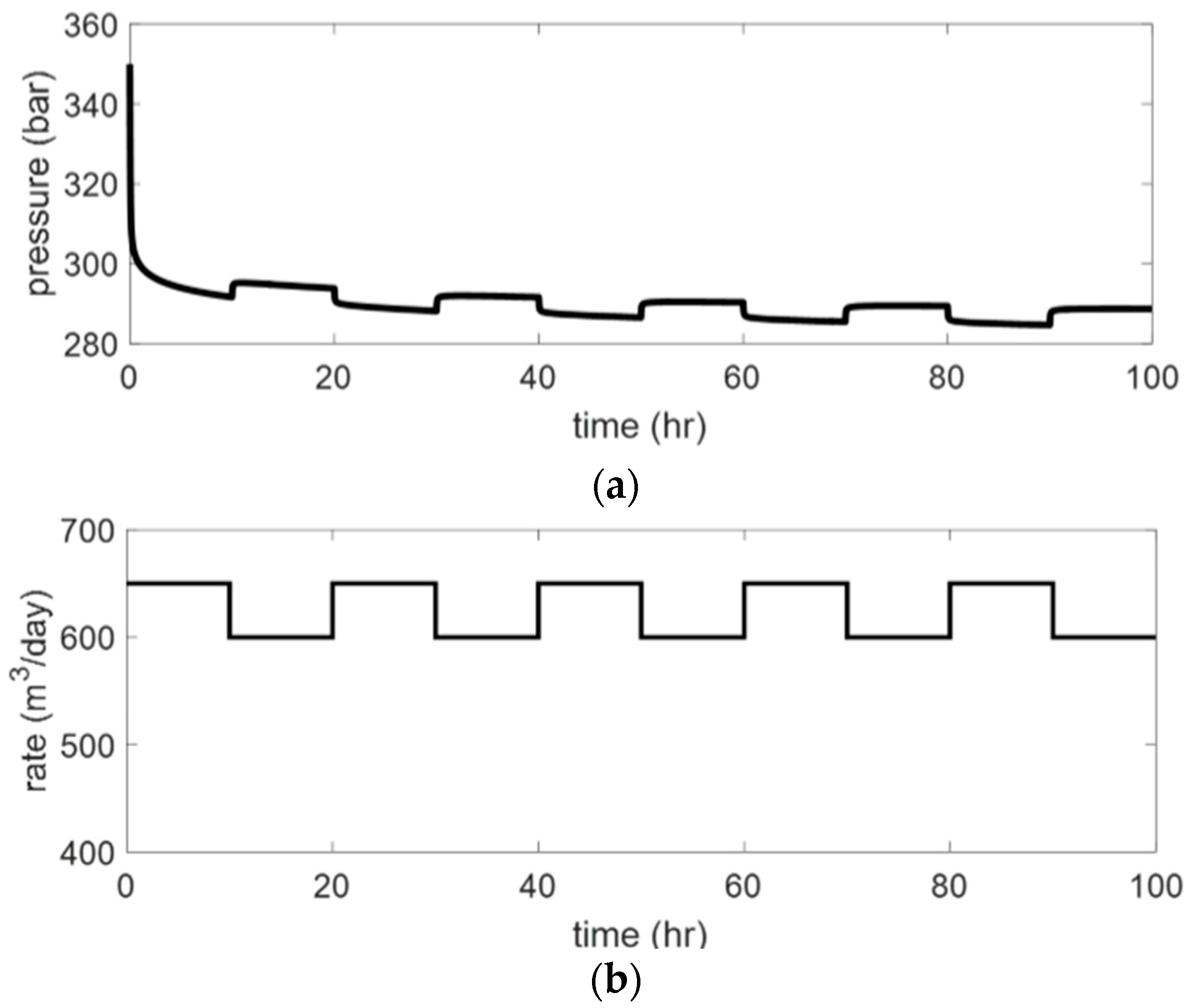
2.3. Method 2: Rate Generalized Approach with Stepwise Linear Interpolation

A new algorithm that provides an extension to the approach proposed by Ahn and Horne for any possible combination of q_min and q_max was derived by the authors. The algorithm represents the first step of the approach proposed by Viberti [34] and was obtained analytically by applying the superposition principle. Consider the pressure signal associated with an HPT characterized by q_min different from 0 and the maximum rate significantly higher with respect to the rate variation (see Figure 2). The goal of the algorithm consists of calculating the reconstructed pressure signal corresponding to a constant rate equal to q_max for a time vector containing the elements $t_n=\frac{1}{2}T, T,\frac{3}{2}T,2T,\dots ,n_{T}T$.

In order to take into account the first transient due to the condition $\left|q_{max}-q_0\right|\gg \left|∆q\right|$, where $∆q=q_{max}-q_{min}$, a normalized periodic rate variation is defined as:

$$\tilde{q}=\frac{∆q}{q_{max}}.$$

(2)

Adopting $g\left(t\right)$ and $h\left(t\right)$ as for the Ahn and Horne approach, and considering, as a simplified example, an HPT characterized by a n_T = 2, it is possible to write a system of linear equations so that:

$$\{\begin{array}{l}h\left(\frac{1}{2}T\right)=q_{max} g\left(\frac{1}{2}T\right),\hfill \\ h\left(T\right)=q_{max} g\left(T\right)-∆qg\left(\frac{1}{2}T\right),\hfill \\ h\left(\frac{3}{2}T\right)=q_{max} g\left(\frac{3}{2}T\right)-∆qg\left(T\right)+∆qg\left(\frac{1}{2}T\right),\hfill \\ h\left(2T\right)=q_{max} g\left(2T\right)-∆qg\left(\frac{3}{2}T\right)+∆qg\left(T\right)-∆qg\left(\frac{1}{2}T\right).\hfill \end{array}$$

(3)

The system of equations was obtained by the application of the superposition principle imposing a sequence of positive and negative rate variations.

The system of linear equations can be easily written as in Equation (4) and solved through matrix inversion in order to find all the $g\left(i\frac{T}{2}\right)$ with i = 1, …, 2n_T:

$$\left[\begin{array}{c}\begin{array}{c}h\left(\frac{1}{2}T\right)\\ h\left(T\right)\\ h\left(\frac{3}{2}T\right)\end{array}\\ h\left(2T\right)\end{array}\right]=∆q\left[\begin{array}{cccc}\raisebox{1ex}{$1$}\!\left/ \!\raisebox{-1ex}{$\tilde{q}$}\right.& 0& 0& 0\\ -1& \raisebox{1ex}{$1$}\!\left/ \!\raisebox{-1ex}{$\tilde{q}$}\right.& 0& 0\\ 1& -1& \raisebox{1ex}{$1$}\!\left/ \!\raisebox{-1ex}{$\tilde{q}$}\right.& 0\\ -1& 1& -1& \raisebox{1ex}{$1$}\!\left/ \!\raisebox{-1ex}{$\tilde{q}$}\right.\end{array}\right]\left[\begin{array}{c}\begin{array}{c}g\left(\frac{1}{2}T\right)\\ g\left(T\right)\\ g\left(\frac{3}{2}T\right)\end{array}\\ g\left(2T\right)\end{array}\right].$$

(4)

An approximation of the constant rate pressure signal is then obtained through linear interpolation between any couple of values $g\left(i\frac{T}{2}\right)$ and $g\left(\left(i-1\right)\frac{T}{2}\right)$.

2.4. Method 3: Rate Generalized Approach with Full Heuristic Reconstruction

Method 3 overcomes the simplified assumption of linear interpolation adopted by method 2 and provides a heuristic reconstruction of the constant rate pressure signal for all the elements of the original time and pressure vectors for any periodic rate history and therefore also for $\left|q_{max}\right|\gg \left|q_{max}-q_{min}\right|$. The algorithm derivation and details have already been published [34] and are briefly summarized here. The algorithm is based on the application of the superposition principle for the identification of recurring events (therefore characterized by periodicity) from a sequence of observations. As a consequence, it is based on the analysis of all the semi-periods of a periodic signal at the same $∆t$ in all the intervals $i\frac{T}{2}\le ∆t<\left(i+1\right)\frac{T}{2}$. To do so, a dimensionless time variable $\chi \in ℝ$ is defined so that $t=\chi \frac{T}{2}$, therefore $\chi \in \left[0,2n_T\right]$.

The observations and the sought constant rate response can be written as $h\left(\chi ,T\right)$ and g$\left(\chi ,T\right)$, respectively, and, adopting the definition of $\tilde{q}$ introduced for method 2, observation at each recurrent $∆t$ can be expressed as $h\left(\left(\chi -j\right)\frac{T}{2}\right)$ writing a system of $2n_T$ equations with $j=0,\dots , 2n_T-1$, so that:

$$h\left(\left(\chi -j\right)\frac{T}{2}\right)=∆q\frac{1}{\tilde{q}}g\left(\left(\chi -j\right)\frac{T}{2}\right)+∆q{\displaystyle \sum }_{i=j+1}^{2n_T-j-1}-1^{i}g\left(\left(\chi -i\right)\frac{T}{2}\right), j=0,\dots ,2n_T-1.$$

(5)

The obtained system of linear equations can then be easily solved. The resulting constant rate pressure signal is multiplied by a proper rate value and subtracted to the original pressure signal in order to obtain the detrended harmonic pressure component.

3. Results

In order to validate and compare the presented detrending methodologies, several synthetic cases were generated. Each case represents a different scenario characterized by both reservoir behavior and production operations or events that can potentially affect the test. From a reservoir behavior viewpoint, three main scenarios were considered: simple homogeneous system, presence of one boundary within the investigated area of the test, and a closed system with high depletion. From a production operations or events viewpoint, several possible situations were taken into account: interfering well produced with constant rate, interfering well production with rate variation longer than the oscillation period, interfering well production with rate variation shorter than the oscillation period, well shut in prior to test, and complex historical production preceding the test. In all scenarios, the use of a detrending algorithm proved valuable to improve data quality and hence test interpretation. A selection of the scenarios is described in detail in the following Section 3.1, Section 3.2, Section 3.3 and Section 3.4 of this paper. The common data adopted for the generation of synthetic cases are summarized in

Table 1. Reservoir and well parameters adopted for synthetic case generation.

Parameters	Values
Permeability	100 mD
Porosity	0.2
Net pay	10 m
Initial pressure	300 105 Pa
Total compressibility	1.646 10−9 Pa−1
Oil volume factor	1.3
Oil viscosity	1 cP
Well radius	0.1 m
Wellbore storage	1 10−8 Pa/m
Skin	0

; pressure and rate data are generated with a constant sampling interval of 10 s. The rates adopted to impose the harmonic oscillation will be indicated as q₁ and q₂, whereas q₀ refers to the last historical rate prior to the HPT. The rate is obviously null when initial static conditions are simulated at the beginning of the test. In addition, a real gas well HPT was analyzed; the test was interrupted twice for several hours because of operational constraints, thus inducing two considerable irregularities in the pressure periodical trend.

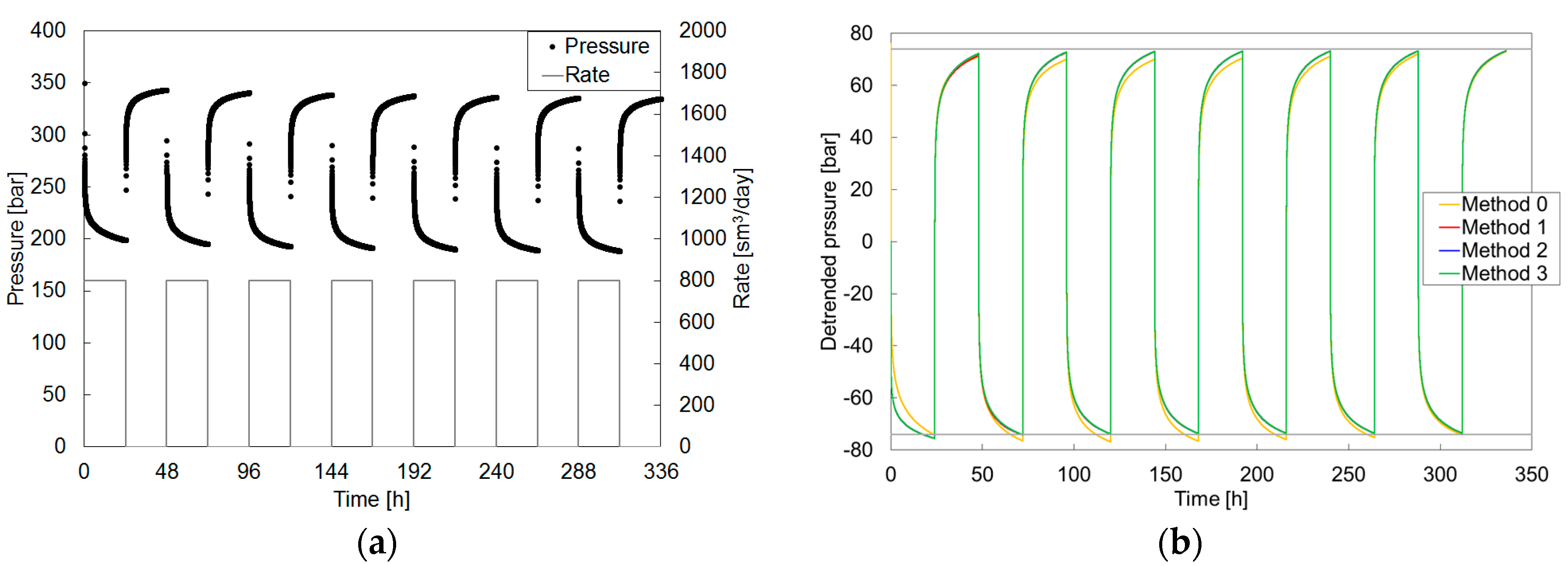
3.1. Synthetic Case 1: Ideal Condition

The first selected case presents ideal conditions to preserve the periodic trend of pressure response. Production starts from the initial static conditions. The test consists of seven oscillating cycles in which constant production of q₁ = 800 m³/day is alternated with shut in of q₂ = 0 m³/day every 24 h (Figure 3a). Neither well interference nor significant overall pressure decline are imposed. Moreover, the influence of the initial transient is very limited because q₂ = q₀.

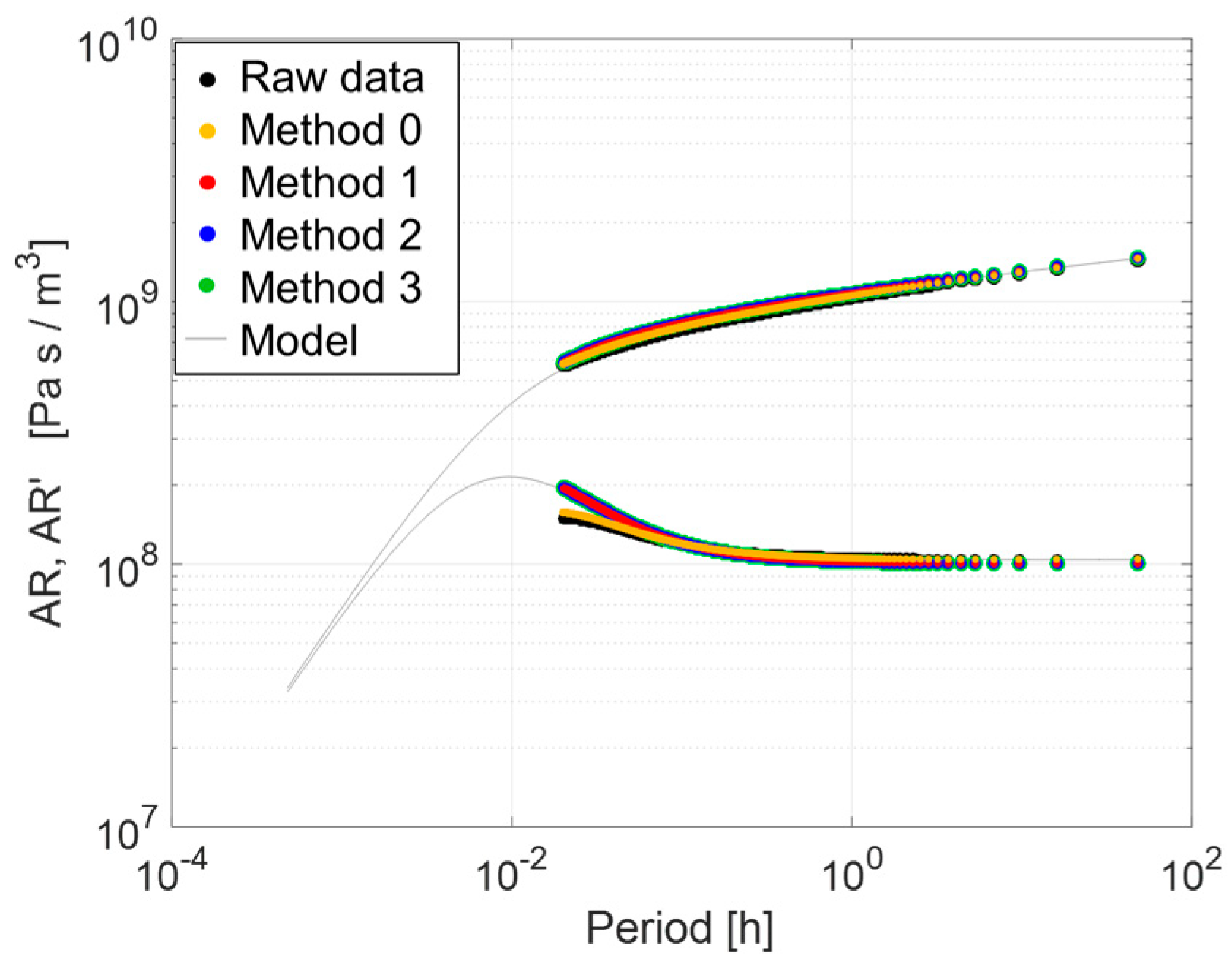
In this case, pressure data periodicity is well preserved; the slight distortion of periodicity induced by initial transient affects the high frequency harmonics only (T < 0.1 h) (Figure 4). Therefore, the derivative of raw data is interpretable.

Linear detrending is not well suited to remove the initial transient effect (Figure 3b). On the contrary, the adoption of any of the heuristic detrending strategies presented in Section 2 improves the pressure data (Figure 3b) and, in turn, the derivative for high frequency components (Figure 4). It is worth mentioning that, in this case, derivatives obtained from detrended data with methods 1, 2 and 3 perfectly overlap.

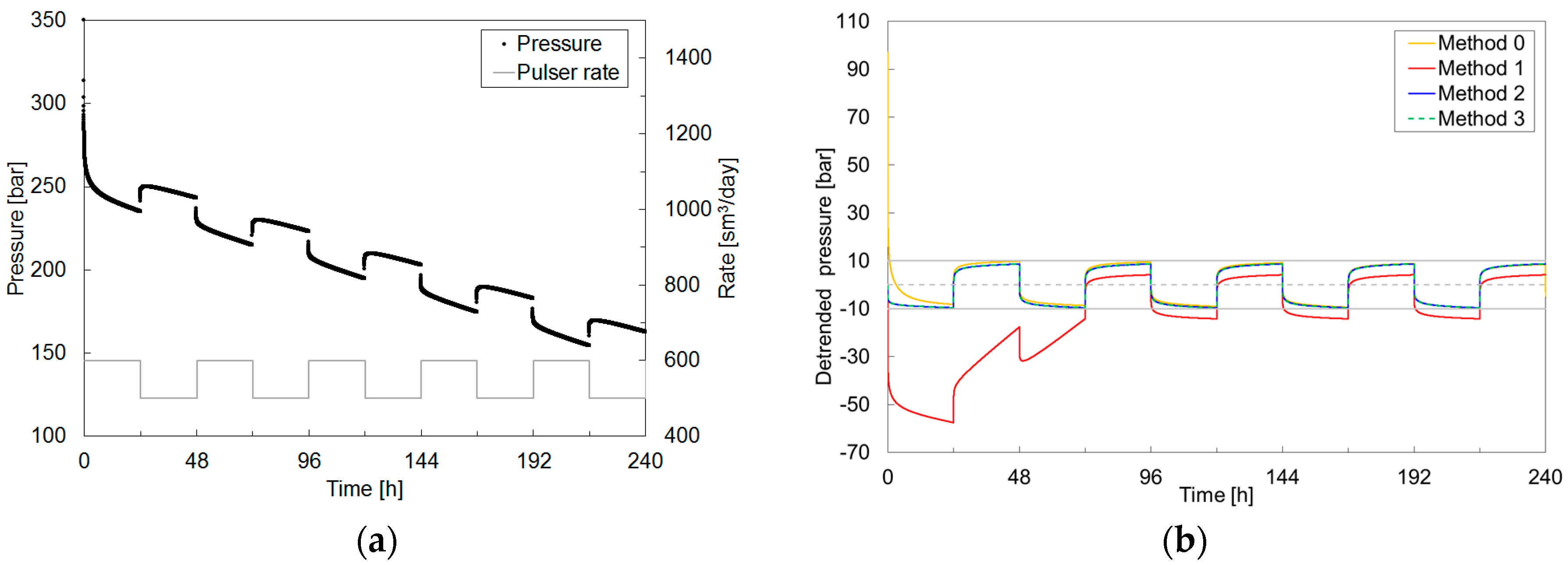
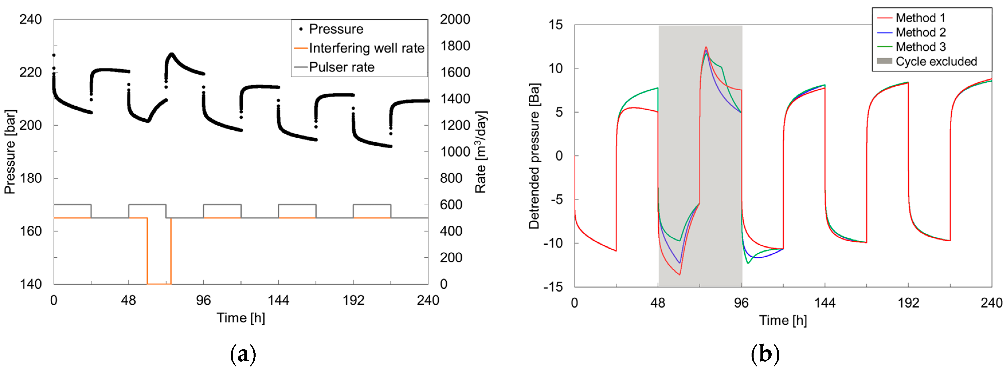
3.2. Synthetic Case 2: Depletion

In the second case, strong reservoir depletion is simulated by considering a closed reservoir of 1000 m × 1000 m with the pulser at the center and introducing a second well (well 1) at a distance of 150 m from the pulser. The additional well is produced with a constant rate of 2000 m³/day. The production from the pulser and from well 1 starts simultaneously and from the initial static conditions. The test is made up of five oscillating cycles in which rates are alternated every 24 h between q₁ = 600 m³/day and q₂ = 500 m³/day (Figure 5a). Two effects mask the periodic trend under the described pressure profile: the depletion trend and a pronounced initial transient. In fact, given that q₀ ≠ q₂, the magnitude of the first pressure transient, corresponding to the first hemicycle (from 0 to $\frac{T}{2})$, is significantly higher than the following pressure oscillations; the more q₀ differs from q₂, the more the initial transient masks the periodic trend in pressure data.

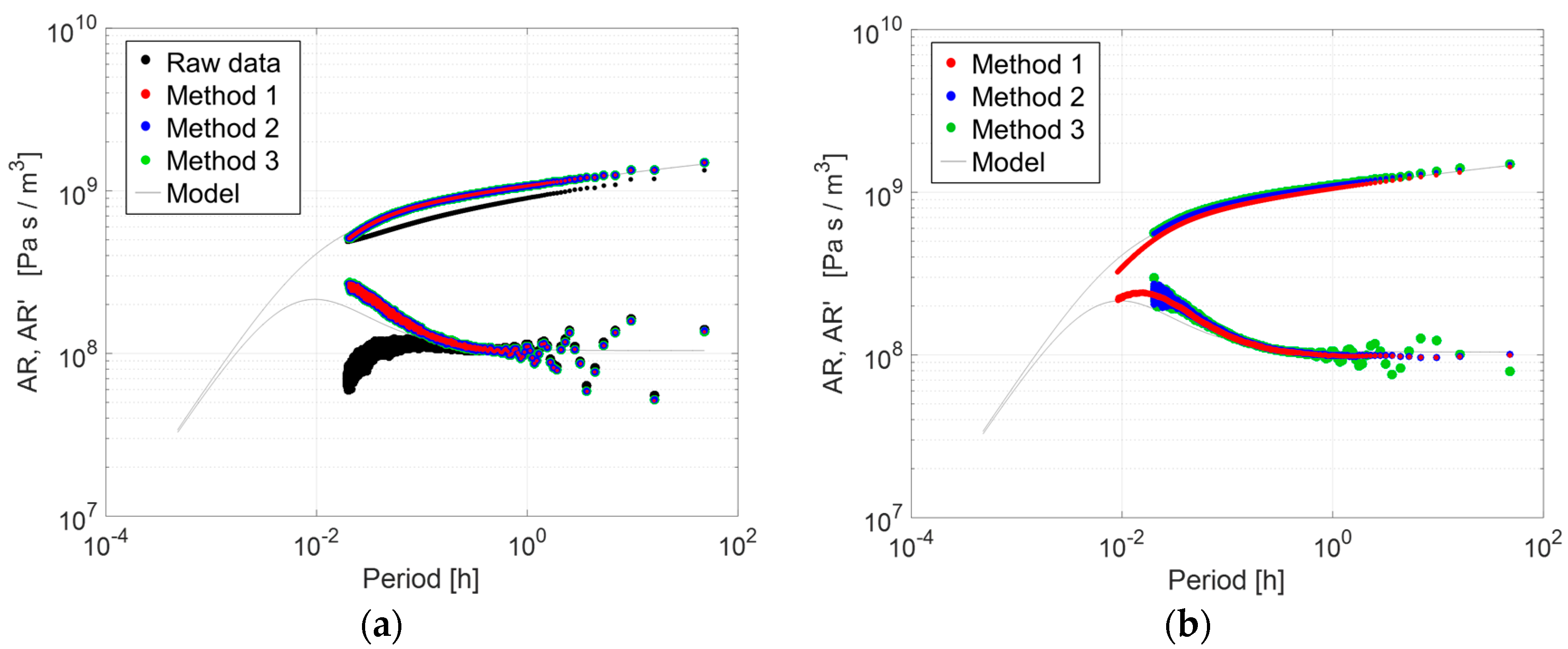
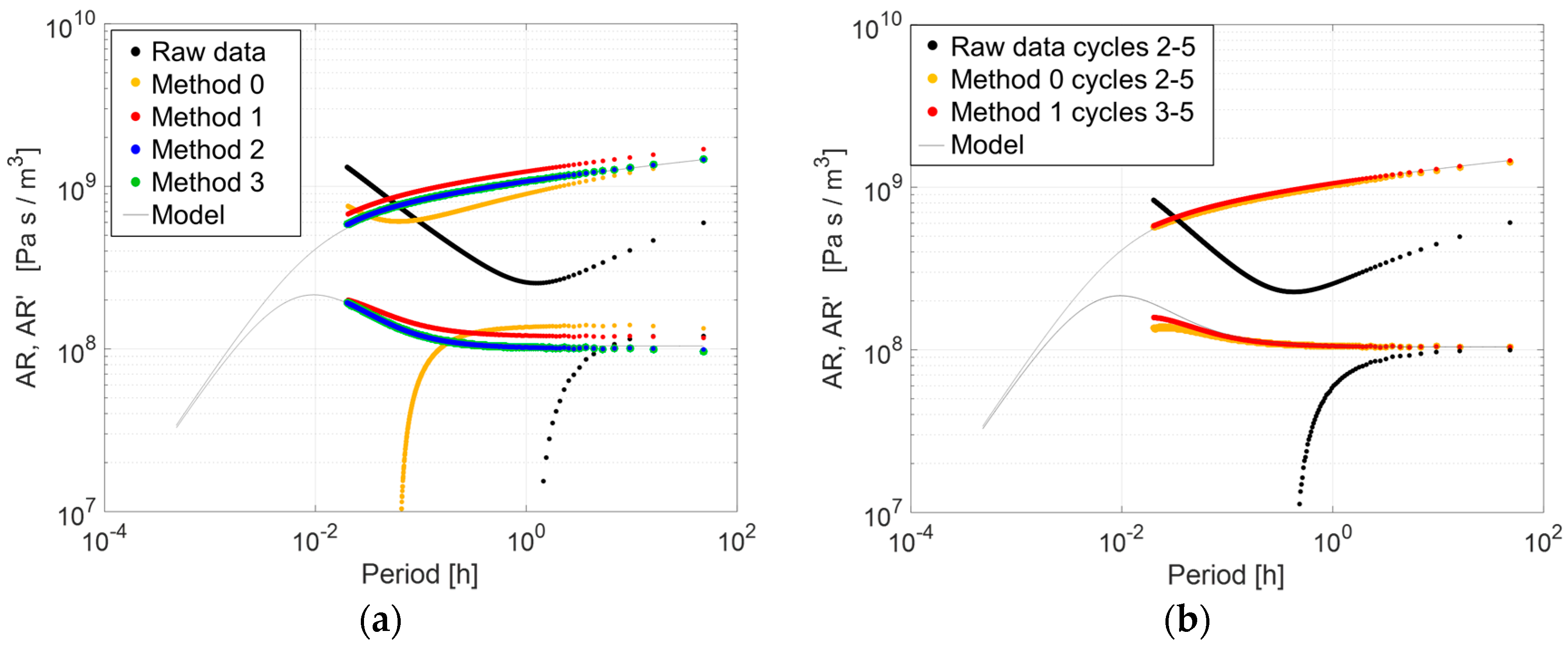
All the detrending strategies presented in Section 2 were applied; the obtained detrended pressures are compared in Figure 5b. Moreover, results are compared on log-log plots in which the amplitude ratio of harmonic components of the pressure and rate spectrums and their derivative (referred to as derivative hereinafter) with respect to the oscillation period are represented. The results obtained for raw data and for the pressure data processed with methods 0, 1, 2 and 3 are represented in Figure 6a. The analysis of the log-log plot (Figure 6a) shows that the derivative of the raw data and of method 0 detrended pressure do not provide reliable interpretation for both high frequencies (low T values) and low frequencies (high T values). Significant errors in the estimation of the kh (underestimation of 25%) and of the skin (S = −2.5 instead of 0) are observed. The derivative of method 1 detrended pressure is affected, as expected, by the first transient and would induce an underestimation of kh of 10% and a slightly incorrect evaluation of mechanical skin (S = 0.5 instead of 0). However, both approaches are still applicable if the number of oscillating cycles is high enough (which is rarely the case in real applications) to allow removing the first cycle, which is strongly influenced by initial transient due to q₀ ≠ q₂ (Figure 6b). However, the removal of initial transient is not sufficient to analyze raw data because the linear trend still masks periodicity. Method 2 and method 3 give very similar results (derivatives overlap), and provide an excellent match with the theoretical model.

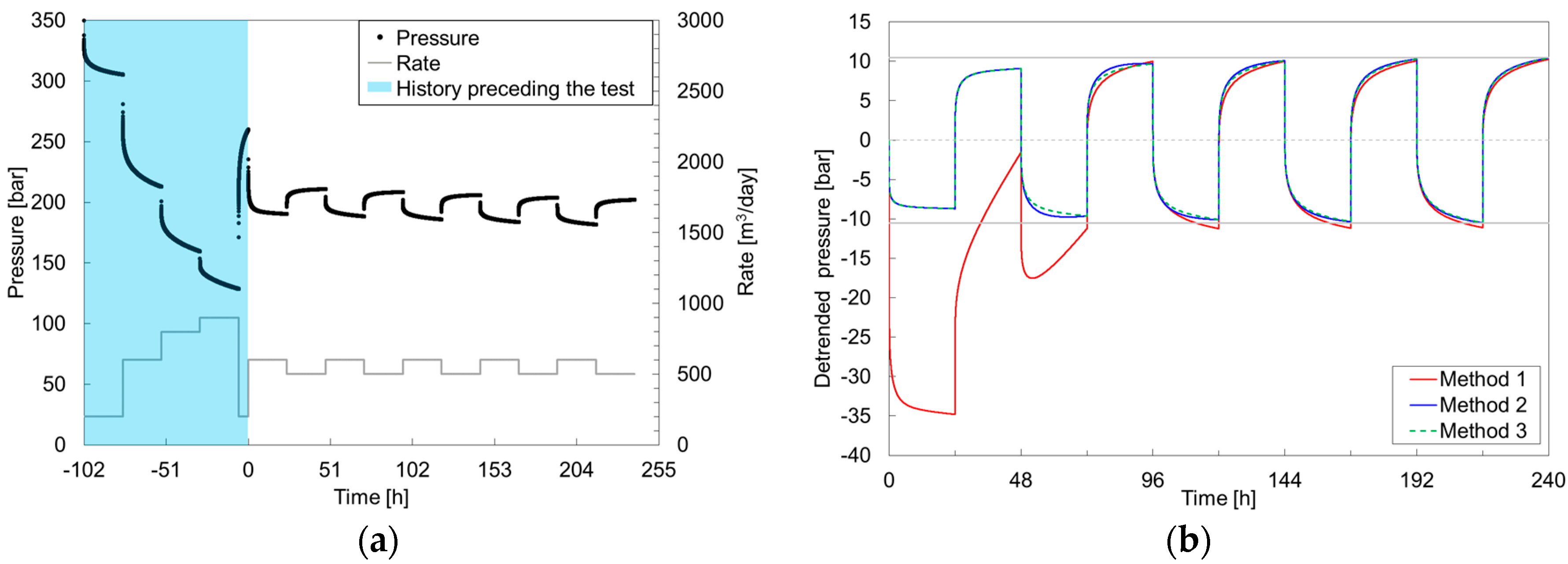
3.3. Synthetic Case 3: Partially Unknown Pre-Existing History

In the third selected case, a single no-flow boundary was defined at a distance of 30 m from the pulser. The well is produced with a changing rate before the test (see Figure 7a); only the very last production rate (q₀ = 200 m³/day) preceding the test is needed for interpretation purposes. The test is made up of seven oscillating cycles in which rates are alternated every 24 h between q₁ = 600 m³/day and q₂ = 500 m³/day (see Figure 7a). The periodic trend is masked by the initial transient under this pressure profile.

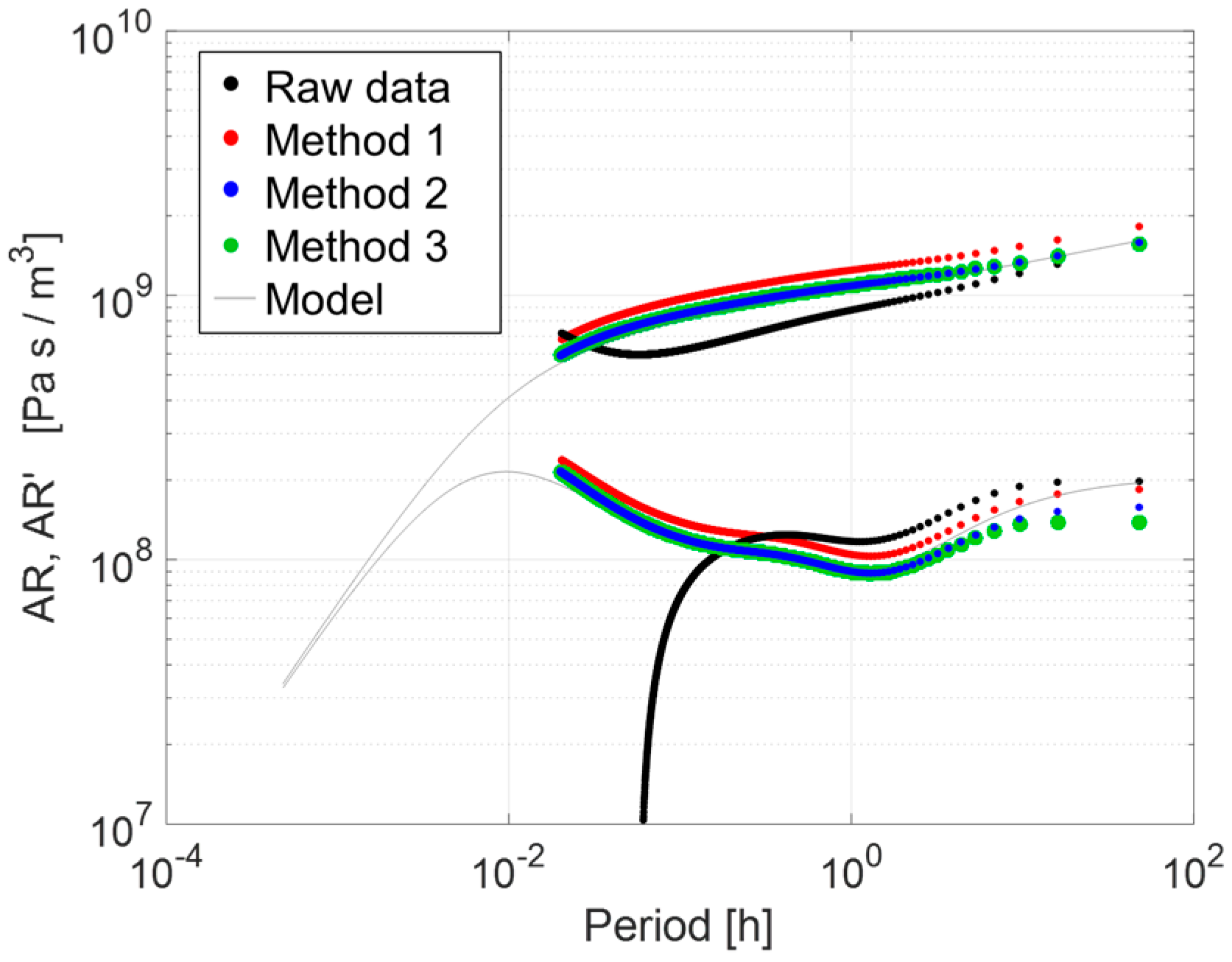
The heuristic detrending strategies presented in Section 2 (method 1, method 2 and method 3) were applied and the obtained detrended pressures are compared in Figure 7b. Moreover, results were compared against raw data in terms of derivative (Figure 8). The derivative of raw data induces an underestimation of the kh value of 20% and an incorrect evaluation of the mechanical skin (S = −1.5 instead of 0). The derivative of method 1 processed data induces an underestimation of kh of 8% and a slightly incorrect evaluation of mechanical skin (S = −0.4 instead of 0). These errors are due to the incorrect detrending of the first cycle, which is strongly influenced by the initial transient due to q₀ ≠ q₂. Methods 2 and 3 provide a reliable derivative (derivatives almost overlap), with a correct identification of the single boundary position. As a result, only the very last production rate preceding the test (q₀) has an impact. Consequently, detrending can be effective if the value of the last production rate prior to the test is known, even when pre-existing production is complicated.

3.4. Synthetic Case 4: Sudden Interference

In this case, an interfering well placed at 80 m from the pulser is introduced. The interfering well produces 500 m³/day, but a sudden well shut in of 15 h occurs during the test. The test is made up of five oscillating cycles in which rates are alternated every 24 h between q₁ = 600 m³/day and q₂ = 500 m³/day (Figure 9a). Furthermore, before the beginning of the test, both the pulser and the interfering wells were producing at a constant rate of 500 m³/day (q₀ = 500 m³/day). Thus, the pre-existing rate (q₀) is equal to the rate of the second oscillation hemicycle (q₂); therefore, no initial transient is observed and the first oscillation cycle is in line with the last two cycles. Conversely, the second cycle is highly affected by the rate change in the interfering well.

The heuristic detrending strategies presented in Section 2 (method 1, method 2 and method 3) were applied; the obtained detrended pressures are compared in Figure 9b. In this case, the detrended pressure of method 1 and method 2 are similar, whereas they differ significantly from the detrended pressure of method 3. In fact, with method 2 (similarly to method 1), the irregularity due to the interfering well is marked and mainly affects the second cycle, while, with method 3, the irregularity due to the interfering well is less marked because it is spread over two cycles. Results were compared against raw data in terms of derivatives (Figure 10a). A rate change in an interfering well lasting less than the oscillation period (or hemicycle) has a strong impact on the derivative, which is highly noisy even at low frequency components; as a consequence, the horizontal stabilization representing radial flow geometry in a transient regime (Infinite Acting Radial Flow–IARF) is hardly detectable.

Successively, the most irregular oscillation period (cycle 2) was excluded from the analysis (Figure 9b) and the improvement in derivative interpretability is shown in Figure 10b. Method 3 is not well suited for detrending such scenario because it spreads the irregularity over more oscillating cycles, thus making the exclusion of the more affected cycle less effective.

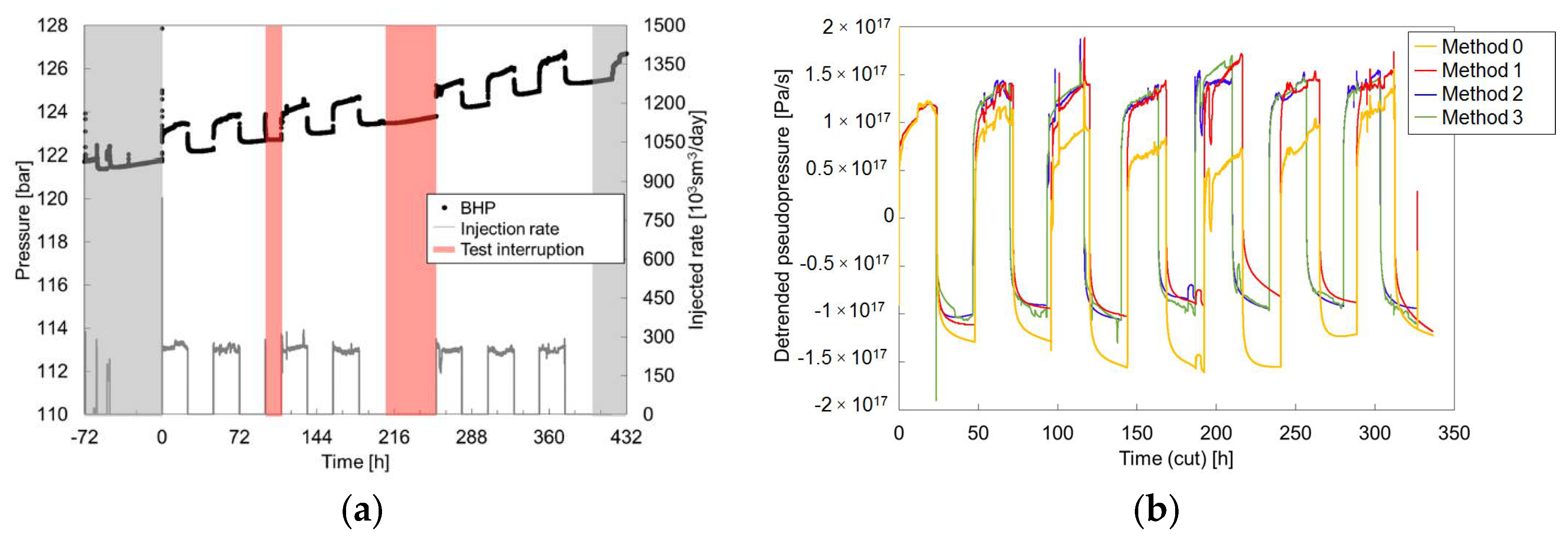
3.5. Real Case: Temporary Interruption of the Test

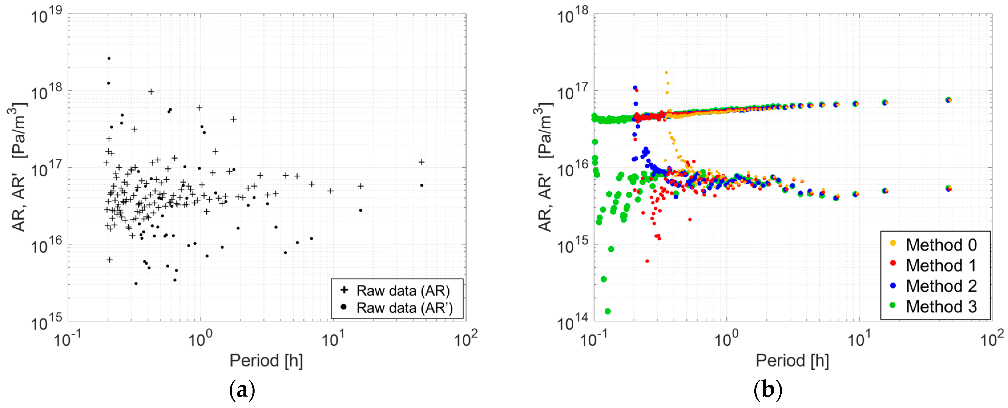
A gas storage well was tested during the injection campaign without interruption of the activities from the other wells of a field in Italy. The test design was a rate of 250,000 m³/day for 24 h alternated with wells shut in of the same duration (Figure 11a). Significant rate instability/fluctuations during the injection periods were due to operational and technical reasons. Downhole pressure data was recorded every 10 s while rate data was recorded every 30 s; rate data was resampled according to pressure data. Due to operational issues, after the first two cycles, the test was temporarily interrupted (the well was shut after 1.5 h of injection and remained shut for 13.5 h) and was interrupted again for 47.5 h (extended well shut in) after the following 1.5 cycles. Consequently, the overall test periodicity was seriously compromised and only few consecutive cycles were available. Except for the two test interruptions aforementioned, in most hemicycles, rate changes were anticipated/postponed with respect to the design by a few to a maximum of 40 min. As a consequence, the raw test data does not meet the HPT interpretation methodology requirements of regular periodicity. In fact, when applying the Fourier analysis to the original data, a scattered derivative is obtained (Figure 12a), which is clearly not interpretable.

All of the four detrending techniques described in Section 2 were applied to pseudopressure data. Method 0 and method 1 were suitable in this context because q₂ = q₀ = 0, thus no initial transient was observed. However, detrending with method 0 was not completely successful because the slope of the linear trend changed after the second test interruption.

After detrending, the data portion related to the two test interruptions were removed; for method 2 and method 3, which gave more regular oscillations, a further regularization was applied by removing all the data portion related to hemicycle duration greater than the minimum one (23.34 h). The detrended pseudopressure data obtained from each methodology are compared in Figure 11b. Derivatives of detrended data are shown in Figure 12b. Comparison between Figure 12a,b shows that the application of the detrending methodologies improves the derivative quality, making the horizontal stabilization clearly detectable and therefore allowing kh estimation. Furthermore, among the detrending strategies, method 3 allowed better extraction of early time information. The residual scattering observable on the derivatives for methods 2 and 3 is due to rate instabilities and for methods 0 and 1 to the residual flow period duration irregularity as well.

4. Discussion

The cases analyzed in Section 3 show that, only in case 1, characterized by negligible well interference, small overall pressure decline and negligible initial transient (q₀ = q₂), the Fourier analysis of HPT raw pressure data is feasible. In fact, in the other cases (well interference, significant overall pressure decline, initial transient due to previous history), the derivative obtained from raw data analysis in the frequency domain was either not interpretable or provided interpretation results affected by errors on kh and/or skin estimate. In such scenarios, the use of a detrending algorithm as a data preprocessing is compulsory.

The detrending strategies allowed for extracting from pressure raw data the periodic component that was masked by non-periodic effects, and thus enhanced the quality of the derivative. Based on the results, the adequate detrending strategies for each scenario are listed below:

• in the presence of a significant pressure decline, either due to reservoir depletion or constant well interference, all the considered strategies are effective.
• if a significant initial transient is observed, because of rate history prior to the test (es. q₀ << q₂), method 2 or method 3 can be successfully adopted.
• if any oscillation cycle (or hemicycle) is significantly altered by an interfering well, method 1 or method 2 can be adopted to allow the exclusion of anomalous cycle(s) from the Fourier analysis.
• if any hemicycle is significantly longer/shorter than the design, as in the case of a temporary suspension of the test, detrending with method 1, method 2 or method 3 allows the exclusion of the redundant parts of the hemicycle(s)/the exclusion of the short cycle(s) from the Fourier analysis.

5. Conclusions

For cases in which conventional well tests are not doable, be it that interruption of reservoir production or production from the tested well is out of the question, the complementary well test methodology Harmonic Pulse Test has been designed. Nonetheless, HPT should not be seen as a replacement for standard or conventional well testing, but rather as a valid option for cases like the aforementioned. To make the best of the information given by the interpretation of an HPT in the frequency domain, the aperiodic pressure decline trend due to initial transient, well interference, reservoir production, boundaries, should be recognized/reconstructed and removed from the pressure signal to identify, in theory, the pure periodic component. The application of detrending methodologies can offer an approximation of the periodic component of a pressure signal. Authors presented four detrending methodologies. Two of them, named method 2 and method 3, were developed by the authors and are based on the application of superposition principle adopted to recognize and separate the periodic component form the aperiodic one. The four detrending methodologies were discussed, compared and validated by their application to several synthetic cases as well as a real case, each representing a possible scenario featuring criticalities that could affect and reduce the reliability of the interpretation process of an HPT. The different methodologies were compared in terms of derivative of the amplitude ratio on the log-log plot.

Results showed that, for certain critical scenarios (i.e., when the periodicity is affected by significant pressure decline, initial transient, well interference, errors in timing of rate changes), the application of detrending methodologies is necessary to avoid misleading results from the interpretation of test raw data. In particular, linear detrending (method 0) is effective in removing the pressure trend induced by field depletion and constant well interference but cannot tackle transient effect related to preexisting rate history or ongoing production changes. Conversely, the detrending algorithms based on a heuristic approach, i.e., method 2 and method 3, are very effective to remove both. Finally, the analysis of detrended data can be further improved by excluding anomalous cycles, i.e., cycles that do not respect the designed test periodicity, such as in the case of well interference and/or temporary interruption of the pressure pulses during the execution of the test. This result was confirmed by application of the detrending algorithm to a real HPT on a gas storage well, during which the data periodicity was compromised by temporary interruptions due to operational constraints; data pre-processing ensured preservation of pressure periodicity, thus enhancing the quality of the derivative of low frequency harmonic components (corresponding to middle time in the conventional derivative).

The quality of the results from HPT interpretation can be considerably improved by adopting an effective detrending strategy and by doing so there is the real possibility of overcoming the limitation in applicability of HPT due to the difficulty of imposing a regularly pulsing rate for the whole test duration (typically lasting several days). In other words, detrending offers the opportunity of making HPT appealing for well performance monitoring, which is particularly important for gas storage field management.