The Value of Day-Ahead Coordination of Power and Natural Gas Network Operations

Abstract

The operations of electricity and natural gas transmission networks in the U.S. are increasingly interdependent, due to the growing number of installations of gas fired generators and the penetration of renewable energy sources. This development suggests the need for closer communication and coordination between gas and power transmission system operators in order to improve the efficiency and reliability of the combined energy system. In this paper, we present a co-simulation platform for examining the interdependence between natural gas and electricity transmission networks based on a direct current unit-commitment and economic dispatch model for the power system and a transient hydraulic gas model for the gas system. We analyze the value of day-ahead coordination of power and natural gas network operations and show the importance of considering gas system constraints when analyzing power systems operation with high penetration of gas generators and renewable energy sources. Results show that day-ahead coordination contributes to a reduction in curtailed gas during high stress periods (e.g., large gas offtake ramps) and a reduction in energy consumption of gas compressor stations.

1. Introduction

Electricity and natural gas transmission networks in the United States (U.S.) are interconnected energy infrastructures whose operation and reliability depend on one another to a large extent. The most significant interconnections between both energy systems exists at natural gas fired power plants (GFPPs) and electric driven compressors (EDCs) in gas compressor stations. GFPPs represent generation entities in the power system, while at the same time they represent large consumers in the natural gas network. Gas generators require a minimum delivery pressure for operation, which, if violated, can lead to curtailment of gas offtakes, and in the worse case to a complete shut down of the GFPP [1,2]. EDCs, in contrast, represent electric loads in the power system, which are utilized by electric drivers to propel compressors in gas compressor stations in order to increase the gas pressure for pipeline transportation. In this paper, we focus mainly on the impact of GFPPs on the operation of the combined energy system.

The interconnection and interdependency between power and natural gas networks has become stronger in the past decades with the increase in the total installed capacity of GFPPs. U.S. natural gas deliveries to electric power consumers has increased by 60% between 2006 and 2016 [3]. This trend is partly due to the increase in electricity consumption, unconventional gas extractions, greenhouse gas (GHG) emission concerns, and, lately, lower natural gas prices. It is expected that this trend will continue along with the future increase of renewable energy sources (RES). The need for flexibility in power systems increases with higher penetrations of variable RES, such as wind and solar power, due to their variable and uncertain nature. This flexibility can be partially mitigated, among other options, by fast-reacting gas-fired power plants. These power plants are operated differently under high RES penetrations by ramping upward and downward more frequently and to a larger extent, and by starting up and shutting down more often.

The times during which, and the extent to which GFPPs extract natural gas from the gas network, and the extent to which they do so, depend strongly on their generation schedule. In other words, higher RES penetrations in the power system will not only impact how GFPPs interact within the power system, but they will also impact how they interact with the natural gas network. For instance, a large wind or solar power forecast error could be the cause of a large change in gas demand to be handled within the natural gas network operational and flexibility boundaries.

Traditionally, gas and power transmission systems have been planned and operated independently, due to the relatively weak coupling between both systems in the past. However, the growing interdependency between the energy vectors suggests the need for models and tools to study how this trend may impact the operation of both systems, and how to improve the coordination between gas and power transmission system operators (TSOs) to increase operational efficiency and system reliability.

The research area of gas and power system interdependency is relatively new. Recently, a number of studies in this area addressing the operational coordination between both energy carriers have been published. In [4], the authors review the research works carried in the optimization of natural gas transportation systems, specifically in the areas of short-term basis storage, pipeline resistance and gas quality satisfaction, as well as the challenges faced considering the steady state and transient models. In [5,6], the authors introduce an optimization model for the combined simulation of gas and electric power systems, where both systems are interconnected through GFPPs. The model consists of a DC-OPF model for the power system and a transient hydraulic optimization model for the gas system. However, the authors do not consider important generator constraints such as the ramp rate and start-up and shut-down times and costs that are essential for making day-ahead and real-time unit commitment decisions. Nevertheless, the results presented by the authors indicate that increased coordination between gas and power system networks is required to ensure security of supply and economic efficiency, particularly, under highly stressed conditions.

In [7], a security constrained economic dispatch model for integrated natural gas and electricity systems was presented considering both wind power and power-to-gas processes. The authors use a transport model to represent gas flow in pipelines, which does not properly account for changes in linepack and pressure. In [8], a bi-level optimization model for day-ahead coordinated operation of an electricity network and a natural gas system is developed. The coordination of both systems is carried out under steady state conditions, and, as such, cannot resolve the gas system impacts from dynamic behavior such as wind ramping. In [9], the authors developed a framework for modeling and evaluating integrated gas and electric network flexibility, taking into consideration changes in the heating sector. The constraints imposed by the gas network’s local flexibility limits are particularly considered. The authors use a DC-OPF approach to model the electric power system and both steady-state and transient models for the gas system. Chaudry et al. [10] present a multi-time period combined gas and electricity optimization model that highlights the consequences of failure of important facilities in a combined network. Whilst a transient approach was used for the gas network, a direct current power flow (DC-PF) approach was used for the electric network. In [11], the authors proposed a bi-level mathematical model for the security-constrained unit commitment problem using fuzzy logic to model the uncertainty of the gas system. A steady-state approach was used for the gas network and a DC-PF was used for the electric network. Bai et al. [12] present an interval optimization model based on an operating strategy, which considers demand response and wind power uncertainty. A steady-state mathematical model was applied for the gas system, while a DC-PF model was used for the power system. In [13], a short-term stochastic model was developed to coordinate natural gas and wind energy units in power systems considering the constraints of the natural gas networks, such as emission limits and wind energy variability. The authors use a DC-PF approach to model the electric power system, while a steady state model was used to describe the operation of the natural gas system.

The majority of the models addressing the coordination between gas and power systems in the literature use steady state models to describe the operation of the gas system, which is inadequate for operational analysis since the changes in linepack and the time evolution of pressures are not captured appropriately in steady state models. These phenomena are important considerations to account for in order to account for the pressure limits in the gas system when operating a large number of gas fired generators. Moreover, most studies do not distinguish between the day-ahead scheduling and real-time operation in the gas and power systems, which can lead to an underestimation of the flexibility needed in the operation of both systems. In addition, most studies do not use a complete model for the gas system. For instance, the inertia and gravitational term in the pipe flow equation (momentum equation), as well as key gas system facilities such as underground gas storage and liquefied natural gas (LNG) regasification terminals are usually neglected. The latter are particularly important when studying the operation of gas generators, since they provide additional flexibility to react to fluctuations in supply and demand.

In this paper, we close some of the gaps identified in the literature by developing a co-simulation platform to study how the coordination between gas and power system TSOs may improve the operational efficiency and reliability of interconnected gas and electric power transmission networks. The co-simulation platform consists of a steady-state direct current (DC) unit commitment and economic dispatch model to simulate bulk power system operations and a transient hydraulic model to simulate the operation of bulk natural gas pipeline networks. Here, a steady-state electricity model combined with a transient natural gas model is appropriate because the dynamics of the electricity system are orders of magnitude faster than the dynamics of natural gas system, and our focus is on natural gas system dynamics. The system models are implemented in two separate simulation environments, namely, PLEXOS [14], a production cost modeling tool for electric power systems and SAInt-Scenario Analysis Interface for Energy Systems [15,16,17,18,19,20]—an energy systems integration tool that includes a standalone steady-state and transient hydraulic gas simulator. The data exchange between the simulations is conducted by an interface that maps the power generation of gas generators in the power system with the corresponding fuel offtake points in the gas system. The information exchanged between both simulation environments is:

• the day-ahead (DA) and real-time (RT) fuel offtakes of gas fired generators in the electric power system and
• the fuel offtake constraints imposed by the gas network system on the power system, due to pressure restrictions in the gas system.

The goals of this paper are:

• to develop a combined power–gas test system that can be used to test and benchmark different methods for addressing the simulation of interdependent gas and electricity systems,
• to show the importance of considering the restrictions imposed by gas transmission networks when operating a large number of gas fired generators in the electric power system, and
• to demonstrate the importance of coordination between gas and power TSOs to improve the efficiency and reliability of the combined energy system.

To achieve these goals, the paper is structured as follows. In Section 2, we give a brief introduction to the gas and power system models used in this study and present the structure of the co-simulation platform that coordinates between the two simulation environments. In Section 3, we apply the co-simulation platform to study three scenarios with different wind and solar penetration levels and compare how the day-ahead coordination between the gas and power systems may impact the operation of both energy systems. Finally, in Section 4, we discuss the results and give and provide a look at future studies that can be developed from the models and results presented in this paper.

2. Methodology

Electric transmission networks in the U.S. are managed by vertically integrated utilities and Independent System Operators/Regional Transmission Organizations (RTOs) depending on the region. These entities are responsible for clearing the regional electricity market and for scheduling the operation of power system generators to balance power system loads. In most U.S. electricity markets, the commitment and dispatch of generators are scheduled in two steps, namely, the day-ahead scheduling (DA) and the real-time balancing (RT). The first step involves clearing the day-ahead market 24 h prior to the operating day, using a unit commitment (UC) model to determine when and which generation units will be operated during the operating day and the scheduled generation of these committed units. This is done considering their operational costs and constraints, the projected power system loads and reserve requirements. The RT, on the other hand, involves clearing the real-time intra-day market by solving a real-time UC and ED model typically every 5–15 min.

Gas transport systems, in contrast, are managed by gas transmission companies, which are responsible for ensuring reliable and economic operation of the gas transmission system. In a gas market, day-ahead and intra-day bi-lateral agreements based on steady rated nominations exist between gas traders (shippers) and transmission system operators. The day-ahead nominations are used by gas transmission companies to develop a day-ahead operational schedule before the actual operating day, which involves determining the cost-optimal settings of controlled facilities, such as compressor stations, regulator stations, valves and gas storage facilities and at the same time ensuring that pressure limits and linepack requirements are fulfilled during the operating day. In real-time operation, the control of the gas system is adjusted in response to changes in demand and supply based on practical experience and the evaluation of a large set of look-ahead-scenarios using transient hydraulic simulation models. In the past, these changes were relatively small and could be managed quite well, since the majority of gas customers were local distribution companies (LDC) with firm contracts and nearly constant hourly gas offtakes throughout the operating day. Presently, power generation companies account for more than half of total gas offtakes in some market regions in the U.S. These customers usually purchase interruptible contracts and may ramp-up and ramp-down more frequently and unexpectedly during the operations. This operating mode creates challenges for gas TSOs since gas generators may start-up and withdraw gas with short notice, leaving the gas TSO a limited amount of time to react to these changes. If this situation occurs in a moment where the gas system is in a stressed state, the gas TSO will typically curtail the gas offtakes of customers with non-firm contracts (e.g., GFPPs) to maintain reliable system operations and to ensure the delivery of gas to customers with firm contracts (e.g., LDC). Such undesired situations could be reduced and/or avoided if changes in power and natural gas systems are communicated and coordinated well in advance.

In this section, we present a co-simulation platform to examine how the coordination between gas and power TSOs may improve the reliability and efficiency of interdependent gas and electric power system operation. In Section 2.1, we provide an overview of the power system simulation model and the power system network used for the case studies. Section 2.2 explains the model used for simulating the gas system and the properties of the gas network model developed for the case study. Finally, Section 2.3 is dedicated to detailing the co-simulation platform and the different simulation runs conducted for the case studies.

2.1. Power System Model

Bulk power system operations are simulated by running a production cost model in PLEXOS (6.4, Energy Exemplar, North Adelaide, Australia), a commercial power system modelling tool. The model solves a mixed integer linear optimization problem to optimize unit commitment and economic dispatch decisions subject to energy balance, reserve requirements, generation, transmission, and demand constraints. The model simulates bulk power system operations by modelling DA commitment decisions and the resulting RT generation re-commitment and dispatch decisions. This is done by performing two simulations, one for day-ahead and one for real-time. Day-ahead commitment decisions of electricity generators that cannot be recommitted in real time are passed and enforced from the day-ahead simulation to the real-time simulation. Day-ahead commitments are simulated considering day-ahead load, wind power, and solar power forecasts. These can lead to sub-optimal commitment decisions, especially in situations when net load (load minus wind and solar power) forecast errors are large. When net load is under forecasted, generators that were not committed in the day-ahead stage, and that have fast startup times (e.g., natural gas combustion turbines), will be recommitted and started in real-time to meet the electricity load not accounted for.

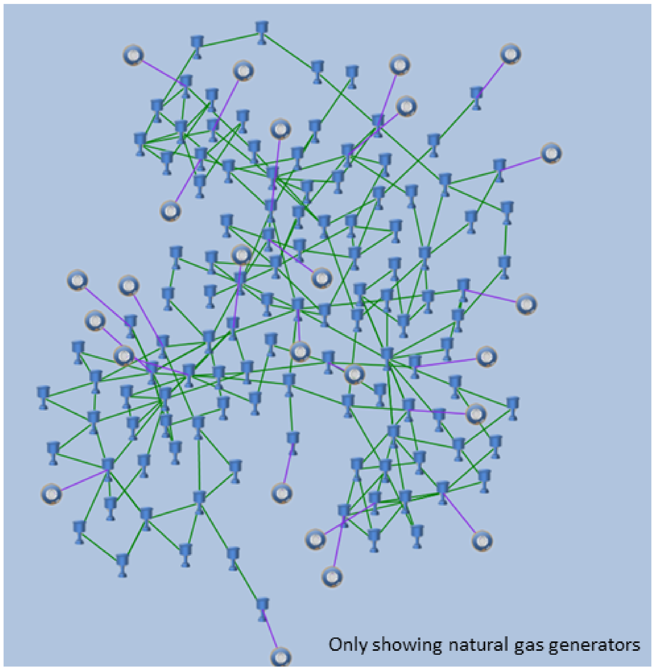
In this paper, we model a test power system defined in Figure 1.

The test system is based on the IEEE 118-bus test system. The hourly load profile utilized is the historical load from the San Diego Gas and Electric balancing authority area for the year 2002 [21]. Time-synchronous wind data and forecasts were utilized from areas near San Diego from the Wind Integration National Dataset Toolkit [22]. 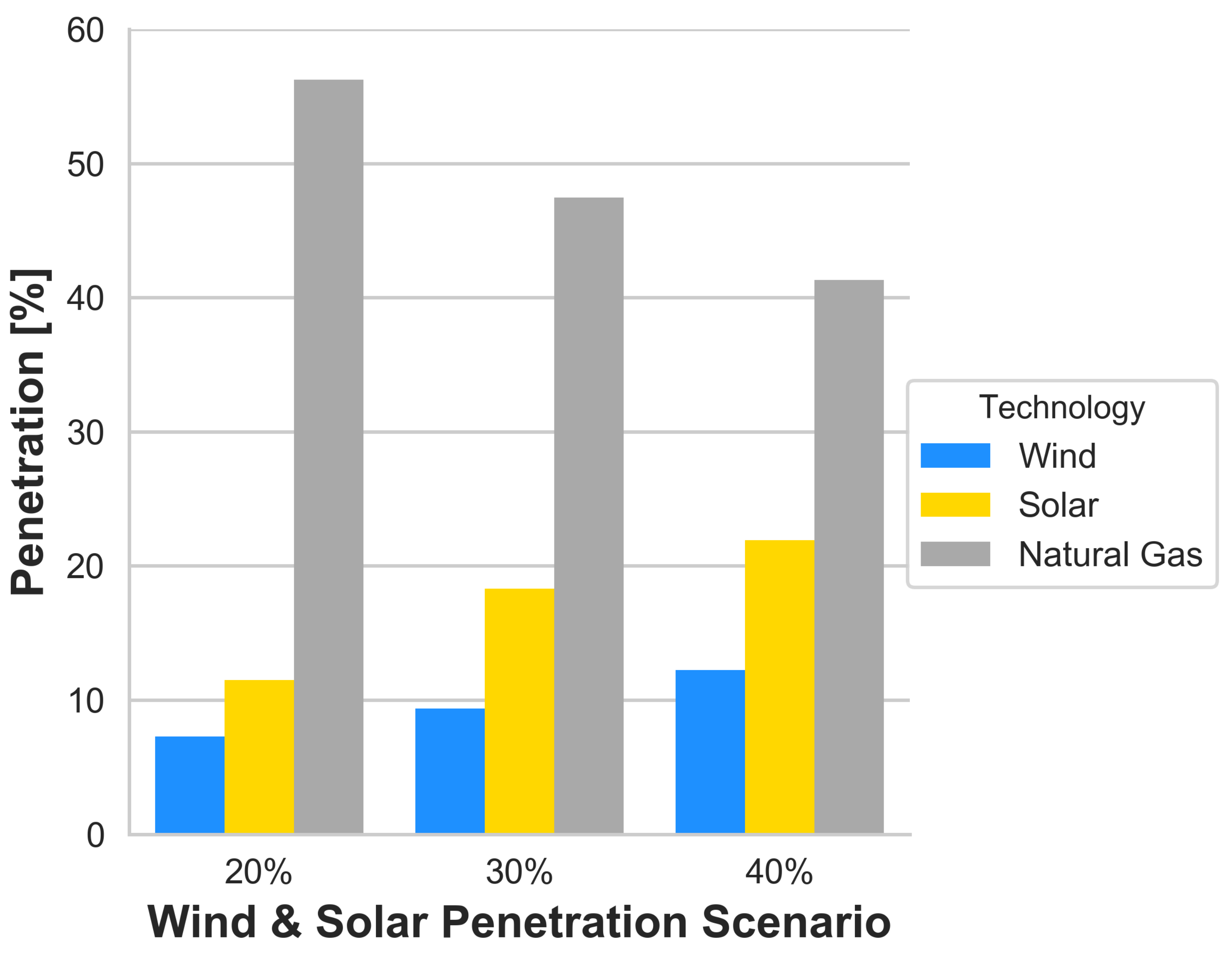Time-synchronous solar power data and forecasts were based on data available from the National Solar Radiation Data Base [23] and created in [24]. The test system is designed with an electricity generation mix that resembles the current California generation mixture with high shares of gas-driven electricity generation capacity. Moreover, the test system can be modeled under three different scenarios in terms of wind and solar power penetration: 20%, 30%, and 40% in annual energy terms.

Table 1. Power test system generation mix.

Generation Type	Number of Generators	Installed Capacity (MW)
Hydro	4	1035
Nuclear	1	238
Coal	2	52
Geothermal	2	176
Biomass	5	76
Biogas	2	45
Natural Gas	25	4395
Oil	2	43

shows the number of conventional generators included in the modeled test power system, as well as their combined installed generation capacity. The model also includes 10 wind power plants and 10 solar photovoltaic power plants that have different installed generation capacity depending on the penetration scenario.

The 25 gas power plants included in the model are of four types: steam turbine, combined cycle, combustion turbine, and internal combustion engine. The first two types are committed in the day-ahead simulation due to their longer startup times, while the two latter types can be recommitted in the real-time simulation. They can all be redispatched in RT, as long as ramping, minimum and maximum generation constraints are respected. In this paper, we examine the value of considering natural gas network constraints on the day-ahead power plants commitment decisions.

2.2. Gas System Model

The operation of gas networks is inherently dynamic. Demand and supply are constantly changing and the imbalance between these two quantities is buffered by the quantity of gas stored in pipelines, also referred to as linepack. The linepack is proportional to the average gas pressure and gives the gas system additional flexibility to react to short-term fluctuations in supply and demand. Thus, knowing the level of linepack and the pressures in the gas transport system is crucial for managing the operation of gas network. According to the law of mass conservation the linepack in a gas pipeline can only change in time if there is an imbalance between total supply and total demand, also referred to as the flow balance. This, in turn, implies that, in order to reflect the changes in linepack, and thus the changes in pipeline pressure, a steady state model, where the flow balance is always zero (i.e., total supply is equal total demand), is inadequate. Thus, for operational studies, where the time evolution of linepack and pressure are crucial, a dynamic model for the gas system is necessary.

In this paper, we reflect the behavior of the gas system by a transient hydraulic model, which is implemented in the simulation software SAInt (1.2, cleaNRGi^® Solutions GmbH, Essen, Germany). SAInt contains a model for the most important facilities in the gas system, such as pipelines, compressor stations, regulator stations, valve stations, underground gas storage facilities, LNG terminals and other entry and exit stations. The mathematical models implemented in SAInt have been published in [16,17,18,19,20], where a detailed description and application of the simulation tool are given. Furthermore, the accuracy of the transient gas simulation model has been successfully benchmarked against a commercial gas simulation tool and other models in the scientific literature [16,17].

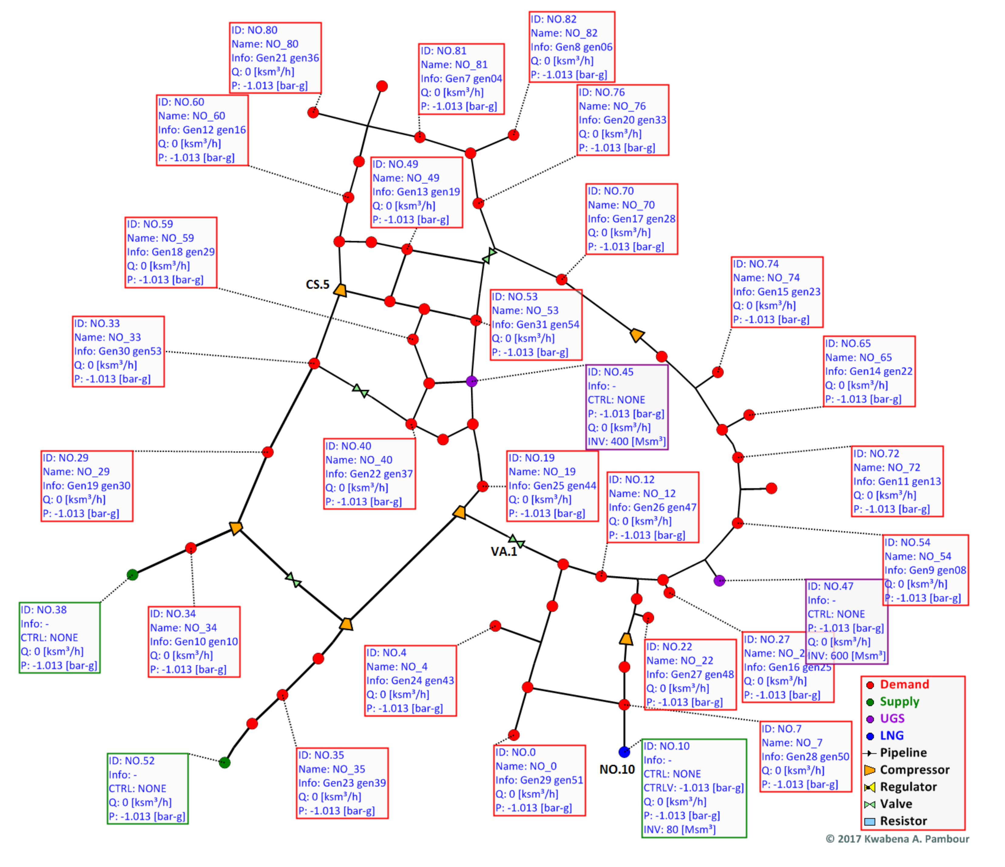
The topology of the gas network model (GNET90) used in this study is depicted in Figure 2 and the basic properties of the network are listed in

Table 2. Properties of the GNET90 gas network.

Property	Value	Unit
Nodes	90	-
Pipelines	90	-
Compressor Stations	6	-
Valve Stations	4	-
Underground Gas Storage Facilities (UGS)	2	-
LNG Regasification Terminals	1	-
Gas Fired Power Plants (GFPP)	25	-
City Gate Stations (CGS)	17	-
Cross Border Import Stations (CBI)	2	-
Total Pipe Length	3734	(km)
Total Geometric Pipe Volume	1,539,221	(m3)
Total Available Compression Power	240	(MW)
Min. Pipe Diameter	600	(mm)
Max. Pipe Diameter	900	(mm)
Min. Elevation	0	(m)
Max. Elevation	1118	(m)

.

The gas model has a total pipe length of 3734 km, which is subdivided into 90 pipe elements. The model includes six compressor stations for increasing the gas pressure for transportation and four valve stations for controlling the gas stream, and islanding sections of the network. The pipe and non-pipe elements are interconnected at 90 nodes, where gas can be injected or extracted from the network. The 90 nodes contain three supply nodes, which include one LNG Terminal with a working gas inventory of 80 Msm³, two underground gas storage facilities with a total working gas inventory of 1000 Msm³, 46 gas offtake stations, which include 25 GFPPs and 17 city gate stations (CGS). The minimum delivery pressure at each GFPP is set to 30 bar-g, while the minimum pressure at each CGS is set to 16 bar-g. Gas offtake stations with minimum delivery pressure limits are subject to gas curtailment if their corresponding nodal pressure cannot be maintained above the pressure limit for a given scheduled offtake. The difference between the scheduled offtake and the actual delivered quantity are integrated over the simulation time window to yield a quantity referred to as gas not supplied (GNS), or energy not supplied if multiplied with the gross calorific value (GCV).

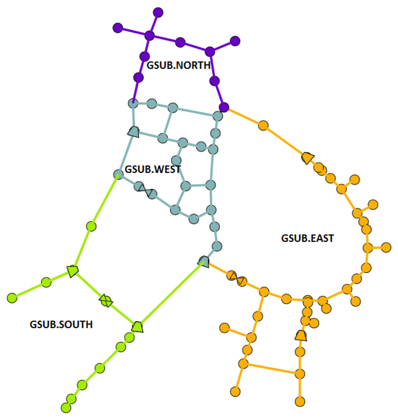
Furthermore, the gas system is divided into four subsystems, as shown in Figure 3.

The parameters of the subsystems (e.g., linepack, minimum pressure, etc.) are used to monitor and control the pressure and linepack of specific regions in the network and to change the control modes and set points of controlled facilities (e.g., compressor stations, valves, etc.) to maintain system operating conditions, similar to actual gas network operations.

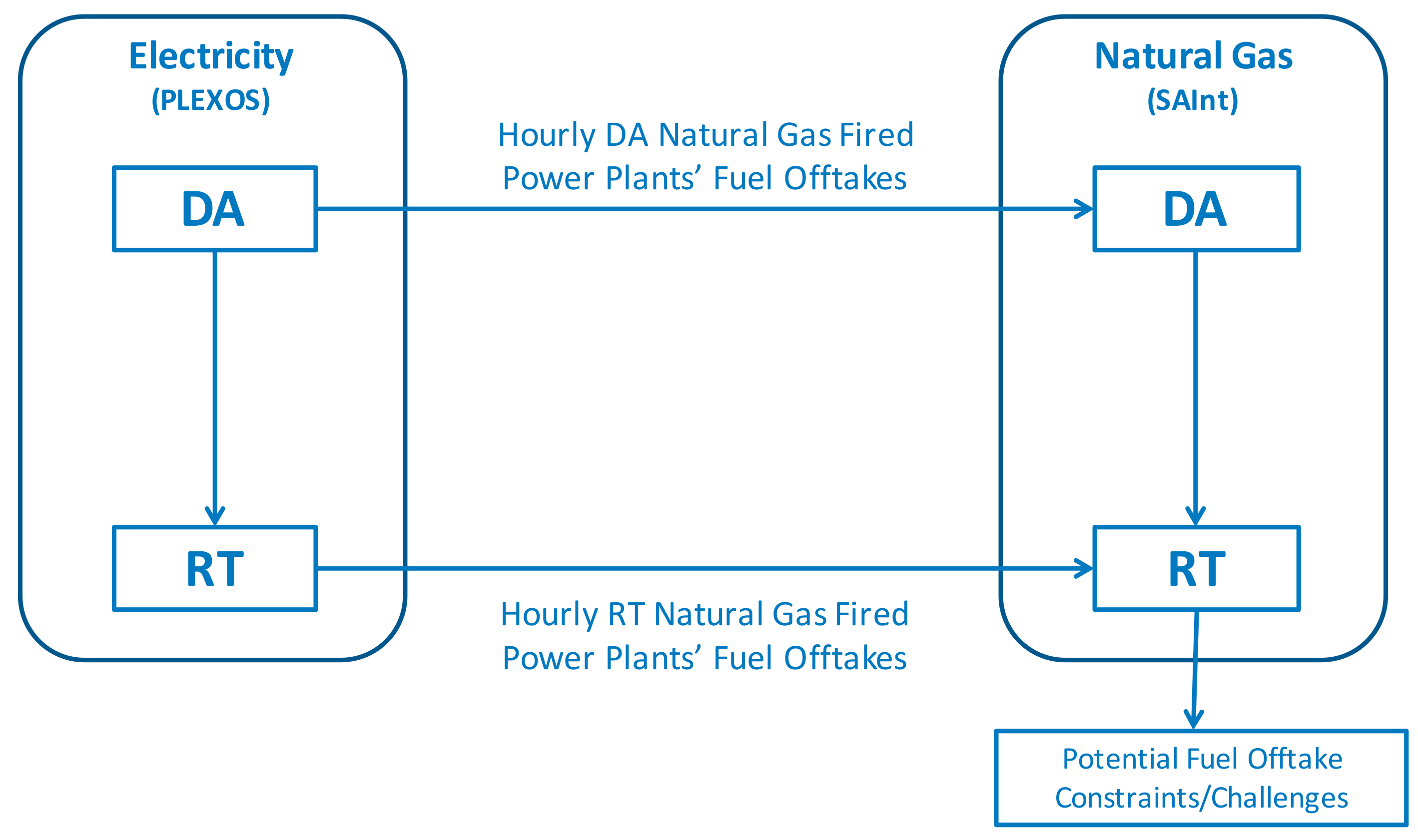
2.3. Co-Simulation Platform

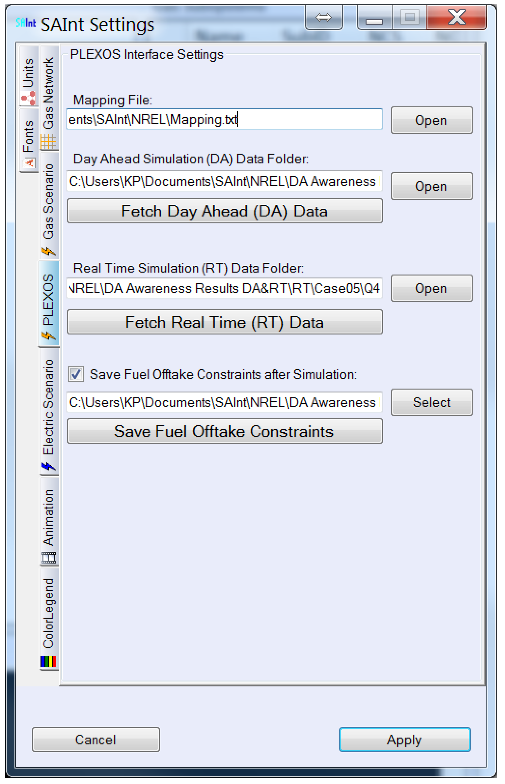
The co-simulation platform is divided into two separate simulators that communicate and exchange data through a co-simulation interface implemented in SAInt, which is depicted in Figure 4.

The interface is responsible for mapping the hourly fuel offtakes of gas generators in the power system model to the corresponding fuel offtake points in the gas model and for transferring the hourly fuel offtake constraints computed by the gas simulator back to the corresponding gas generators in the power system model.

Table 3. Mapping between power system nodes in PLEXOS and gas system nodes in SAInt for the 25 gas fired generators.

PLEXOS Generator ID	SAInt-Node ID
gen04	NO.81
gen06	NO.82
gen08	NO.54
gen10	NO.34
gen13	NO.72
gen16	NO.60
gen19	NO.49
gen22	NO.65
gen23	NO.74
gen25	NO.27
gen28	NO.70
gen29	NO.59
gen30	NO.29
gen33	NO.76
gen36	NO.80
gen37	NO.40
gen39	NO.35
gen43	NO.4
gen44	NO.19
gen47	NO.12
gen48	NO.22
gen50	NO.7
gen51	NO.0
gen53	NO.33
gen54	NO.53

shows how the different gas generator objects in the power system model are mapped with the fuel gas offtake nodes in the gas system.

The hourly fuel offtakes of gas generators computed by PLEXOS are given in the energy units of MMBTU, and correspond to the amount of thermal energy required to generate electric energy for the given hour. This energy requirement is converted to an equivalent gas flow rate in reference conditions by assuming a constant gross calorific value of 38.96 MJ/sm³ for natural gas.

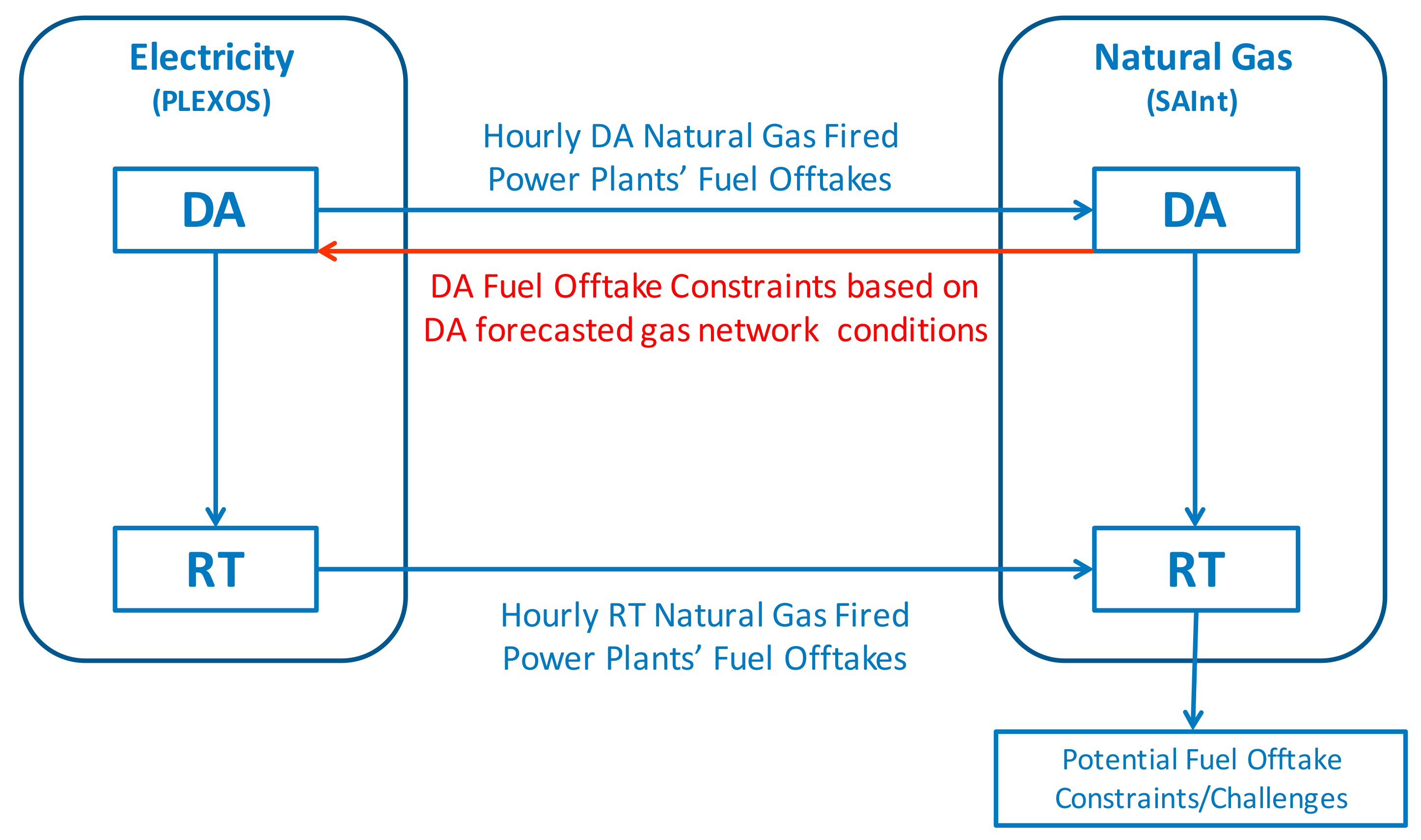
The simulation of the combined energy system is divided into DA and RT simulations as depicted in Figure 5. The DA simulation is first run for the power system and the resulting hourly fuel offtake profiles of gas generators are exported from PLEXOS to SAInt via the co-simulation interface (see, Figure 4) using the mapping information provided in Table 3.

The fuel offtake profiles are then used together with the day-ahead load profiles of other gas customers and the settings of controlled facilities to run a dynamic simulation of the gas system for the day-ahead schedule. To run a dynamic simulation for the gas system, the initial state of the gas system has to be known. To obtain an initial state, we first run a steady state simulation and then use the solution of the steady state as an initial state to run an intermediate dynamic simulation with constant flow profiles, which eventually converges to a steady state condition. The reason for running the intermediate dynamic simulation is to ensure the right settings for all compressor stations and that constraints violated in the steady state are treated by the solver in the intermediate dynamic simulation. The solver does this by changing the control settings of affected facilities (e.g., curtailment of offtakes, if pressure violations are detected in the steady state simulation).

The results of the dynamic gas system simulation include the computed fuel offtake for gas generators, which may differ from the scheduled day-ahead fuel offtake profile computed for gas generators in the power system model if gas curtailments were necessary to respect pressure limits in the gas system. The fuel offtake constraints computed by SAInt can be reported back to PLEXOS to recompute the DA power system simulation, which would generate a new unit commitment schedule for running the real-time power system simulation.

We differentiate between two different cases which differ in terms of how the information about the fuel offtake constraints from the DA gas system simulation are utilized in the power system simulation. We label these situations Business As Usual and DA-Coordination, and they are illustrated in Figure 5 and Figure 6. In the business as usual case depicted in Figure 5, the fuel offtake constraints from the gas system are not utilized by the power system, while in the DA-Coordination case illustrated in Figure 6, the fuel offtake constraints are used to recompute the DA power system simulation. This provides new unit commitment solution for the generators that is then applied in the RT power system simulation.

In both cases, the fuel offtake profiles from the RT power system simulation are provided to the gas system for running a RT gas system simulation using the same procedure as for the DA simulation. The fuel offtake constraints computed for the RT gas system simulation can be sent back to the power system to analyze how the coordination between both systems impacted the operation of the power system.

3. Results

In this section, we present the results of a case study that highlights the differences between coordinating the gas and power systems operation at these time-frames with the current practice of no coordination.

3.1. Scenarios

The scenarios used to showcase the differences are divided into the following:

• Renewable Penetration:
  In terms of level of wind and solar penetration in the generation mix of the power system, we distinguish between three wind and solar penetration levels, 20%, 30%, and 40% in terms of annual electricity generation (as illustrated in Figure 7). Figure 7 shows the share of electricity generation from wind, solar, and natural gas for the four weeks selected for the analysis. The annual penetrations in energy terms of variable renewable energy sources in the three scenarios correspond to 20%, 30% and 40%. The scenarios include higher penetrations of solar power than wind power.

  Table 4. Renewable generation installed capacities in the different renewable penetration scenarios.

  Renewable	Renewable Generation
  Penetration Scenario	Installed Capacity (MW)
  	Solar	Wind
  20%	1114	790
  30%	1770	1015
  40%	2176	1354

  shows the wind and solar power generation capacities for the three renewable penetration scenarios. However, for the four weeks selected, the corresponding wind and solar penetrations do not represent the annual average and are slightly smaller than 20%, 30%, and 40%. The share of electricity generation from natural gas decreases as variable renewable penetration increases because wind and solar power displace electricity generation from natural gas fired generators.
• Season:
  The simulation data for the gas and power system are available for an entire year. However, to highlight the differences between the approaches, we select for each quarter of the year the week with the highest upward-ramp of gas fired generators in the power system. The selection is based on the frequency and magnitude of upward-ramps. We choose to focus on the weeks with highest natural gas offtake ramps as a proxy for weeks that may experience the largest challenges from a natural gas network persperctive. For each wind and solar penetration level, the following weeks were selected for the case studies:

  –

  Q1: From 29 January 2012, 00:00 to 5 February 2012, 12:00 a.m.,

  –

  Q2: From 1 April 2012, 00:00 to 8 April 2012, 12:00 a.m.,

  –

  Q3: From 23 September 2012, 00:00 to 30 September 2012, 12:00 a.m.,

  –

  Q4: From 28 October 2012, 00:00 to 4 November 2012, 12:00 a.m.

• Level of Coordination:
  For each wind and solar penetration level and each selected quarter, two different cases in terms of level of coordination between the gas and power system are investigated, which we denote as follows:

  –

  Business as Usual: Fuel offtake constraints computed from the DA gas system simulation are not considered in the power system simulation. DA and RT power system simulation do not take the fuel offtake constraints of the gas system into account.

  –

  DA-Coordination: Fuel offtake constraints computed from the DA gas system simulation are considered in the power system simulation. The power system recomputes its DA using the fuel offtake constraints and uses the resulting unit commitment schedule for the RT simulation.

The simulation of the gas system requires additional definitions besides the fuel offtake profiles received from the power system additional definitions of control settings with respect to specific conditions in the network. Each simulation in SAInt is modeled as a scenario, which has the following properties:

• Scenario type (steady state, succession of steady steady state, or dynamic simulation).
• Scenario time window (simulation start time and end time).
• Scenario time step (determines the time resolution of the simulation and thus the number of time steps computed).
• Initial State (for a dynamic simulation, an initial state of the gas network is needed).
• Scenario schedule and boundary conditions (includes all control settings and flow schedules for controlled facilities that may change in time. Settings for controlled facilities can be triggered based on certain conditions in the network, e.g., open a valve if the pressure in a region is below a certain value or increases the outlet pressure set point of the compressor if the linepack in a region is below a specific value).

3.1.1. Gas System Control Settings

For all gas system scenarios, we define the following control settings that depend on the conditions in the gas system during the simulation run.

Fuel Offtake Curtailment: For all fuel offtake nodes of gas fired generators, we define a minimum pressure limit of 30 bar-g and for all city gate stations a limit of 16 bar-g. The scheduled offtake at these stations will be curtailed such that the pressure limits at the corresponding node are not violated.

Compressor Operations: Compressor Station CS.5 is used for controlling the pressure in subsystem GSUB.NORTH. If the minimum pressure in GSUB.NORTH goes below 30 bar-g, CS.5 will increase its outlet pressure by 1/15 bar-g/min to restore the pressure level in subsystem GSUB.NORTH, thus reducing risk of potential fuel offtake curtailments of gas generators in that region, which require a minimum fuel gas pressure of 30 bar-g for operation. Increasing the outlet pressure, however, comes with a cost, since the compression of gas requires energy from the driver. Thus, to reduce the energy consumption in times of reduced loads, we define an additional conditional control for CS.5, which reduces the outlet pressure set point by 1/15 bar-g/min if the minimum pressure in GSUB.NORTH is above 32 bar-g.

LNG Terminal Operations: LNG terminal NO.10 has a limited quantity of LNG in its storage tank, which is regasified and injected into the network. If the working inventory of the terminal is depleted, the terminal cannot inject gas into the network and has to shut down, until it is supplied with LNG from a LNG vessel. SAInt is able to model and schedule the arrival of LNG vessels and the discharge of LNG from the vessel to the LNG storage tank by defining the arriving time and size of the LNG vessel and the discharge rate. In all studied scenarios, the arrival of LNG vessels at NO.10 is scheduled every third and sixth day at 6:00 a.m. after the start of the simulation with an arriving vessel size of 40,000 m³ of LNG and a discharge rate of 120 m³/min.

Valve Operations: The shut down of LNG terminal NO.10, due to the depleted working inventory may cause pressure reductions in the surrounding market area, which may eventually lead to curtailments of scheduled fuel offtakes from customers in that area, in particular, GFPPs. To avoid this undesired situation, we define control mode changes for valve station VA.1 that connects subsystem GSUB.SOUTH with GSUB.EAST. If the LNG terminal is not supplying the network with gas (i.e., control mode is OFF) and the minimum pressure in GSUB.EAST is below 30 bar-g, valve station VA.1 should open, while, if the LNG terminal is operating and the minimum pressure in the subsystem is above 32 [bar-g], the station should close in order to reduce the energy consumption of the upstream compressor station.

3.1.2. Gas System Simulation Settings

In addition to the control settings explained above, the simulation parameters and gas properties listed in

Table 5. Input parameter for transient simulation of GNET90 gas network model.

Parameter	Symbol	Value	Unit
time step	$\Delta t$	1800	(s)
total simulation time	$t_{max}$	168	(h)
isothermal gas temperature	T	288.15	(K)
dynamic viscosity	$\eta$	${10}^{-5}$	(kg/m·s)
reference pressure	$p_n$	1.01325	(bar)
reference temperature	$T_n$	288.15	(K)
critical pressure	$p_{crit}$	45	(bar)
critical temperature	$T_{crit}$	193.7	(K)
relative density	d	0.6	-
gross calorific value	$GCV$	38.96	(MJ/sm3)

are applied for all studied scenarios. The time step for the dynamic simulation is set to 30 min; however, the time resolution is adapted by the dynamic time step adaptation method implemented into SAInt if rapid transients occur in the course of the simulation [18].

3.2. Global Results

In the following section, we discuss aggregated results for the computed scenarios, which are illustrated in Figure 8 and Figure 9. Figure 8 compares the total aggregated gas not supplied (GNS) for the four quarters for the three studied wind and solar penetration levels and for the coordination level Business As Usual and DA-Coordination. As can be seen, the GNS for Business As Usual is more than twice as high as for DA-Coordination for all wind and solar penetration levels, which means the coordination between the gas and power system reduced significantly the curtailment of offtakes in the gas system. Furthermore, the level of curtailment of offtake curtailment in the gas system decreases with increasing wind and solar penetration, though one would expect the opposite, since an increased wind & solar penetration level is expected to increase the number of upward and downward ramp cycles, thus affecting pressure limits in the gas system. However, a reason for the observation could be that a higher wind and solar penetration level means less average fuel offtake of gas fired generators, which also means less stress and higher average pressures in the gas system, which in turn makes the gas system less sensitive to potential fuel offtake ramps of gas fired generators to back up wind and solar sources. At higher variable renewable energy penetrations, however, net load ramps are larger and these can cause more frequent natural gas pipeline network constraints on power plants’ natural gas off-take.

The reduced curtailments in the gas system in the DA-Coordination case also positively impacted the total energy consumption of compressor stations in the gas system independent of the wind and solar penetration level, as illustrated in Figure 9. The total energy consumption for the Business As Usual scenario is always roughly 10% higher than in the DA-Coordination case.

3.3. Specific Examples

Below are a few specific examples:

3.3.1. Fuel Offtake Curtailment

Figure 10 shows an example of fuel offtake curtailment at node NO.80 of gas generator gen36 for the DA gas system simulation for Q1 and for a 20% renewable penetration level. The top plot shows the time evolution of the nodal pressure, the middle plot compares the time evolution of the scheduled offtake profile (i.e., profile received from the results for the DA power system simulation in PLEXOS) to the actual offtake profile (i.e., offtake profile computed by the DA gas system simulation in SAInt considering the operation and pressure limits in the gas system) and the bottom plot is the cumulative quantity of gas not supplied from the start of the simulation (i.e., the integral of the area between the green (scheduled offtake, NO.80.QSET) an blue curve (actual offtake, NO.80.Q) in the middle plot). As can be seen, the scheduled offtake is curtailed whenever the pressure in node NO.80 reaches the pressure limit of 30 bar-g.

3.3.2. Compressor Operations

The conditional control prescribed to compressor station CS.5 is illustrated in Figure 11 for the DA gas system simulation for Q1 and for a 20% renewable penetration level. The top plot shows the time evolution of the minimum pressure in subsystem GSUB.NORTH, while the center and bottom plot show the time evolution of the outlet pressure and the driver power for compressor station CS.5, respectively. As can be seen, the outlet pressure of the compressor station increases linearly if the minimum pressure in GSUB.NORTH decreases below 30 bar-g and decreases linearly if the minimum pressure in GSUB.NORTH increases above 32 bar-g. Furthermore, the energy consumption of the compressor station increases if the outlet pressure increases and decreases if the outlet pressure decreases.

3.3.3. LNG Terminal Operations

The top left plot in Figure 12 shows the time plot for the working inventory of LNG terminal NO. 10 for the DA gas system simulation for Q1 and for a 20% renewable penetration level. The inventory decreases almost linearly right from the start of the simulation until the working inventory is depleted, which causes the station to stop its gas supply to the network as can be seen in the bottom left and right plot in Figure 12, where the time evolution of the control mode and gas supply are plotted. The terminal resumes its gas supply after the arrival of the first vessel on 1 February, at 6:00 a.m. The LNG transported by the vessel is discharged and relocated to the storage tanks in the terminal as can be seen in the increasing working inventory after the arrival of the vessel. The discharge process takes approximately 5.5 h, and then the inventory starts decreasing again until the second vessel arrives.

3.3.4. Valve Operation

Figure 13 shows how the conditional control setting for valve station VA.1 is respected in the simulation for the DA gas system simulation for Q1 and for a 20% renewable penetration level, where the minimum pressure in subsystem GSUB.EAST and the control and flow rate of valve station VA.1 is plotted over time. As can be seen, the valve station is opened (i.e., control mode BP) and supplies gas to GSUB.EAST if the minimum pressure in the subsystem is below the defined pressure threshold.

4. Conclusions

In this paper, we developed a co-simulation platform to assess the operation and interdependence between natural gas and power transmission networks. The platform consists of a steady state DC unit commitment and economic dispatch model to simulate bulk power system operations and a transient model to simulate the operation of bulk natural gas pipeline networks. The models are implemented in two separate simulation environments, namely, PLEXOS [14], a production cost modeling tool for electric power systems and SAInt [15], a transient hydraulic gas system simulator. The data exchange and communication between both simulation environments are established by an interface that maps the power generation of gas generators in the power system to the corresponding fuel offtake points in the gas system.

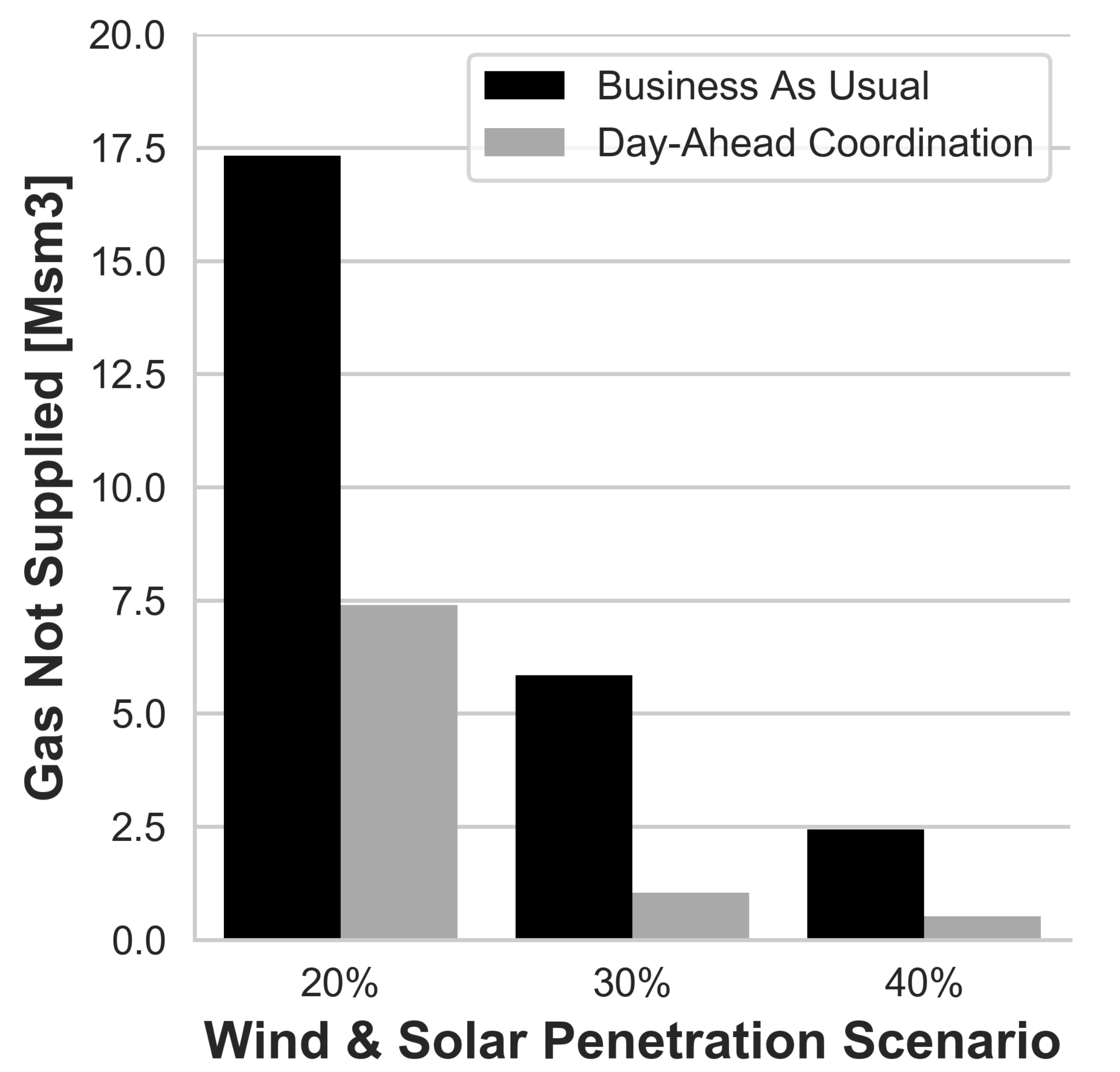
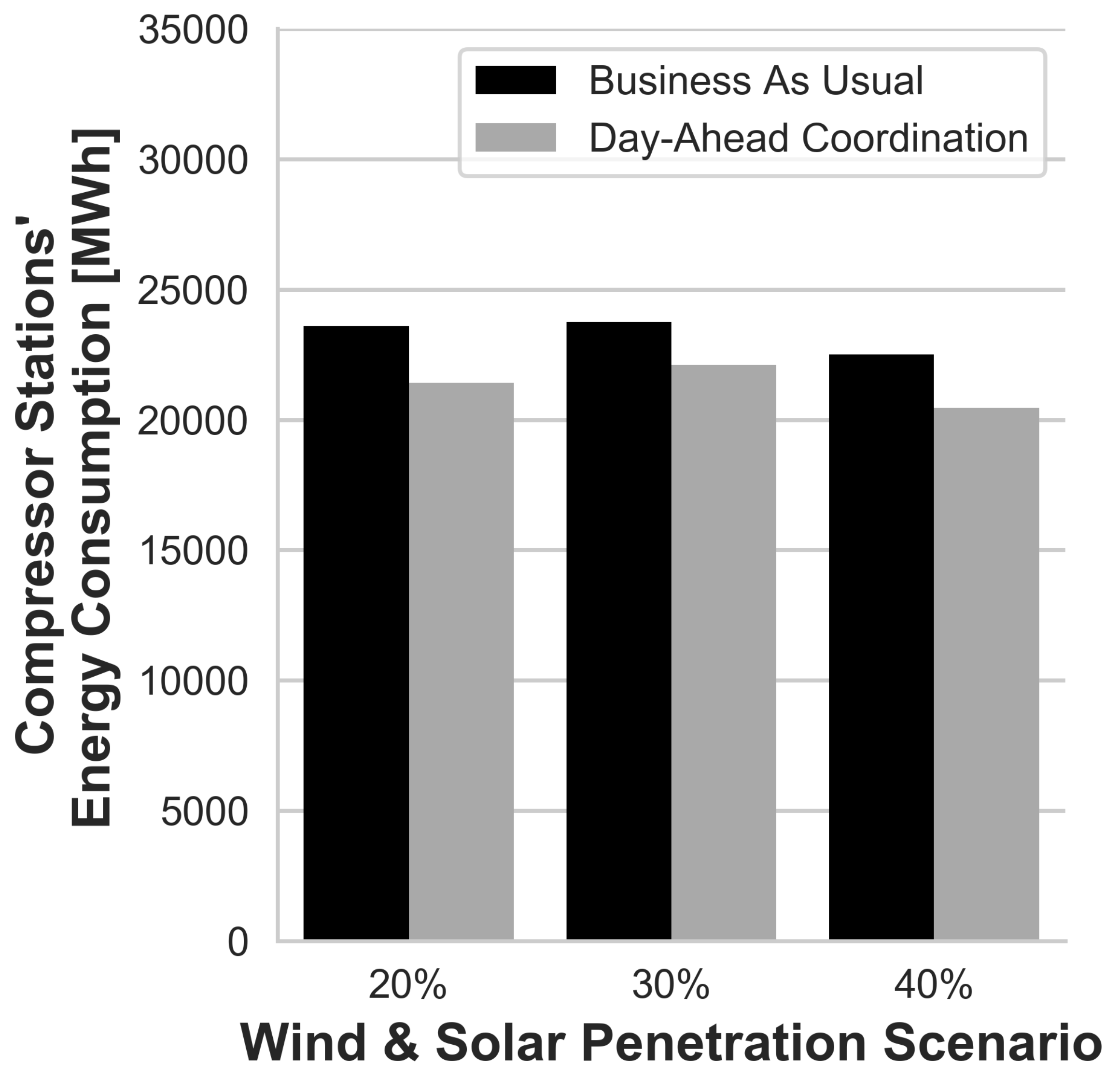
The co-simulation platform was applied on a case study on an interconnected gas and power transmission network test system with the objective to examine to what extent the day-ahead coordination between gas and power TSOs may impact the efficiency and reliability of the coupled energy systems. The two networks are interconnected at 25 gas fired power plants, which represent generation units in the power system and gas offtake points in the gas system. The case study was divided into three dimensions, namely, the level of renewable penetration, the the time period under consideration with the highest upward and downward ramp of gas generators, and, finally, the level of coordination between the gas and power system networks (day-ahead coordination and no coordination between both energy networks). The results from the case study indicate that day-ahead coordination between gas and power system networks contributes to a significant reduction in curtailed gas during high stress periods (e.g., large gas offtake ramps) and up to a 9% reduction in gas consumption at gas compressor stations, for the combined test system examined here. This has implications for real natural gas and power systems where such significant reductions in natural gas curtailment and natural gas compression energy consumption reductions would lead to significant economic and reliability benefits to the both the natural gas and power systems.

In the future, we intend to extend the co-simulation platform by a quasi-dynamic real-time simulation of gas and power systems operation, which will enable the assessment of the impact of real-time coordination and regulatory constraints on the efficiency and reliability of coupled gas and power system networks. We also intend to analyse scenarios with higher penetration of renewable generation.