Optimization Strategy for Economic Power Dispatch Utilizing Retired EV Batteries as Flexible Loads

Abstract

With the increasing penetration of new and renewable energy, incorporating variable adjustable power elements on the demand side is of particular interest. The utilization of batteries as flexible loads is a hot research topic. Lithium-ion batteries are key components in electric vehicles (EVs) in terms of capital cost, mass and size. They are retired after around 5 years of service, but still retain up to 80% of their nominal capacity. Disposal of waste batteries will become a significant issue for the automotive industry in the years to come. This work proposes the use of the second life of these batteries as flexible loads to participate in the economic power dispatch. The characteristics of second life batteries (SLBs) are varied and diverse, requiring a new optimization strategy for power dispatch at the system level. In this work, SLBs are characterized and their operating curves are obtained analytically for developing an economic power dispatch model involving wind farms and second life batteries. In addition, a dispatch strategy is developed to reduce the dispatch complex brought by the disperse spatial and time distribution of EVs and decrease the system operating cost by introducing incentive and penalty costs in regulating the EV performance. In theory, SLBs are utilized to reduce the peak-valley difference of power loads and to stabilize the power system. Test results based on a ten-unit power system have verified the effectiveness of the proposed dispatch model and the economic benefit of utilizing SLBs as flexible loads in power systems. This work may provide a viable solution to the disposal of waste batteries from EVs and to the stable operation of fluctuating power systems incorporating stochastic renewable energy.

1. Introduction

Modern power networks contain a high proportion of new and renewable energy sources such as wind, solar, bioenergy and so forth. They are characterized by intermittence, which gives rise to uncertainty on the supply side. In practice, a continuous and stable power supply is highly desired for economic power dispatch. In this regard, sufficient reserve power from thermal generators and energy storage devices is always utilized in order to accommodate the stochastic new and renewable energy in traditional power dispatch [1,2]. With the rapid development of the electricity market on the user side, the effective power balance requires extensive use of dispatchable flexible loads, which is a significant current research focus.

Flexible loads are the loads with flexible features which can give an initial response to power system dynamics [3]. They can play an important role in peak-load shaving of power systems by decreasing load fluctuations. In turn, they can increase the penetration of new and renewable energy in the power system [4]. Flexible loads can be traditional industrial, commercial and resident loads used in a controllable manner [5]. Bidirectional dispatchable loads such as energy storage systens [6,7,8] and electric vehicles (EVs) can also be utilized as flexible loads to participate in power dispatch [9,10].

The number of EVs has rapidly increased in the past five years across the world. It is estimated that their penetration will reach 50% by 2020 [11]. The large amount of EVs connected to power grids will create challenges as well as a means of bidirectional dispatchable energy source for power dispatch. EVs can response to the power system on the load side through charging management schemes and thus decrease the fluctuation of power systems [12]. In general, the charging service fee and time-of-use tariff are used to manage the EV charging events, and the economy can be optimized [13,14]. However, the dispersing spatial and time distribution of EVs will also make the power dispatch more complex. During the power dispatch considering EVs as flexible loads, the policy incentives and penalty charges are accounted for to shift the charging time, power and location of EVs. Thus the operating cost of the system will be increased. In addition, the EV user satisfaction is also a key element in the power dispatch, placing more constraints on the optimization of power dispatch. As a result, this paper proposes the use of SLBs in the economic power dispatch in place of EVs.

Batteries with 70% to 80% of their rated capacity are considered to be less useful in EVs and are typically removed from applications at around five years of use [15]. Moreover, these retired batteries are costly to dispose of and the recycling rate of retired batteries is less than 2% [16]. This will cause environmental pollution and a waste of natural resources. Reusing these retired batteries after their first life is economically feasible and can maximize their charging and discharging values. In this way, the “second life batteries” (SLBs) can be utilized in power systems as new flexible loads and they are thus termed the “second life battery flexible loads” (SLBFLs). They can provide the reliable electrical energy when needed, and can response to the demand quickly and flexibly (compared to conventional generating sets) [17].

In the literature, there are some studies reported on the detailed characterization of SLBs, such as the estimation of the state of charge (SoC), state of health (SoH) and depth of discharge (DoD) [18,19]. Reference [20] investigates the future availability of end-of-life EV batteries and their potential use as energy storage. The characteristics of SLBs and their utilization at the level of a domestic dwelling are studied in [21]. Reference [22] describes a methodology to analyze the SLB performance and degradation based on the first life battery ageing data. These studies focus on the detailed characteristics of SLBs while there are few studies on the relationship of SoC and power output of SLBs from a power dispatch perspective. An EV battery charging and discharging performance management method is studied in a macro environment in [9]. Moreover, a detailed economic analysis of SLBs is conducted according to the EV policy incentives [10]. In some studies, EVs are used as battery energy storage systems [23,24,25,26,27] to support the weak grid, which is termed the vehicle-to-grid (V2G), where the batteries are still in the EVs [28]. A cloud-connected battery management approach for decision making on vehicle battery second-life was introduced in [29], in which the residual value of vehicle batteries with respect to various potential SLB applications is estimated. These studied the batteries retired from EVs and reutilization in low-power applications. Reference [30] provides a novel scheme to optimize the number of EV charging stations with the energy storage support of SLBs. In this case, the SLBs are reused in the EV charging station and connected to the power grid. But the relationship of SoC and power output is estimated by a linear approximation which does not reflect the actual characteristic of SLBs.

In the literature, however, there is no reported work on the utilization of SLBs in power dispatch as flexible loads at MW levels. In theory, SLBs can be connected to the supply side as a “power generator” or the load side as a “flexible load”, but the former has higher voltage quality and stability requirements than the latter. Furthermore, the lower voltage grade on the load side requires fewer batteries to be connected to the grid, so as to ensure the safety and stability of the battery packs [31,32]. The characteristics of SLBs have changed after their first life in the EVs and their performance datasheets from original manufacturers are no longer valid for analyzing their second life operation [28]. Thus, new functions for battery management system (BMS) [33,34] are needed to measure individual cells and manage the performance of the SLBs.

In this paper, an economic power dispatch with SLBs as flexible loads is proposed, with a focus on the improvement of the dynamic response and reduction of fluctuations of thermal generators caused by the stochastic wind power in the system. A simulation model based on a ten-unit power system is developed and tested in MATLAB (R2018a, MathWorks, Natick, Massachusetts, USA). The operating characteristics of SLBs are monitored and fed into the system control dynamically; the SLBs are also compared with EVs used as flexible loads for power dispatch purposes. The contributions of this work are as follows:

(i)

A stochastic day-ahead economic power dispatch model with wind farms and SLBFLs at MW levels is developed. This model utilizes batteries retired from EVs as flexible loads for balancing power and also for minimizing the operating cost and environmental emissions.

(ii)

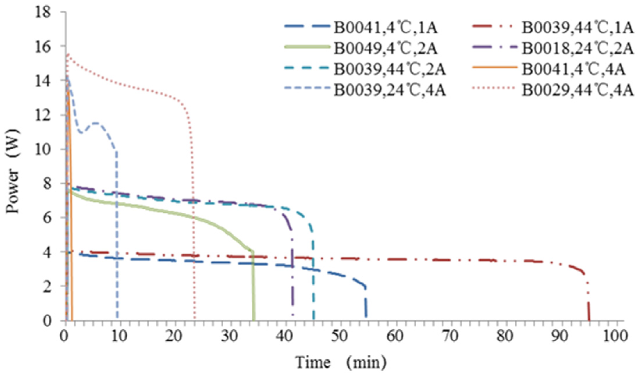
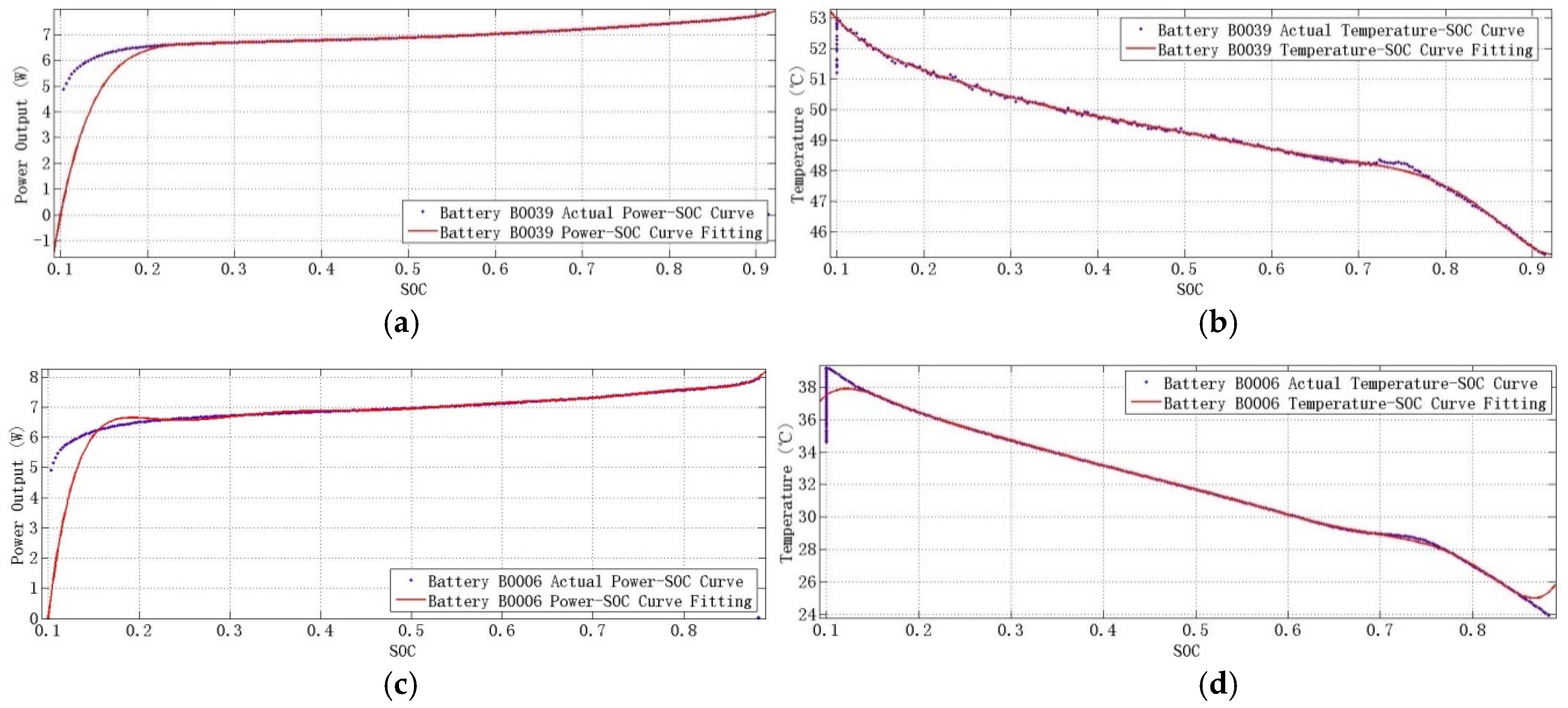
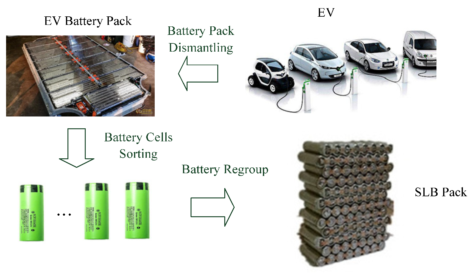
The charging and discharging characteristics of SLBs at different temperatures and currents are obtained and analyzed based on actual NASA battery data.

(iii)

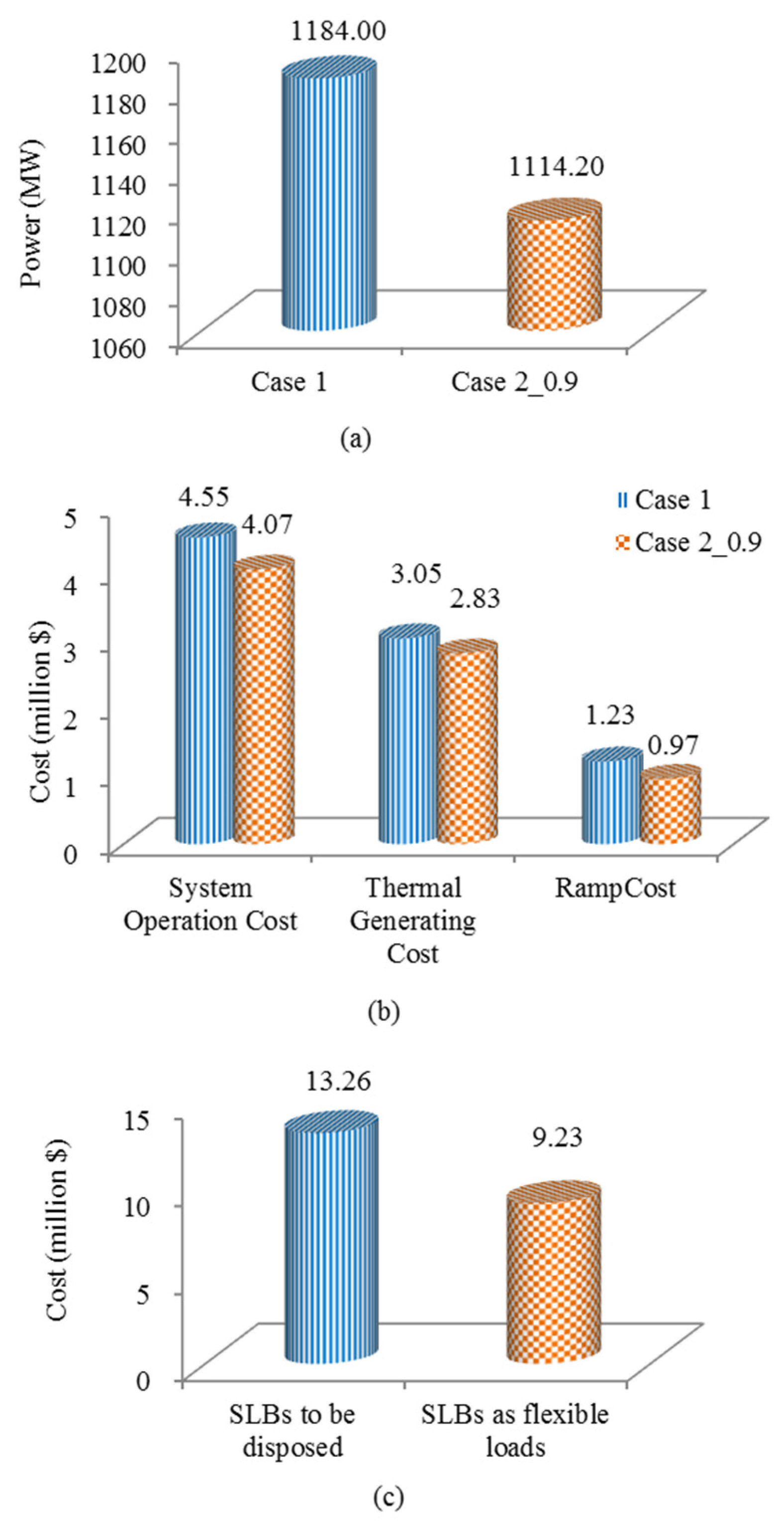
The opportunity cost is calculated to compare between the reuse and the disposal of SLBs; an economic analysis is carried out to compare the utilization of SLBs and EV first-life batteries as flexible loads; the thermal power generating cost and the peak-valley difference of loads are also compared with the system involving SLBs in the power dispatch.

(iv)

This work has proved that SLBs are more economical to be utilized in large quantity for power dispatch. This will have significant economic implications and environmental benefits for both automotive industry and power industry.

2. Second Life Batteries Characteristics Analysis

The battery characteristics provide key information about the battery performance during the charging and discharging periods. This is particularly true for SLBs. The relationships of their SoC, power capacity, charging/discharging currents and battery temperatures are complex and need proper analysis before participating in the power dispatch.

2.1. Battery Power Output under Different Operating Temperatures and Charging/Discharging Currents

In order to analyze the effect of temperature and current on the SLB performance, a pack of lithium-ion batteries (Type 18650, rated capacity of 2 Ahr, from NASA, Washington, DC, USA) are chosen and analyzed by using their tested charging and discharging data at the operating temperature of 4 °C, 24 °C and 44 °C, respectively. Firstly, charging is carried out in a constant current (CC) mode at 1.5 A until the battery voltage reaches 4.2 V, followed by the charging in a constant voltage (CV) mode until the battery current drops to 20 mA. Then, discharging is carried out in a constant mode at 1 A, 2 A and 4 A for different groups of batteries until the terminal voltage falls to a given value (2.0 V, 2.2 V and 2.7 V). The tests are performed repeatedly until the battery capacity reduces to 1.4 Ahr, which is 70% of the rated capacity [35]. This degradation is mainly caused by cell oxidation and internal material corrosion mechanism [36] and will continue to deteriorate with the service cycle. In order to make the difference between SLBs and new batteries, all the SLB battery data (e.g., battery capacity, discharging current, discharging voltage and temperature) are obtained from NASA where the batteries’ remaining capacity is 80% of the rated and below.

The battery discharging characteristics at different temperatures and currents are plotted in Figure 1. It can be seen that the batteries discharging at 4 A will achieve a higher power output than those at 2 A and 1 A. However, all the power outputs of batteries dropped quickly within 30 min, and the one at 44 °C can last the longest time. All the batteries discharging at 2 A and 1 A have a steady discharging period. The higher power output the battery has, the less batteries are needed in the battery pack. In a day-ahead power dispatch, the dispatch time scale is set at 15 min, and thus the operational time of the SLB pack needs to be at least 15 min. The SLB pack only meets this requirement at the discharging current of 1 A and 2 A. Thus, the rated current (i.e., 2 A) is chosen in this case. According to Figure 1, the discharging time is the longest at the temperature of 44 °C. Therefore, the SLB operating temperature is set at 44 °C to achieve a long discharging time. Under a BMS balance control, the output power of battery cells is 8 W (at 2 A and 44 °C).

Figure 2 shows the actual operational characteristics of SLBs as a function of their SoC (NASA Batteries B0006 and B0039). The capacity-SoC curve is used to provide the power output capability of the SLBs and the temperature-SOC to show the temperature limits of SLBs. The operational temperature is critically important for battery operation and it influences on the internal resistance of SLBs. As the SoC decreases, the battery capacity reduces and the temperature increases. The changing tendency of the curve is conformed to the battery charging/discharging characteristics. It can also be seen that the temperature-SoC and capacity-SoC curves are not linear. As a result, accurate measurement data are needed for the BMS before the SLBs are connected to the power grid for power dispatch. In this work, accurate charging and discharging data of SLBs are obtained through curve fitting by using the MATLAB tool boxes.

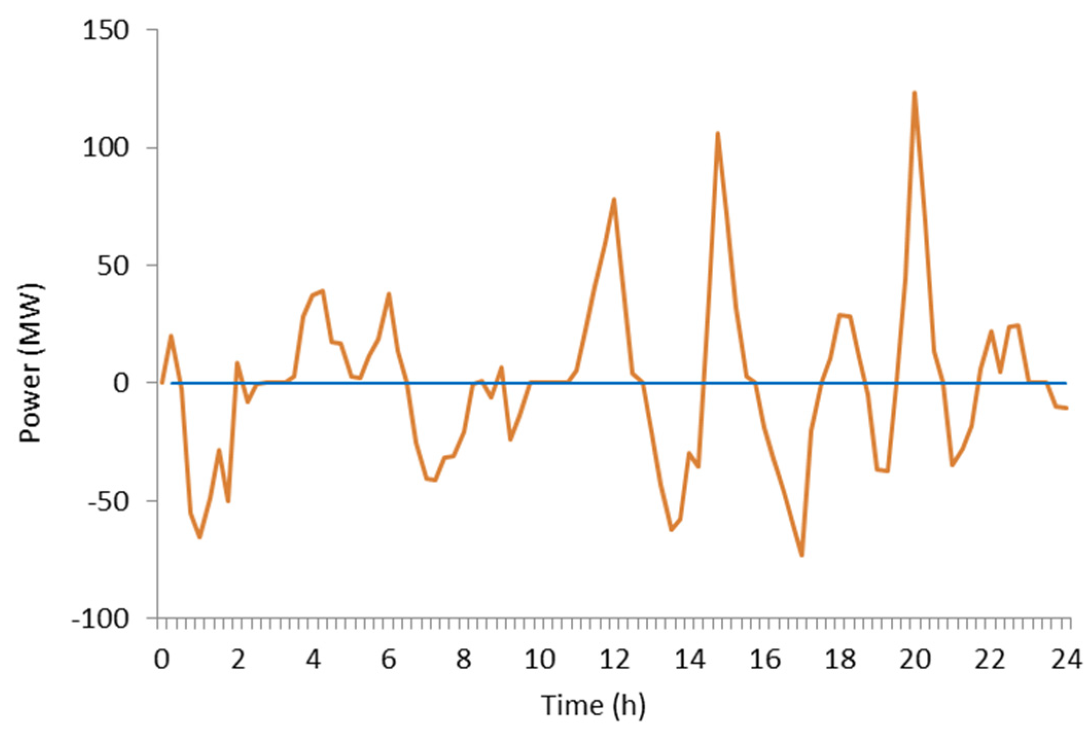
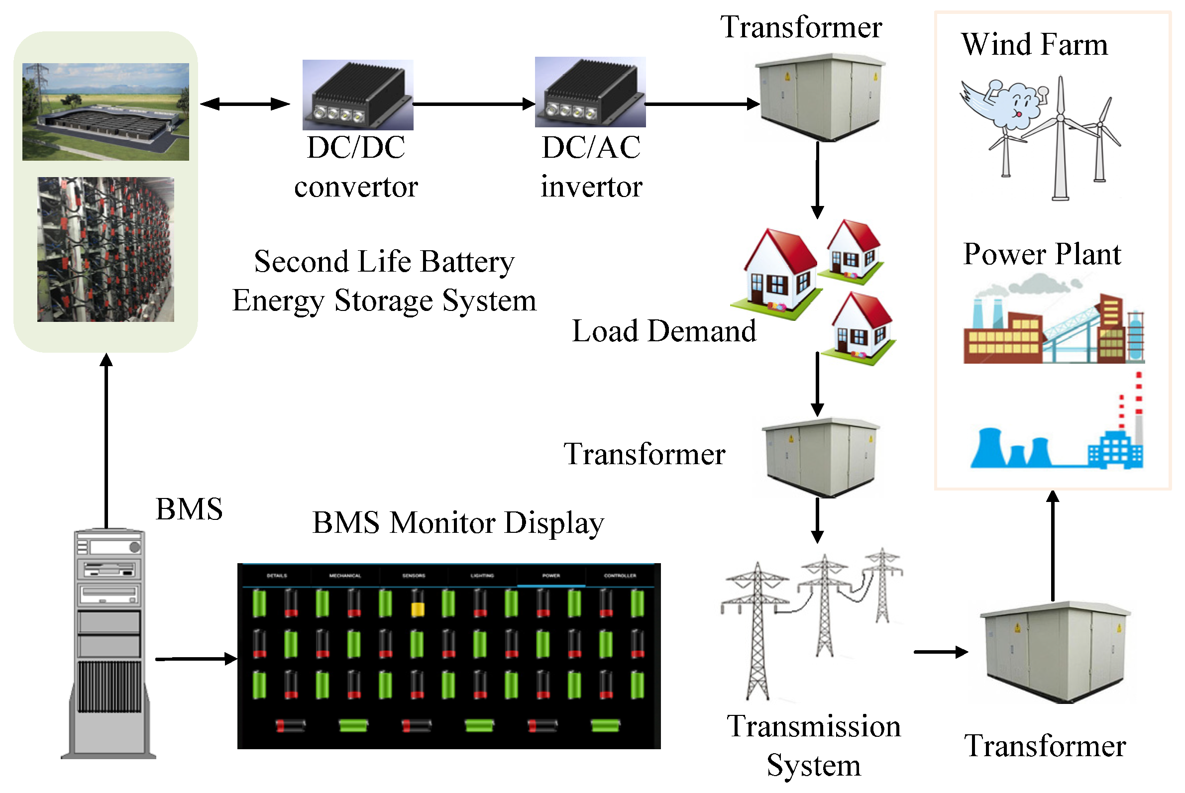
2.2. SLBFLs in Power Dispatch

The producing process of SLB pack is shown in Figure 3, and the batteries retired from EVs are regrouped to form a new SLB pack. The SLB pack is composed of several battery units which are connected in parallel to increase the output current and in series to increase the output voltage. In one battery unit, there are hundreds of battery cells connected in parallel, because Lithium-ion batteries tend to be open-circuited when faulted and the parallel connection will reduce the impact of the faults. Battery cells connected in parallel can increase the unit capacity, and a SLB pack with many battery units can be regarded as flexible loads when connected into the power network.

Figure 4 shows a schematic diagram of the proposed power grid incorporating SLBs and wind farms. The system consists of a power plant, a SLB pack and a BMS, wind farms, transformers, power converters and transmission lines. The BMS can measure the cell temperatures, and estimate the SoC and SoH. It is used to control the overall functionality of the battery, balancing tasks and charging and discharging processes. The DC/DC converter is employed to increase the battery voltage and the DC/AC converter is utilized to converter a fixed DC voltage into an AC voltage. Transformers are employed to match the voltage level between the converter output and the grid.

3. Economic Power Dispatch Model with Wind Farms and SLBFLs

In this section, a day-ahead economic power dispatch with SLBFLs is provided. The traditional optimization problem contains an objective function, some balance constraints, and variable limits. Normally, the economic dispatch problem can be formulated as:

$$\{\begin{array}{ll}\min & f(x)\\ s.t.& g(x)=0\\ & \underset{\_}{h}(x)\le h(x)\le \overline{h}(x)\end{array}$$

(1)

where $f(x)$ is the objective function;

• $g(x)$ is the balance constraint;
• $h(x)$ is the unequal constraint;
• $\underset{\_}{h}(x)$ is the minimum value of the unequal constraint;
• $\overline{h}(x)$ is the maximum value of the unequal constraint.

3.1. Objective Functions

The thermal generation cost $F_{thermal}$, environmental emissions cost $F_{pollution}$, spinning reserve cost $F_{reserve}$ and generators ramp cost $F_{ramp}$ are considered in this paper. In the model, a ripple effect (when the turbine inlet valve is suddenly opened) is needed to take into account. This is done by a curve superposition technique. In addition, the valve-point loading effect [37] is also considered in deriving the fuel cost function of each unit. This is calculated by:

$$F_1=F_{thermal}={\displaystyle \sum _{t=1}^T{\displaystyle \sum _i^n\{a_{pi}\times P_{i,t}^2+b_{pi}\times P_{i,t}+c_{pi}+\left|e_{pi}\sin \left[f_{pi}(P_i^{\min }-P_{i,t})\right]\right|\}}}$$

(2)

where T is the number of hours in operation; n is the number of dispatchable units; $a_{pi}$, $b_{pi}$, $c_{pi}$, $e_{pi}$ and $f_{pi}$ are the coefficients of fuel cost functions for units i; $P_{i,t}$ is the real power output.

There is an absolute value in the fuel cost objective function, which can be built up by a piecewise function. But this also needs a smoothing process through an aggregate function method [38]. This objective function is given by:

$$F_{fuel}={\displaystyle \sum _{t=1}^T{\displaystyle \sum _{i=1}^n\{a_{pi}\times P_{i,t}^2+b_{pi}\times P_{i,t}+c_{pi}}}+\frac{1}{p}\ln (e^{p\left\{e_{pi}\sin \left[f_{pi}(P_i^{\min }-P_{i,t})\right]\right\}}+e^{p\left\{-e_{pi}\sin \left[f_{pi}(P_i^{\min }-P_{i,t})\right]\right\}})\}$$

(3)

The objective function after the smoothing process is continuous and differentiable, and then it is applied to general optimization methods.

The environmental emissions cost is calculated on the basis of CO₂ emissions, which is shown in Equation (4):

$$F_2=F_{pollution}={\displaystyle \sum _{t=1}^T{\displaystyle \sum _i^n(a_{ci}\times P_{i,t}^2+b_{ci}\times P_{i,t}+c_{ci})}}$$

(4)

where $a_{ci}$, $b_{ci}$, and $c_{ci}$ are the coefficients of environmental emissions cost functions for unit i.

In this regard, the costs of wind farms are considered as the spinning reserve arising from the difference between the predicted wind power and the actual wind power. That is:

$$F_{UR}={\displaystyle \sum _{i=1}^n(Co{e}_{URi}\times {\displaystyle \sum _{t=1}^T{P}_{URi,t}})}$$

(5)

$$F_{DR}={\displaystyle \sum _{i=1}^n(Co{e}_{DRi}\times {\displaystyle \sum _{t=1}^T{P}_{DRi,t}})}$$

(6)

$$F_3=F_{reserve}=F_{UR}+F_{DR}$$

(7)

where $P_{URi,t}$ is the actual up-reserve of ith generator at time t and $P_{DRi,t}$ is the actual down-reserve of ith generator at time t. $F_{UR}$ and $F_{DR}$ are the up-spinning reserve cost and down-spinning reserve cost, respectively; $Co{e}_{URi}$ and $Co{e}_{DRi}$ are the wind power insufficient and surplus cost coefficient of the ith wind farm, respectively.

In addition to the operating cost, the ramp-up and ramp-down costs of thermal generators should be considered in actual power system operating periods. Related functions are given in Equations (8) and (9):

$$F_{ramp-up}={\displaystyle \sum _{i=1}^n[Co{e}_{ramp-upi}\times {\displaystyle \sum _{t=1}^T\max (P_{i,t}-P_{i,t-1},0)}]}$$

(8)

$$F_{ramp-down}={\displaystyle \sum _{i=1}^n[Co{e}_{ramp-downi}\times {\displaystyle \sum _{t=1}^T\max (P_{i,t-1}-P_{i,t},0)}]}$$

(9)

$$F_4=F_{ramp}=F_{ramp-up}+F_{ramp-down}$$

(10)

where $F_{ramp-up}$ and $F_{ramp-down}$ are the ramp-up cost and ramp-down cost of thermal generators, respectively; $Co{e}_{ramp-upi}$ and $Co{e}_{ramp-downi}$ are the ramp-up cost and ramp-down cost coefficients of the ith thermal generator, respectively.

The opportunity cost (OC), also known as the alternative cost, is the best value of a loss opportunity in a decision making process. In the electrical energy market, the OC is regarded as the profit compensation that it would have made if making other choices instead of the current one [39]. The OC of SLBs as flexible loads is the best profit of the batteries to be recycled as metal materials (described as $F_{OCFL}$). The OC of SLBs to be recycled is the best profit of batteries as flexible loads, which provides the cost-saving from the developed system. In this paper, it is equal to the maximum cost of the same battery power outputs from the thermal plants.

In order to speed up the decision making, a technique of approximate order preference is employed [40] to deal with the objective function:

$$f_j=\left|\frac{F_j-F_j^{\ast }}{F_j^{\ast }}\right|$$

(11)

$$F={\displaystyle \sum _{j=1}^4{f}_j}$$

(12)

where $F_j$ is the jth objective function and $F_j^{\ast }$ is the optimized solution to $F_j$ under the single object function optimization. $f_j$ is the normalized objective function. Its minimum value is 0, indicating that the result is the closest to the optimized solution.

3.2. Constraint Functions

The power balance equations at time t are formulated as:

$$P_{Generationt}={\displaystyle \sum _{i=1}^n{P}_{i,t}}+{\displaystyle \sum _{i=1}^{nw}{P}_{w{p}_{i,t}}^{pre}}$$

(13)

$$P_{Loadt}=P_{slb,t}+P_{Dt}$$

(14)

$$P_{Generationt}-P_{Loadt}=0$$

(15)

where $P_{Generationt}$ and $P_{Loadt}$ are the total power generation and the total load demand at time t, respectively. ${\displaystyle \sum _{i=1}^n{P}_{i,t}}$ is the total generator power output during the tth time period. $P_{wpi,t}^{pre}$ is the predicted wind power of wind farm i at time t. ${\displaystyle \sum _{i=1}^n{P}_{wpi,t}^{pre}}$ is the total predicted wind power output at time t. $P_{slb,t}$ is the SLB power output at time t. If it is positive, the SLBs is charged by the power grid. If negative, the SLBs are discharging power to the grid. $P_{Dt}$ is the total load demand during the tth time period:

$$P_i^{\min }\le P_{i,t}\le P_i^{\max }$$

(16)

where $P_i^{\min }$ and $P_i^{\max }$ are the minimum and maximum power outputs of the ith thermal generator, respectively.

The generating unit ramp rate limits are formulated by:

$$\{\begin{array}{l}{P}_{i,t}-P_{i,t-1}\le U{R}_i\\ P_{i,t-1}-P_{i,t}\le D{R}_i\end{array}$$

(17)

where $U{R}_i$ and $D{R}_i$ are the ramp-up and ramp-down rate limits of the ith thermal generator, respectively.

The SLBFLs constraints are given by:

$$SO{C}^{\min }\le SO{C}_t\le SO{C}^{\max }$$

(18)

$$T_{slb,t}=k({\mathrm{SOC}}_t)$$

(19)

$$T_{slb,t}\le T_{slb}^{\max }$$

(20)

$$E_0=E_T$$

(21)

$$P_{slb,t}=(E_{capacity,t}-E_{capacity,t-1})/\Delta t$$

(22)

$$E_{capacity,t}=g({\mathrm{SOC}}_t)$$

(23)

where $SO{C}_t$ is the state of charge of the SLB at time t. $SO{C}^{\min }$ and $SO{C}^{\max }$ are the minimum and maximum SoC of SLB, respectively. $E_0$ and $E_T$ are the SLB capacity at the initial state and the final state, respectively. $E_{capacity,t}$ is the SLB power capacity at time t. $g({\mathrm{SOC}}_t)$ is the relationship between $E_{capacity,t}$ and $SO{C}_t$. This is derived from the NASA experiments and SoC curve fitting introduced in Section 2.

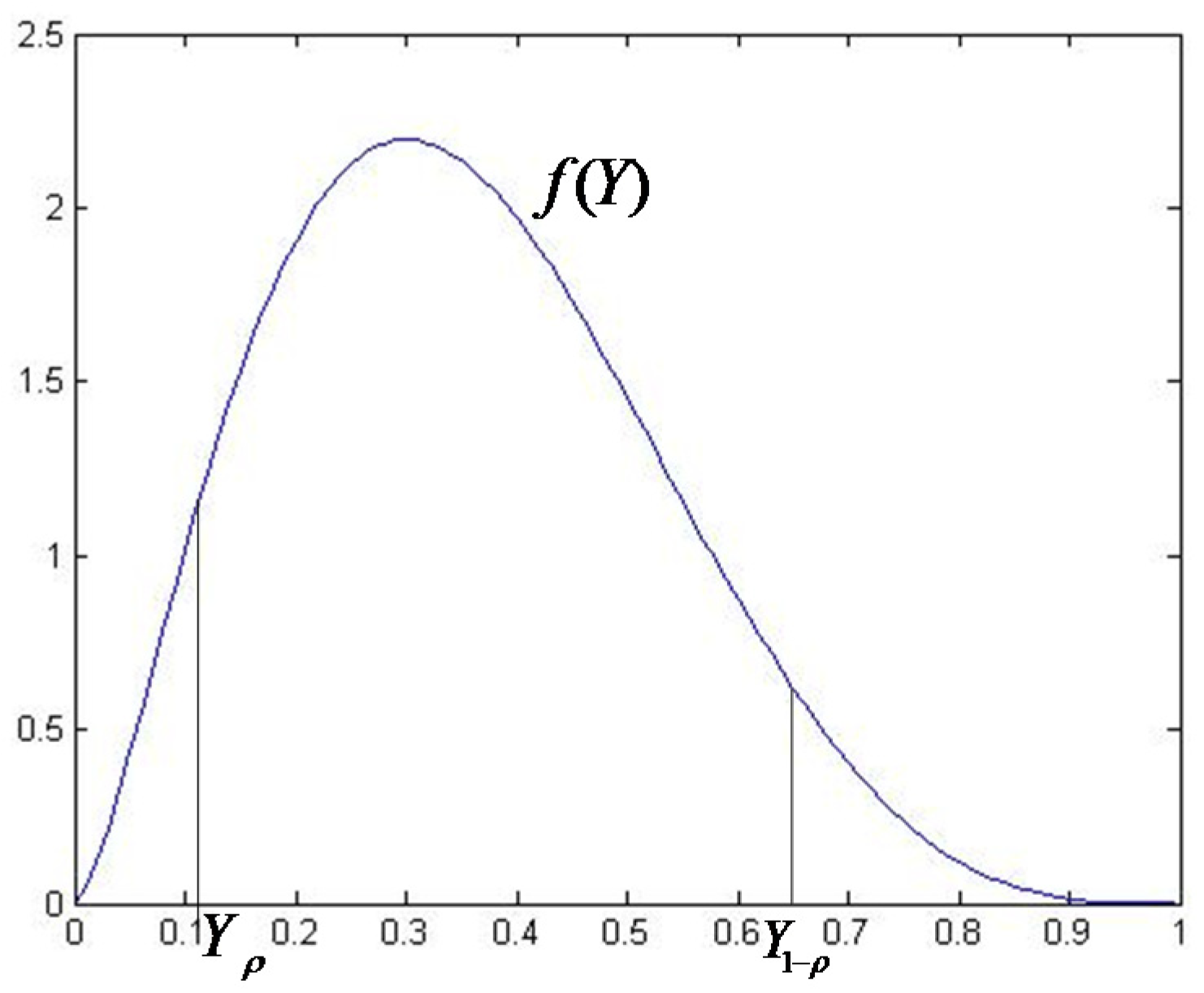
3.3. Stochastic Variables

In general, the wind power output is estimated based on the Beta distribution which represents the probability distribution of wind power for a given site [41,42]. This is shown in Figure 5 and described by:

$$f_w(p_{wp})=\frac{p_{wp}^{\alpha -1}{(1-p_{wp}^{})}^{\beta -1}}{B(\alpha ,\beta )}$$

(24)

where $p_{wp}$ is a normalized wind power output, $B(\alpha ,\beta )$ is the Beta distribution function and $\alpha ,\beta$ are the distribution shape parameters:

$$p_{wp}=\frac{P_{wp}-P_{wp}^{\min }}{P_{wp}^{\max }-P_{wp}^{\min }},p_{wp}\in [0,1]$$

(25)

$$B(\alpha ,\beta )={{\displaystyle {\int }_0^1{p}_{wp}^{\alpha -1}\times (1-p_{wp})}}^{\beta -1}\mathrm{d}{p}_{wp}$$

(26)

$$E(p_{wp}^{pre})=E(\frac{P_{wp}^{pre}}{P_{wp}^{\max }})=\frac{\alpha }{\alpha +\beta }$$

(27)

$$D(p_{wp}^{pre})=D(\frac{P_{wp}^{pre}}{P_{wp}^{\max }})=\frac{\alpha \beta }{{(\alpha +\beta )}^2(\alpha +\beta +1)}$$

(28)

where $P_{wp}$ is the actual wind power output; $P_{wp}^{\min }$ and $P_{wp}^{\max }$ are the minimum and maximum outputs of wind turbines, respectively. $P_{wp}^{pre}$ is the predicted wind power; $E(p_{wp}^{pre})$ is the expectation of $P_{wp}^{pre}$; and $D(p_{wp}^{pre})$ is the variance of $P_{wp}^{pre}$.

The spinning reserve chance constraints are formulated by:

$$\mathrm{Pr}\left\{{\displaystyle \sum _{i=1}^n\left[\min \left(P_i^{\max }-P_{i,t}^{},U{R}_i\right)\right]}\ge {\displaystyle \sum _{i=1}^{nw}(P_{wpi,t}^{pre}-P_{wpi,t}^{})}\right\}\ge \rho$$

(29)

$$\mathrm{Pr}\left\{{\displaystyle \sum _{i=1}^n\left[\min \left(P_{i,t}^{}-P_i^{\min },D{R}_i\right)\right]}\ge {\displaystyle \sum _{i=1}^{nw}(P_{wpi,t}^{}-P_{wpi,t}^{pre})}\right\}\ge \rho$$

(30)

$${\displaystyle \sum _{i=1}^n{P}_{URi,t}={\displaystyle \sum _i^{nw}\max \left[(P_{wpi,t}^{pre}-P_{wpi,t}^{}),0\right]}}$$

(31)

$${\displaystyle \sum _{i=1}^n{P}_{DRi,t}={\displaystyle \sum _i^{nw}\max \left[(P_{wpi,t}^{}-P_{wpi,t}^{pre}),0\right]}}$$

(32)

$$P_{URi,t}\le \min \left(P_i^{\max }-P_{i,t}^{},U{R}_i\right)$$

(33)

$$P_{DRi,t}\le \min \left(P_{i,t}^{}-P_i^{\min },D{R}_i\right)$$

(34)

where $\rho$ is the confidence coefficient and $P_{wpi,t}$ is the actual wind power of wind farm i at time t.

The fractile is used to solve the above chance constraints [43]:

$$\mathrm{Pr}\left(Y>Y_{\rho }\right)=\rho \rho \in \left(0,1\right)$$

(35)

where Y is the random variable and $Y_{\rho }$ is the fractile of $\rho$. $f(Y)$ is the density function of Y. Equations (29) and (30) can be transformed into Equations (36) and (37):

$$\mathrm{Pr}\left\{{\displaystyle \sum _{i=1}^{nw}{P}_{wpi,t}^{}}\ge -{\displaystyle \sum _{i=1}^n\left[\min \left(P_i^{\max }-P_{i,t}^{},U{R}_i\right)\right]}+{\displaystyle \sum _{i=1}^{nw}{P}_{wpi,t}^{pre}}\right\}\ge \rho$$

(36)

$$\mathrm{Pr}\left\{{\displaystyle \sum _{i=1}^{nw}{P}_{wpi,t}^{}}\le {\displaystyle \sum _{i=1}^n\left[\min \left(P_{i,t}^{}-P_i^{\min },D{R}_i\right)\right]}+{\displaystyle \sum _{i=1}^{nw}{P}_{wpi,t}^{pre}}\right\}\ge \rho$$

(37)

Thus the key to solve the constraints (36) and (37) is that functions (38) and (39) are satisfied:

$$-{\displaystyle \sum _{i=1}^n\left[\min \left(P_i^{\max }-P_{i,t}^{},U{R}_i\right)\right]}+{\displaystyle \sum _{i=1}^{nw}{P}_{wpi,t}^{pre}}\le {\displaystyle \sum _{i=1}^{nw}{Y}_{\rho i}}$$

(38)

$${\displaystyle \sum _{i=1}^n\left[\min \left(P_{i,t}^{}-P_i^{\min },D{R}_i\right)\right]}+{\displaystyle \sum _{i=1}^{nw}{P}_{wpi,t}^{pre}}\ge {\displaystyle \sum _{i=1}^{nw}{Y}_{1-\rho i}}$$

(39)

Based on these formulas, the economic dispatch model of the proposed power system is formulated as:

$$\{\begin{array}{ll}\min & F={\displaystyle \sum _{j=1}^4{f}_j}\\ s.t.& P_{Generationt}={\displaystyle \sum _{i=1}^n{P}_{i,t}}+{\displaystyle \sum _{i=1}^{nw}{P}_{w{p}_{i,t}}^{pre}}\\ & P_{Loadt}=P_{slb,t}+P_{Dt}\\ & P_{Generationt}-P_{Loadt}=0\\ & P_i^{\min }\le P_{i,t}\le P_i^{\max }i=1,2,\dots ,n\\ & P_{i,t}-P_{i,t-1}\le U{R}_i\\ & P_{i,t-1}-P_{i,t}\le D{R}_i\\ & SO{C}^{\min }\le SO{C}_t\le SO{C}^{\max }\\ & E_{capacity,t}=g({\mathrm{SOC}}_t)\\ & P_{slb,t}=(E_{capacity,t}-E_{capacity,t-1})/\Delta t\\ & T_{slb,t}=k({\mathrm{SOC}}_t)\\ & T_{slb,t}\le T_{slb}^{\max }\\ & E_0=E_T\\ & \mathrm{Pr}\left\{{\displaystyle \sum _{i=1}^n\left[\min (P_i^{\max }-P_{i,t},U{R}_i)\right]}\ge {\displaystyle \sum _{i=1}^{nw}(P_{wpi,t}^{pre}-P_{wpi,t})}\right\}\ge \rho \\ & \mathrm{Pr}\left\{{\displaystyle \sum _{i=1}^n\left[\min (P_{i,t}-P_i^{\min },D{R}_i)\right]}\ge {\displaystyle \sum _{i=1}^{nw}(P_{wpi,t}-P_{wpi,t}^{pre})}\right\}\ge \rho \\ & {\displaystyle \sum _{i=1}^n{P}_{URi,t}}=\max [{\displaystyle \sum _{i=1}^{nw}(P_{wpi,t}^{pre}-P_{wpi,t})},0]\\ & {\displaystyle \sum _{i=1}^n{P}_{DRi,t}}=\max [{\displaystyle \sum _{i=1}^{nw}(P_{wpi,t}-P_{wpi,t}^{pre})},0]\\ & P_{URi,t}\le \min (P_i^{\max }-P_{i,t},U{R}_i)\\ & P_{DRi,t}\le \min (P_{i,t}-P_i^{\min },D{R}_i)\end{array}$$

(40)

The flow charts of the model set-up and the algorithm are shown in Figure 6. A prime-dual interior point method is used to solve the optimization problem.

4. Case Study

In order to demonstrate the effectiveness of the proposed power dispatch model and the economic benefit of using SLBs as flexible loads, a ten-unit test system with different fuel cost functions is developed in this work. The load demand of the system is divided into 96 intervals in a day. The installed capacity of wind farms and SLBFLs is tabulated in

Table 1. Installed capacity of wind farms and SLBFLs.

Wind Farm	Installation Capacity (MW)	SLBFL	Installation Capacity (MW)
1	60	1	200
2	120	2	150
3	180	3	150
4	240
Total Capacity	600	Total Capacity	500

. The unit data are modified from [44,45] and listed in

Table 2. Operating data for the Ten-Unit system.

Unit	1	2	3	4	5	6	7	8	9	10
Pmax (MW)	470	460	340	300	243	160	130	120	80	55
Pmin (MW)	150	135	73	60	73	57	20	47	20	55
a ($/MW2h)	0.00043	0.00063	0.00039	0.00070	0.00079	0.00056	0.00211	0.00480	0.10908	0.00951
b ($/MWh)	21.60	21.05	20.81	23.90	21.62	17.87	16.51	23.23	19.58	22.54
c ($/h)	958.20	1313.6	604.97	471.60	480.29	601.75	502.70	639.40	455.60	692.40
e ($/h)	450	600	320	260	280	310	300	340	270	380
F (rad/MW)	0.041	0.036	0.028	0.052	0.063	0.048	0.086	0.082	0.098	0.094
α (kg/MW2h)	0.022	0.020	0.044	0.058	0.065	0.080	0.075	0.082	0.090	0.084
β (kg/MWh)	−2.86	−2.72	−2.94	−2.35	−2.36	−2.28	−2.36	−1.29	−1.14	−2.14
γ (kg/h)	130	132	137	130	125	110	135	157	160	137.7
UR	120	120	120	100	100	100	50	50	50	50
DR	120	120	120	100	100	100	50	50	50	50
CoeURi ($/MWh)	14.7	15.5	15.2	17.8	19.3	19.8	18.7	21.7	23.4	25.2
CoeDRi ($/MWh)	15.2	14.8	15.1	18.6	21.2	19.5	19	22	23.1	25.6
Coeramp−upi ($/MWh)	3.13	3.08	3.75	4.17	5.88	9.71	9.09	13.7	16.67	28.57
Coeramp−downi ($/MWh)	3.13	3.08	3.75	4.17	5.88	9.71	9.09	13.7	16.67	28.57

. The load demand changing curve is shown in Figure 7, and the forecasted wind power and the upper and lower limits of wind power outputs at the reserve confidence degrees of 0.9, 0.95 and 0.98 are presented in Figure 8. From Section 2, the actual charging and discharging data of the SLB undergo curve fitting to represent the temperature-SoC and capacity-SoC curves in order to solve the constraint functions (19) and (23). Take the NASA battery data for example, the detailed temperature-SoC equation and capacity-SoC equation show that the limit of SLB temperature is 70 °C. Therefore,

$$\begin{array}{ll}{E}_{capacity,t}=g({\mathrm{SOC}}_t)=& 3.05\times {10}^5\times {\mathrm{SOC}}^9-1.24\times {10}^6\times {\mathrm{SOC}}^8+2.19\times {10}^6\times {\mathrm{SOC}}^7-\\ & 2.23\times {10}^6\times {\mathrm{SOC}}^6+1.42\times {10}^6\times {\mathrm{SOC}}^5-5.89\times {10}^5\times {10}^5\times {\mathrm{SOC}}^4+\\ & 1.59\times {10}^5\times {\mathrm{SOC}}^3-2.71\times {10}^4\times {\mathrm{SOC}}^2+2.62\times {10}^3\times \mathrm{SOC}-1.04\times {10}^2\end{array}$$

(41)

$$T_{slb,t}=k({\mathrm{SOC}}_t)=-648.5\times {\mathrm{SOC}}^5+1315\times {\mathrm{SOC}}^4-1047\times {\mathrm{SOC}}^3+407.3\times {\mathrm{SOC}}^2-99.53\times \mathrm{SOC}+48$$

(42)

The simulation is thus conducted in three cases

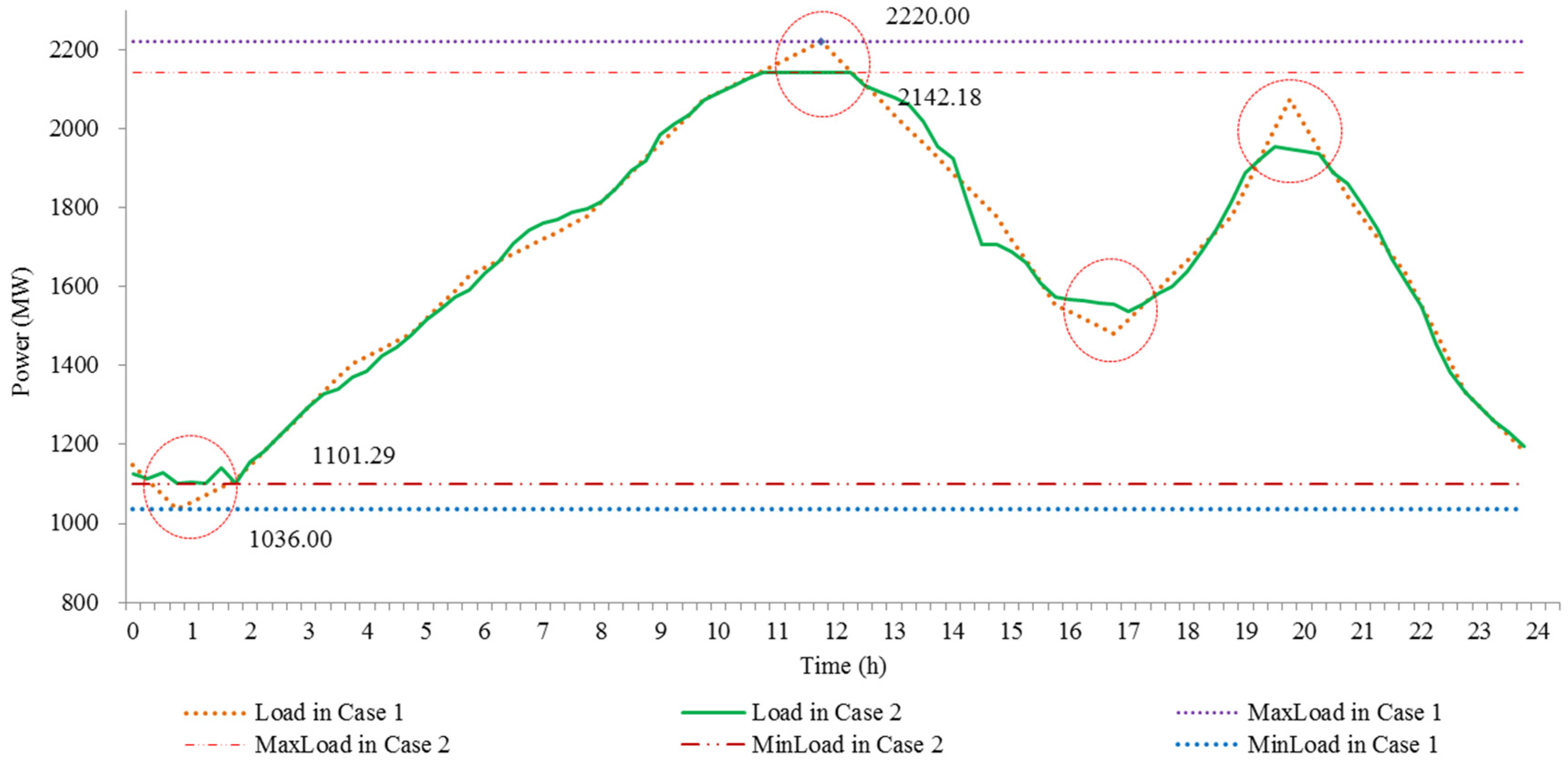
• Case 1: the power dispatch with wind farms and without SLBFLs. The spinning reserve confidence degree is 0.9.
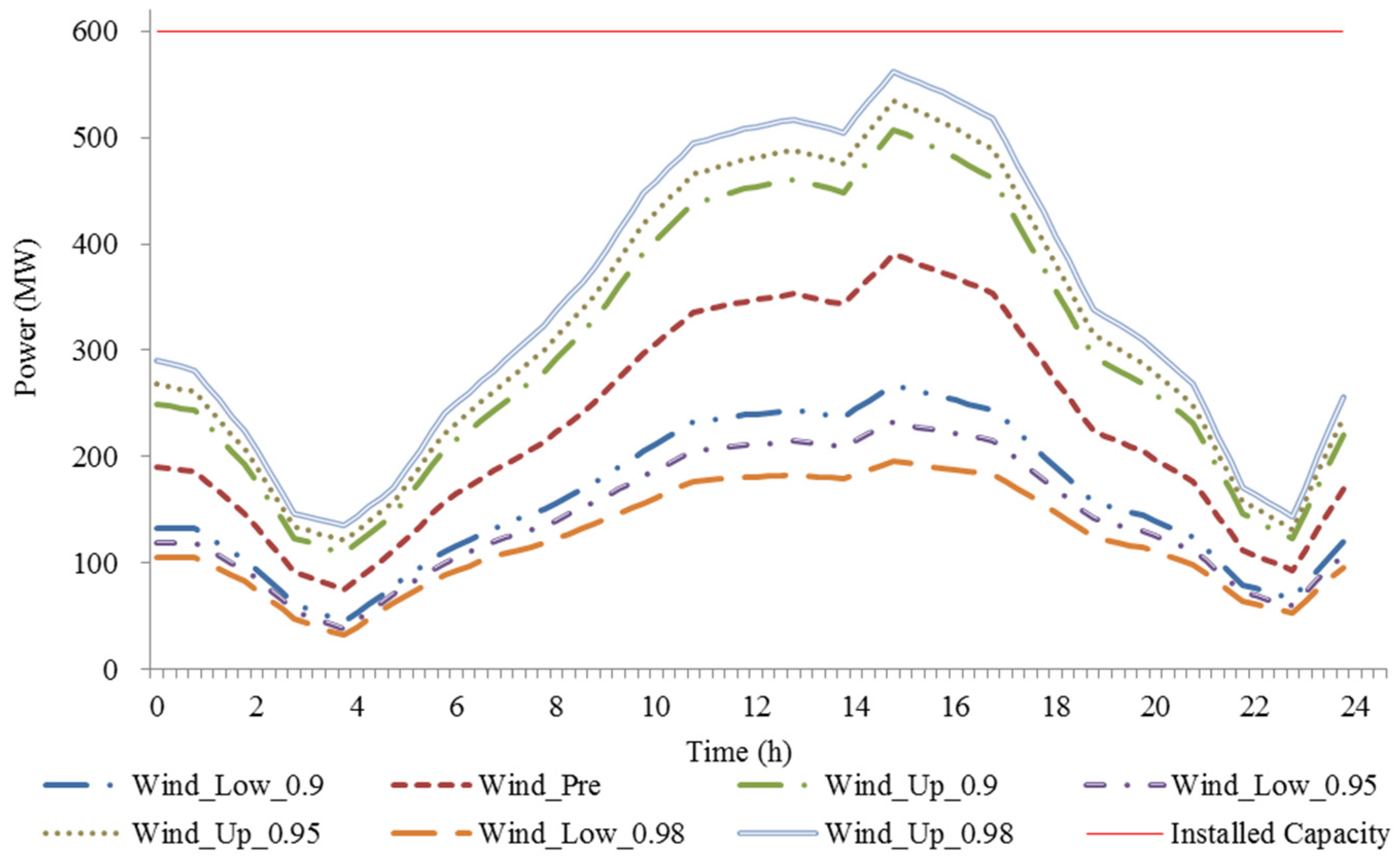
• Case 2: the power dispatch with wind farms and SLBFLs at wind power reserve confidence degree of 0.9, 0.95 and 0.98.
• Case 3: the power dispatch with SLBs on supply side and the spinning reserve confidence degree is 0.9.

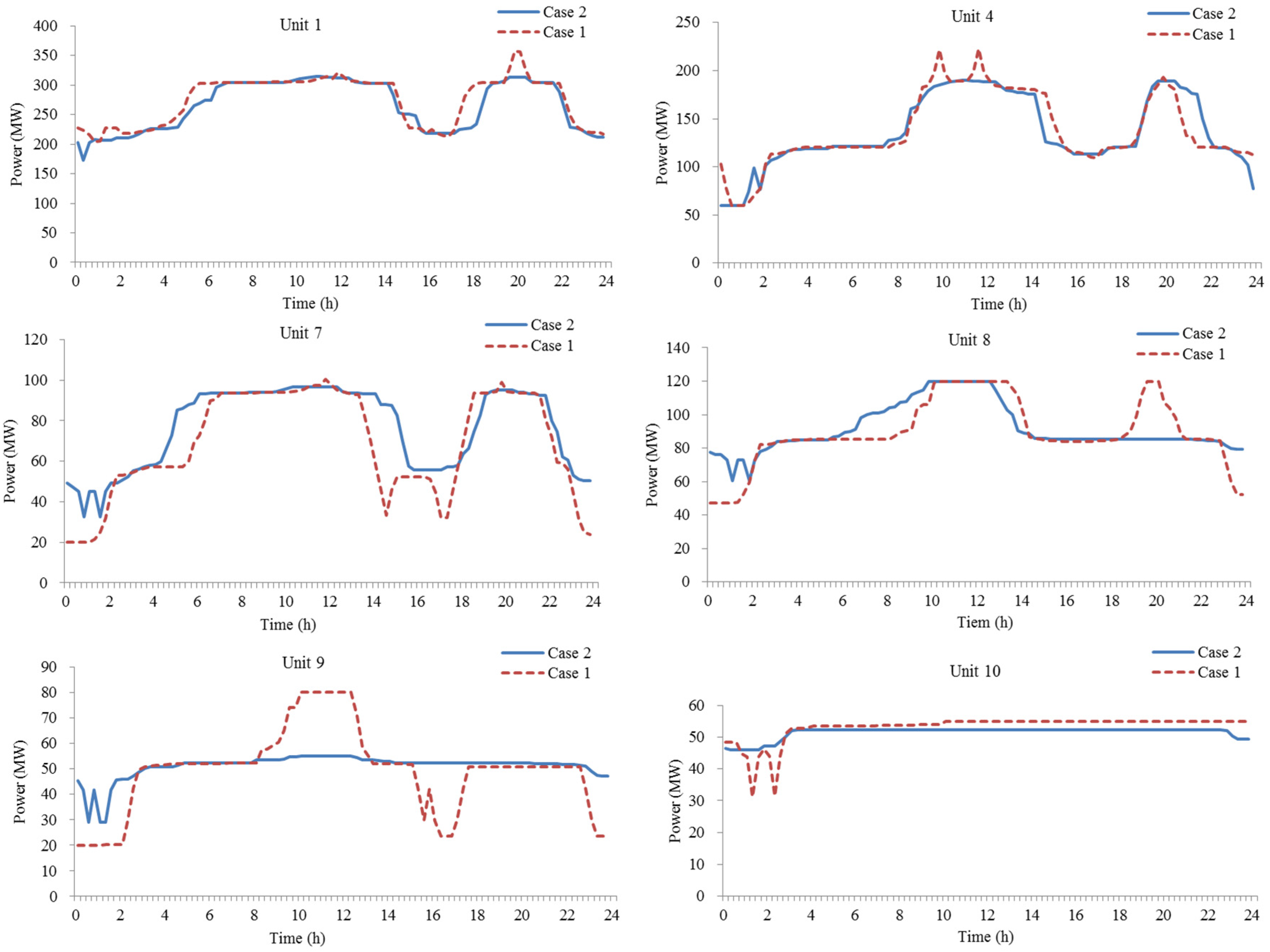
4.1. The Result Comparison of Case 1 and Case 2 with 0.9 Confidence Degree

The load curves are shown in Figure 9. The load peak-valley difference, system operating cost, thermal generating cost and thermal generator ramp cost in Cases 1 and 2 with 0.9 confidence degree are shown in Figure 10. Figure 11 presents the power generating curves in Cases 1 and 2 with 0.9 confidence degree, based on units 1, 4 and 7–10. The thermal generator ramp cost is reduced from $1.23 million to $0.97 million, the thermal power generating cost is decreased from $3.05 million to $2.83 million, and the system operating cost (including the thermal generation production cost, environmental emissions cost, spinning reserve cost and generators ramp cost) is reduced by 12% in Case 2 than in Case 1, as shown in Figure 10b.

The SLB test results are shown in Figure 10c. In Case 1, the OC is calculated as the maximum cost-saving from thermal generators with equal power outputs to SLBs. This is $13.26 million for Unit 2. The OC of SLBFLs in Case 2 is the maximum value of the alternative choice that SLBs are recycled as the metal material. This is $9.23 million from the recycling profit. The prices and the recycling rate of the metal materials are listed in

Table 3. Recycling rates and profit for battery materials [46,47,48].

Component	Component Percentage	Recycling Rate	Recycle Price ($/kg)
Aluminum	3.5%	42%	1.68
Cobalt	15%	89%	33.59
Lithium	1.8%	80%	62.5
Iron/steel	50%	52%	0.05

and the battery recycling coefficient is set at 70%. As a result, the total cost of the power system (operating cost and OC) with SLBFLs is 30% lower than that without SLBFLs, which is a staggering figure.

On the other hand, EVs can also participate in power dispatch (i.e., 1st-life batteries). Compared with SLBs, the power dispatch with EVs as flexible loads needs to take account of the time-of-use (TOU) electricity price and charging service fee in the economic analysis. These are shown in Figure 12 and the power outputs of SLBFLs are shown in Figure 13 for comparison. In Case 2 with 0.9 confidence degree, the total charging cost of using EVs as flexible loads is $0.28 million, which is much higher than using SLBFLs.

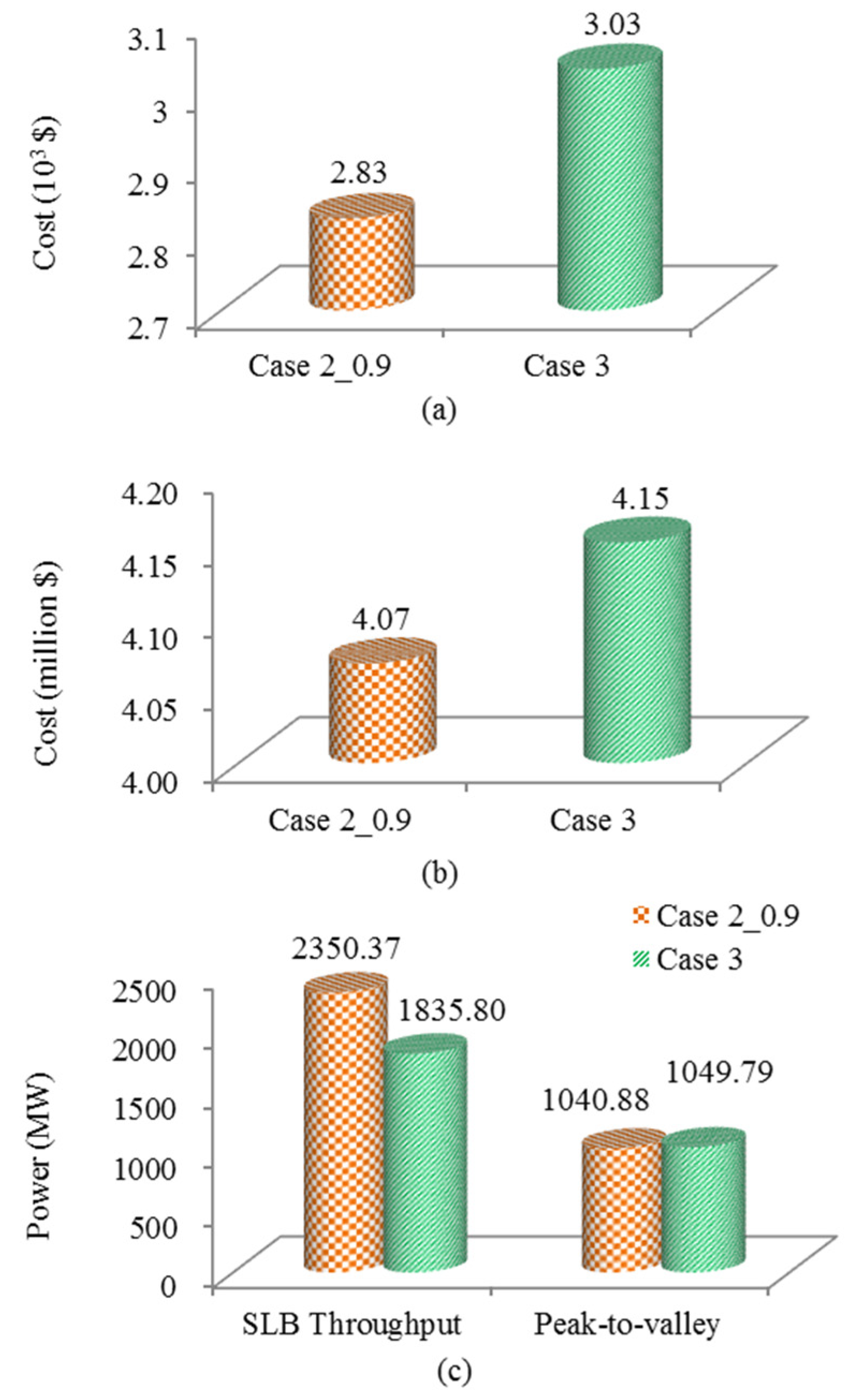
4.2. The Result Comparison of Case 2 and Case 3

The thermal power generating cost and system operating cost are shown in Figure 14a, the SLB throughput and load peak-to-valley are shown in Figure 14c. From these results, SLBs used on the load side as flexible loads are financially beneficial in power dispatch. The thermal power generating cost of Case 2 is 7% lower than that in Case 3, and the system operating cost in Case 2 is 2% lower than that in Case 3. The SLB throughput in Case 2 is 28% higher than that in Case 2 while the load peak-valley difference is 8.91 MW lower than in Case 3.

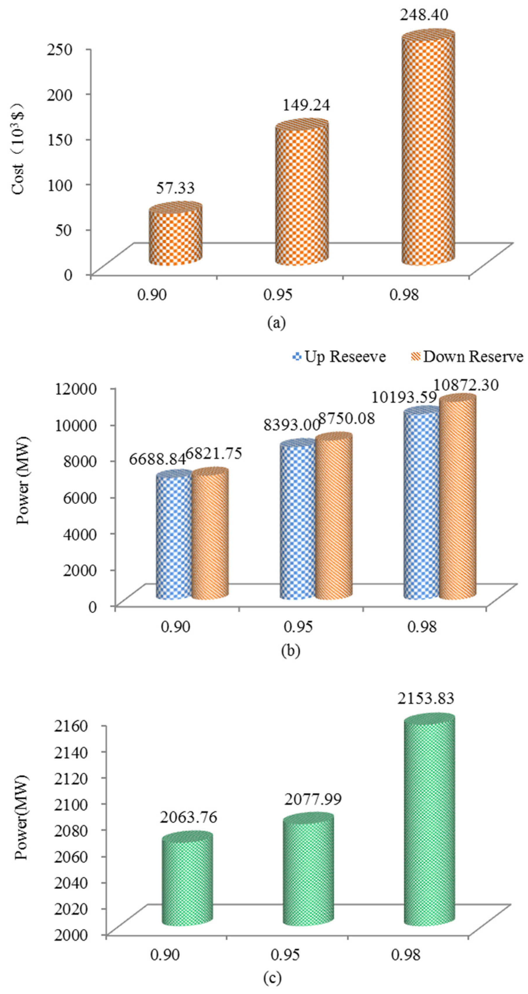
4.3. The Result Comparison of Case 2 with Different Confidence Degrees

Case 2 is the power dispatch with wind farms and SLBFLs while the wind power reserve confidence degree is set at 0.9, 0.95 and 0.98. It can be seen from Figure 15a,b, the system reserve cost, the up-reserve and down-reserve values at confidence degree 0.9 are the lowest, followed by those at 0.95 and 0.98 confidence degrees. The SLBFL throughput at different confidence degrees is shown in Figure 15c. It is clear that the SLBFL throughput increases with the wind power uncertainty.

5. Discussion

It becomes clear in Figure 10 that the penetration of wind power gives rise to fluctuations and disruption to thermal power plants, and there is little adjustment on the traditional loads to help balance this change. With the SLBFLs on the load side, the peak loads can be shaved to a lower level and the valley loads can be shifted to a higher level, which effectively reduces the peak-to-valley of the load curve. In this case, the maximum peak load is decreased from 2220 MW to 2142.18 MW and the minimum valley load is increased from 1036 MW to 1101.29 MW. Thus the peak-valley difference is improved from 1184 MW to 1114.2 MW, as shown in Figure 10a.

It can be seen from Figure 11 that the power generating curves are more smooth with SLBs and the fluctuations of thermal generator outputs in Case 2 is lower than that in Case 1. The flexible adjustment on the load side allows the generators to operate more stably. The SLBFLs can improve the adjustment capability of loads, which effectively aids thermal power plants in compensating the intermittence and fluctuation of the uncertainty. As a result, the thermal generator ramp cost, the thermal power generating cost and the system operating cost are all reduced, shown in Case 2.

From Figure 12 and Figure 13, the power dispatch with EVs as flexible loads will need additional electricity tariffs and charging fee to be economically viable. With the same charging capacity, the cost of utilizing SLBFLs is much cheaper. In addition, the SLBFLs can provide a large amount of electrical power to the power grid whilst EVs are difficult to match. Therefore, SLBs are more suitable to be connected to the power system for system stability.

Similarly, Figure 14 also revealed that it is better to connect SLBs on the load side than the supply side, from the economic perspective. SLBFLs can reduce the peal-valley difference of load, which reduces the fluctuation of the supply. Thermal generators can then run more smoothly so as to lower their ramp costs and operation costs. In this work, the power dispatch decisions in Case (3) are based on the optimization process, whilst the ramp cost of individual generator can be increased or decreased. This again confirms that the SLBs are better to be placed on the load side of the system.

Figure 15 shows the spinning reserve cost, up-reserve and down-reserve of wind power and the total output of SLBFLs in Case 2. A higher confidence figure means more uncertainty of wind power is in the consideration of power dispatch, leading to a higher spinning reserve needed in the power dispatch (i.e., higher reserve cost). In essence, a high uncertainty of wind power in the power system makes it difficult to achieve the power balance. Moreover, the SLBFL throughput increases with the wind power uncertainty as Figure 15c suggests.

6. Conclusions

This paper has presented a stochastic day-ahead economic power dispatch model with wind farms and SLBFLs at MW levels. The SLB characteristics are studied for economic dispatch purposes. Based on the actual data from NASA batteries, the impact of battery temperatures and charging/discharging currents on the SLB performance is evaluated in order to participate in the power dispatch. A new optimization strategy is proposed to achieve the power balance of the power system and also to minimize the operating cost and environmental emissions cost. In the power dispatch model, the SLBs perform as flexible loads to decrease the fluctuation of thermal power plants and the load peak-valley difference. A study on a ten-unit power system is carried out in three cases and a prime-dual interior point method is used to optimize the system costs.

The test results show that SLBFLs can reduce the load fluctuation so as to realize the peak-load shifting. Compared with SLBs to be disposed of, the opportunity cost of SLBs used as flexible loads is lower and more environmentally-friendly. The system operating cost with wind farms and SLBFLs is reduced by 12%. The SLBFL throughput, reserve power and operating cost all have similar trends with the confidence degrees. Compared with utilizing EVs as flexible loads, SLBFLs can reduce $0.28 million of the system operating cost. Moreover, the economy of power dispatch with the SLBs on the load side is better than that on the supply side, as well as the reduced peak-valley difference. This work will have significant economic implications and environmental benefits for both automotive industry and power industry in utilizing waster batteries as flexible loads for power support.

References

1. Kim, C.; Muljadi, E.; Chung, C.C. Coordinated Control of Wind Turbine and Energy Storage System for Reducing Wind Power Fluctuation. Energies 2018, 11, 52. [Google Scholar] [CrossRef]
2. Liu, J.T.; Feng, S.H.; Wang, K.; Guo, X.R.; Xu, L.Z. Method to determine spinning reserve requirement for a grid with large-scale wind power penetration. J. Eng. 2017, 2017, 1686–1691. [Google Scholar] [CrossRef]
3. Qin, B.; Liu, D.; Cao, M.; Zou, J. Formal modeling and verification of flexible load control for power grid CPS based on differential dynamic logic. In Proceedings of the 2017 IEEE Conference on Energy Internet and Energy System Integration (EI2), Beijing, China, 26–28 November 2017; pp. 1–6. [Google Scholar]
4. González, F.D.; Sumper, A.; Bellmunt, O.G.; Robles, R.V. A review of energy storage technologies for wind power applications. Renew. Sustain. Energy Rev. 2012, 16, 2154–2171. [Google Scholar] [CrossRef]
5. Wang, K.; Yao, J.; Yao, L.; Yang, S.; Yong, T. Survey of research on flexible loads scheduling technologies. Autom. Electr. Power Syst. 2014, 38, 127–135. [Google Scholar]
6. Moghaddam, I.N.; Chowdhury, B.H.; Mohajeryami, S. Predictive Operation and Optimal Sizing of Battery Energy Storage With High Wind Energy Penetration. IEEE Trans. Ind. Electron. 2018, 65, 6686–6695. [Google Scholar] [CrossRef]
7. Dui, X.; Zhu, G.; Yao, L. Two-Stage Optimization of Battery Energy Storage Capacity to Decrease Wind Power Curtailment in Grid-Connected Wind Farms. IEEE Trans. Power Syst. 2018, 33, 3296–3305. [Google Scholar] [CrossRef]
8. Hu, J.; Sarker, M.R.; Wang, J.; Wen, F.; Liu, W. Provision of flexible ramping product by battery energy storage in day-ahead energy and reserve markets. IET Gener. Transm. Distrib. 2018, 12, 2256–2264. [Google Scholar] [CrossRef]
9. Cai, H.; Chen, Q.; Guan, Z.; Huang, J. Day-ahead optimal charging/discharging scheduling for electric vehicles in microgrids. Prot. Control Mod. Power Syst. 2018, 73, 9. [Google Scholar] [CrossRef]
10. Li, J.L.; Xiu, X.Q.; Liu, D.T.; Hui, D. Research on Second Use of Retired Electric Vehicle Battery Energy Storage System Considering Policy Incentive. High Volt. Eng. 2015, 42, 2562–2568. [Google Scholar]
11. Ma, J.; Ma, Q.B. Development status and tendency of electric vehicles in China. Mech. Equip. 2017, 48, 44. [Google Scholar]
12. Xia, M.; Lai, Q.; Zhong, Y.; Li, C.; Chiang, H.D. Aggregator-Based Interactive Charging Management System for Electric Vehicle Charging. Energies 2016, 9, 159. [Google Scholar] [CrossRef]
13. Sun, H.; Shen, Z.H.; Zhou, W.; Hu, S.B.; Ma, Q.; Chen, X.D.; Li, C.P.; Yang, W.Q. Congestion Dispatch Research of Active Distribution Network With Electric Vehicle Group Response. Proc. CSEE 2017, 19, 5549–5559. [Google Scholar]
14. Godina, R.; Paterakis, N.G.; Erdinç, O.; Rodrigues, E.M.G.; Catalão, J.P.S. Electric vehicles home charging impact on a distribution transformer in a Portuguese Island. In Proceedings of the International Symposium on Smart Electric Distribution Systems and Technologies, Vienna, Austria, 8–11 September 2015; pp. 74–79. [Google Scholar]
15. Viswanathan, V.V.; Kintner-Meyer, M. Second use of transportation batteries: Maximizing the value of batteries for transportation and grid services. IEEE Trans. Veh. Technol. 2011, 60, 2963–2970. [Google Scholar] [CrossRef]
16. Development Status and Tendency of EV Battery Recycling and Utilization. Available online: http://shupeidian.bjx.com.cn/news/20180112/873651.shtml (accessed on 12 January 2018).
17. Joseph, A.; Shahidehpour, M. Battery storage systems in electric power systems. In Proceedings of the Power Engineering Society General Meeting, Montreal, QC, Canada, 18–22 June 2006; p. 8. [Google Scholar]
18. Viswanathan, V.V.; Kintner-Meyer, M. Energy efficiency evaluation of a stationary lithium-ion battery container storage system via electro-thermal modeling and detailed component analysis. Appl. Energy 2018, 210, 211–229. [Google Scholar]
19. Ciobotaru, C.K.; Saez-De-Ibarra, A.; Laserna, E.M.; Stroe, D.I.; Swierczynski, M.; Rodriguez, P. Second Life Battery Energy Storage System for Enhancing Renewable Energy Grid Integration. In Proceedings of the Energy Conversion Congress & Exposition (ECCE), Montreal, QC, Canada, 20–24 September 2015; pp. 78–84. [Google Scholar]
20. Kazakos, S.S.; Daniel, S.; Buckley, S. Distributed energy storage using second-life electric vehicle batteries. In Proceedings of the Power in Unity: A Whole System Approach, London, UK, 16–17 October 2014; pp. 1–6. [Google Scholar]
21. Gladwin, D.T.; Gould, C.R.; Stone, D.A.; Foster, M.P. Viability of ‘second-life’ use of electric and hybrid-electric vehicle battery packs. In Proceedings of the Industrial Electronics Society, IECON 2013—39th Annual Conference, Vienna, Austria, 10–13 November 2014; pp. 1922–1927. [Google Scholar]
22. Martinez-Laserna, E.; Sarasketa-Zabala, E.; Villarreal, I.; Stroe, D.I.; Swierczynski, M.; Warnecke, A.; Jean-Marc, T.; Goutam, S.; Omar, N.; Rodriguez, P. Technical viability of battery second life: A study from the ageing perspective. IEEE Trans. Ind. Appl. 2018, 54, 2703–2713. [Google Scholar] [CrossRef]
23. Debnath, U.K.; Ahmad, I.; Habibi, D. Gridable vehicles and second life batteries for generation side asset management in the Smart Grid. Electr. Power Energy Syst. 2016, 82, 114–123. [Google Scholar] [CrossRef]
24. Hernández, J.C.; Sanchez-Sutil, F.; Vidal, P.G.; Rus-Casas, C. Primary frequency control and dynamic grid support for vehicle-to-grid in transmission systems. Int. J. Electr. Power Energy Syst. 2018, 100, 152–166. [Google Scholar] [CrossRef]
25. Cheng, Y.; Zhang, C. Configuration and operation combined optimization for ev battery swapping station considering PV consumption bundling. Prot. Control Mod. Power Syst. 2017, 2, 26. [Google Scholar] [CrossRef]
26. Gerssen-Gondelach, S.J.; Faaij, A.P.C. Performance of batteries for electric vehicles on short and longer term. J. Power Sources 2012, 212, 111–129. [Google Scholar] [CrossRef] [Green Version]
27. Yang, R.; Xiong, R.; He, H.; Mu, H.; Wang, C. A novel method on estimating the degradation and state of charge of lithium-ion batteries used for electrical vehicles. Appl. Energy 2017, 207, 336–345. [Google Scholar] [CrossRef]
28. Abdel-Monem, M.; Hegazy, O.; Omar, N.; Trad, K.; Bossche, P.V.D.; Mierlo, J.V. Lithium-ion batteries: Comprehensive technical analysis of second-life batteries for smart grid applications. In Proceedings of the 2017 19th European Conference on Power Electronics and Applications (EPE’17 ECCE Europe), Warsaw, Poland, 11–14 September 2017; pp. 1–16. [Google Scholar]
29. Baumann, M.; Rohr, S.; Lienkamp, M. Cloud-connected battery management for decision making on second-life of electric vehicle batteries. In Proceedings of the 2018 Thirteenth International Conference on Ecological Vehicles and Renewable Energies (EVER), Monte-Carlo, Monaco, 10–12 April 2018; pp. 1–6. [Google Scholar]
30. Graber, G.; Galdi, V.; Calderaro, V.; Mancarella, P. A stochastic approach to size EV charging stations with support of second life battery storage systems. In Proceedings of the 2017 IEEE Manchester PowerTech, Manchester, UK, 18–22 June 2017; pp. 1–6. [Google Scholar]
31. Li, R. Research on Evaluation and Estimation Methods for State of Health of Power Lithium Iron Battery. Ph.D. Thesis, Harbin University of Science and Technology, Harbin, China, June 2016. [Google Scholar]
32. Zhang, H. Energy Storage Optimization Planning Considering Second-Use Batteries. Master’s Thesis, North China Electric Power University, Beijing, China, March 2017. [Google Scholar]
33. Tong, S.; Fung, T.; Park, J.W. Reusing Electric Vehicle Battery for Demand Side Management integrating Dynamic Pricing. In Proceedings of the IEEE International Conference on Smart Grid Communications, Miami, FL, USA, 2–5 November 2015; pp. 325–330. [Google Scholar]
34. Castano, S.; Jimenez, D.S.; Sanz, J. BMS influence on Li-ion packs characterization and modeling. In Proceedings of the 2016 IEEE 16th International Conference on Environment and Electrical Engineering (EEEIC), Florence, Italy, 7–10 June 2016; pp. 1–6. [Google Scholar]
35. Saha, B.; Goebel, K.; Battery Data Set. NASA Ames Prognostics Data Repository. 2007. Available online: http://ti.arc.nasa.gov/project/prognostic-data-repository (accessed on 16 November 2017).
36. Chen, L.; Ji, B.; Cao, W.P.; Pan, H.H.; Tian, B.B.; Lin, W.L. Grey system theory-based capacity estimation method for Li-ion batteries. In Proceedings of the 7th IET International Conference on Power Electronics, Machines and Drives (PEMD 2014), Manchester, UK, 8–10 April 2014; pp. 1–5. [Google Scholar]
37. Li, Y.Z. Discussion of “adaptive robust optimization for the security constrained unit commitment problem”. IEEE Trans. Power Syst. 2014, 29, 996. [Google Scholar] [CrossRef]
38. Zhou, W.; Peng, Y.; Sun, H.; Wei, Q.H. Dynamic economic dispatch in wind power integrated system. Proc. CSEE 2009, 29, 13–18. [Google Scholar]
39. Rebours, Y.; Kirschen, D.; Trotignon, M. Fundamental design issues in markets for ancillary services. Electr. J. 2007, 20, 26–34. [Google Scholar] [CrossRef]
40. Liu, J.C.; Li, D.F. Corrections to “TOPSIS-Based Nonlinear-Programming Methodology for Multi-attribute Decision Making With Interval-Valued Intuitionistic Fuzzy Sets. IEEE Trans. Fuzzy Syst. 2018, 26, 391. [Google Scholar] [CrossRef]
41. Liu, X. Impact of beta-distributed wind power on economic load dispatch. Electr. Power Compon. Syst. 2011, 39, 768–779. [Google Scholar] [CrossRef]
42. Zhang, H.F.; Gao, F.; Wu, J.; Liu, K. A Dynamic Economic Dispatching Model for Power Grid Containing Wind Power Generation System. Power Syst. Technol. 2013, 37, 1298–1303. [Google Scholar]
43. Shen, Z.; Xie, S.Q.; Pan, C.Y. Probability and Statistics; High Education Press: Beijing, China, June 2008; pp. 139–143, 161–163. [Google Scholar]
44. Attaviriyanupap, P.; Kita, H.; Tanaka, E.; Hasegawa, J. A hybrid EP and SQP for dynamic economic dispatch with nonsmooth fuel cost function. IEEE Trans. Power Syst. 2002, 17, 411–416. [Google Scholar] [CrossRef]
45. Zhang, X.H.; Zhao, J.Q.; Chen, X.Y. Multi-objective Unit Commitment Fuzzy Modeling and Optimization for Energy-saving and Emission Reduction. Proc. CSEE 2010, 30, 71–76. [Google Scholar]
46. Wang, X.; Gaustad, G.; Babbitt, C.W.; Richa, K. Economies of scale for future lithium-ion battery recycling infrastructure. Resour. Conserv. Recycl. 2014, 83, 53–62. [Google Scholar] [CrossRef]
47. Jin, Q.H. Recycling Modes of Power Batteries of Electric Vehicles Based on Product Life Cycle. Master’s Thesis, Huazhong University of Science and Technology, Wuhan, China, April 2016. [Google Scholar]
48. USGS. Mineral Commodity Summaries 2012. U.S. Geological Survey, 2012. Available online: https://minerals.usgs.gov/minerals/pubs/mcs/2012/mcs2012.pdf (accessed on 20 April 2018).
Figure 1. Battery discharging characteristics at different temperatures and currents.
Energies 11 01657 g001
Figure 2. Battery actual characteristic curve fitting. (a) is Battery B0039 actual power-SOC curve fitting; (b) is Battery B0039 actual temperature-SOC curve fitting; (c) is Battery B0006 actual power-SOC curve fitting and (d) is Battery B0006 actual temperature-SOC curve fitting.
Energies 11 01657 g002
Figure 3. Battery cells are dismantled from electric vehicle (EV) and regrouped to a second life batteries (SLB) pack.
Energies 11 01657 g003
Figure 4. Schematic diagram of the proposed power grid.
Energies 11 01657 g004
Figure 5. The Beta distribution curve.
Energies 11 01657 g005
Figure 6. Flow charts. (a) is the flow chart of economic dispatch optimization and (b) is the flow chart of Interior point method.
Energies 11 01657 g006
Figure 7. Daily load demand curve.
Energies 11 01657 g007
Figure 8. Predicted wind power and wind power bounds at different confidence degrees.
Energies 11 01657 g008
Figure 9. Load curves of Case 1 and Case 2 with 0.9 confidence degree.
Energies 11 01657 g009
Figure 10. Result comparisons of Case 1 and Case 2 with 0.9 confidence degree. (a) is load peak-valley differences; (b) is system operating cost, thermal power generating cost and thermal generator ramp cost and (c) is the OC of SLBs to be disposed of and used as flexible loads.
Energies 11 01657 g010
Figure 11. Active power generating curves of Unit 1, Unit 4 and Units 7–10 in Case 1 and Case 2 with 0.9 confidence degree.
Energies 11 01657 g011
Figure 12. Time-of-use (TOU) electricity price and charging fee.
Energies 11 01657 g012
Figure 13. SLB power outputs.
Energies 11 01657 g013
Figure 14. Results comparison of Case 3 and Case 2 with 0.9 confidence degree. (a) is the thermal generating cost comparison; (b) is the system operation cost comparison and (c) is the SLB throughput and peak-to-valley comparison.
Energies 11 01657 g014
Figure 15. The results of Case 2 at different confidence degrees; (a) is the spinning reserve cost; (b) is the up-reserve and down-reserve of wind power and (c) is the total output of SLBFLs.
Energies 11 01657 g015