A Novel Hybrid DC Traction Power Supply System Integrating PV and Reversible Converters

Abstract

A novel hybrid traction power supply system (HTPSS) integrating PV and reversible converter (RC) is proposed. PV is introduced to reduce the energy cost and increase the reliability of power systems. A reversible converter can achieve multiple objectives including regenerative braking energy recovery, PV energy inverting, DC voltage regulation and power factor improvement. In this paper, the topology and operating modes of the HTPSS are first introduced. Three-level boost converter (TLBC) is employed in the PV system. A double closed-loop control scheme considering both maximum power point tracking (MPPT) and midpoint potential balancing (MPB) is recommended. The reversible converter adopts a multi-modular topology and the independent control for active power and reactive power has been achieved by a current decoupling control. According to the working characteristic of each device, a coordinated control strategy is designed, and four basic principles are given. A system simulation model containing a hybrid traction substation and a train was built, and comprehensive simulations under multi-scenario were carried out. The results show that the reversible converter can accomplish PV energy inversion, DC voltage regulation, regenerative braking energy recovery and power factor improvement, by which a high utilization rate and energy-saving effect can be obtained.

1. Introduction

In an urban Traction Power Supply System (TPSS), diode rectifiers are usually used as the power supply devices. The merits of this conventional power supply mode are that it is simple, robust and low-cost. However, its drawbacks are also obvious. When there is not enough train in traction state on the line, the regenerative braking energy cannot be completely reused within the DC network [1]. Some of the regenerative braking energy has to be dissipated in the on-board braking resistors, causing huge energy waste and noticeable tunnel temperature rise [2]. In addition, capacitance distributed in a large amount of medium voltage cables leads to very low power factor during light-load period, which has to be solved by special reactive power compensating equipment such as SVG [3,4,5].

A few decades ago, inverters were introduced into DC traction power supply system to recover the regenerative braking energy [6,7,8]. Compared to energy storage equipment [9,10,11], inverters show considerable advantages in cost, reliability and installing space, so have been paid more and more attention [12,13,14]. However, inverters installed in the substations do not work all the time. When a train runs between two substations, the braking time is only 10–15 s under normal circumstances. The relatively low utilization rate, in addition to the single function (just inverting), result in a long investment payback period. It is becoming the main obstacle for the massive application of inverters.

Urban rail transit is becoming a big energy consumer and has significant impacts on energy consumption at a regional scale [15]. It turns out to be more and more urgent to reduce system energy consumption through all possible means. As a clean energy, photovoltaic has had rapid development all over the world recently, and the installed capacity has been increasing year by year [16,17]. Large-scale PV plants are mainly located in the desert regions due to the high solar irradiance and vast area, but the output power is usually constrained by the transmission capacity of the grid [18]. Future development will focus on the distributed PV system, which is located as close to the user as possible [19]. Railway companies have much potential to introduce PV system around railway premises, such as the roof of platforms, substations, vehicle depots, sound walls and other buildings or openings along the line [20]. It is reported that the PV system installed on platform roof of Tokyo station generates 340 MWh electric energy annually [20]. The possibility of introducing PV technologies into traction power supply system is discussed in [21], but solar energy is just used for air conditioning and lighting. In [22], a grid-connected PV system is introduced in TPSS. However, it is not an optimal scheme for the transmission and distribution of solar energy. In [23], PV is introduced to provide energy for the tramway, but the expensive energy storage device has to be installed at the same time. In [24], the feasibility and application modes of PV in urban rail transit have been studied, and the results show that the DC network-connected mode can maximize the benefits of PV generation system. However, the coordinated control between PV system and train is not considered in detail.

In this paper, a novel hybrid DC traction power supply system integrating both PV and reversible converter is proposed. The combination of PV system and reversible converter can significantly reduce electricity bill, improve reliability and power quality of the power system.

The DC/DC converter in a PV system normally plays the role of voltage boost and MPPT control [25,26,27]. A three-level boost converter (TLBC) is employed in this paper. Compared to conventional two-level boost converter, the TLBC is more widely employed in high-voltage high-power applications to reduce the device voltage stress, to increase the power ratings, and to decrease the output filter size [28,29,30,31,32,33,34]. However, TLBC has to face the problem of midpoint potential shift in practical applications. As a result, the voltage of the two output capacitors will be unbalanced, and the switching devices will confront unequal voltage and current stress [28,29,31]. To achieve the midpoint potential balance of the two capacitors, different control methods have been studied in the literature. According to pulse generation modes, the control methods can be divided into two categories: independent duty-ratio control [35,36,37] and pulse phase-shift control [38,39]. The independent duty-ratio control strategy can effectively reduce the deviation voltage. However, the output voltage control variable and the deviation voltage control variable have a complex coupling relationship. The pulse phase-shift control strategy, by contrast, can achieve relatively independent control of deviation voltage without affecting the output characteristics of the TLBC. For the pulse phase-shift control strategy, few studies focus on the analysis of regulation ability for the deviation voltage.

The reversible converter has a similar main circuit as conventional inverter but can realize the bidirectional energy flow and flexible power factor regulation [40]. For small and medium power application, two-level voltage source topology is commonly used. For high power application, the multi-modular topology should be adopted to enlarge capacity, reduce harmonics, and make the maintenance fast and easy [41]. The current decoupling control scheme based on dq rotating frame is widely employed by reversible converters to achieve an independent regulation for active current and reactive current. In most cases, the active current reference comes from a DC voltage regulator to keep the voltage constant, and the reactive current reference is set to zero [42]. However, for the proposed application, some specific change should be made.

Many studies have focused on the PV system or reversible converter, but none of them focuses on the combination of them. It should be a good idea to introduce both the PV system and reversible converter into the urban DC traction power supply system, making up HTPSS. It can be regarded as a DC microgrid [43], which includes diode rectifiers, reversible converters, TLBCs, solar panels and trains. The reversible converter will be the crucial part of the HTPSS. Besides the PV energy inverting, the reversible converter is also put in charge of DC voltage regulation, train’s braking energy recovering, as well as power factor improvement. The control method will change from the conventional single-objective control to the new multi-objective control. The coordinated control with other equipment in the system will be of great importance. Thus far, few studies have focused on the similar coordinated control strategy.

This paper mainly focuses on the main circuit and control of the HTPSS. The structure is organized as follows. In Section 2, the topology and operating modes of the proposed HTPSS are introduced. In Section 3, the main circuit of TLBC is introduced and a control method for midpoint potential balancing based on pulse phase-shift is proposed, which was tested by prototype experiment. Section 4 introduces the main circuit and current control of the reversible converter. In Section 5, the working characteristics of main components are studied, and a system coordinated control strategy is designed. Finally, the effectiveness of the proposed HTPSS and corresponding control strategy are verified by Matlab/Simulink.

2. Topology and Operating Modes of the HTPSS

2.1. Topology of the HTPSS

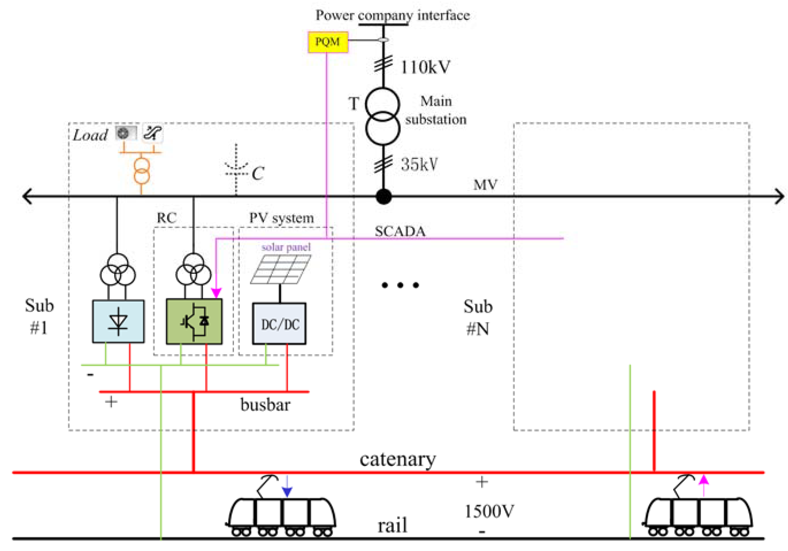
The topology of the HTPSS is shown in Figure 1. It can be seen that a PV system and a reversible converter are added to each substation. The AC side of the reversible converter is connected to medium voltage (MV) grid, and its DC link is connected to the DC busbar of the substation. The PV system is connected to the DC busbar through a DC/DC converter. C denotes the equivalent capacitance of the AC cable. T denotes the step-down transformer in the main substation. A power quality meter (PQM) is installed at the interface with the power company. The information of PQM can be sent to reversible converter of each substation by network, such as Supervisory Control And Data Acquisition (SCADA).

In this paper, the DC/DC converter in PV system employs three-level boost converter (TLBC), which has obvious advantages, such as reducing device voltage stress, increasing the power ratings, and cutting output filter size. Due to the special relationship of the output voltage and current of the solar panels, the MPPT should be carried out by TLBC to convert as much solar energy as possible to the DC busbar. The energy can be used by train directly, thus it is highly efficient since there is no power loss on the inverter. If the solar energy is larger than the power required by train, it will be fed back to medium voltage grid through a reversible converter. The capacity of the PV system is determined by the average power demand of the traction substation and the available installation space for solar panels.

A high power reversible converter can be used to accomplish multiple functions. The reversible converter will be controlled to work at rectifying state or inverting state according to the state of the train and PV system, aiming to achieve a better DC voltage stability and energy-saving effect. In addition, the reversible converter can generate a certain amount of reactive power to improve the power factor of the medium voltage grid and replace the special reactive power compensation equipment such as SVG.

The diode rectifier, which is a conventional 12-pulse rectifier based on the multi-winding phase-shift transformer, can guarantee the reliability of the power supply system in the case of the failure of PV system and reversible converter.

2.2. Operating Modes of the HTPSS

Taking a single substation as an example, the possible operating modes are shown in Figure 2.

Table 1. Definition of the abbreviation.

Abbreviation	Definition	Abbreviation	Definition
DR	12-pulse rectifier	$P_{\mathrm{dr}}$	power of DR
RC	reversible converter	$P_{\mathrm{rc}}$	power of RC
PV	TLBC and PV array	$P_{\mathrm{pv}}$	power of PV
TR	train	$P_{\mathrm{tr}}$	power of TR
$P_{\mathrm{rc}\_\max }$	maximum power of RC	$V_{\mathrm{sub}}$	DC voltage of substation
$P_{\mathrm{pv}\_\max }$	maximum power of PV	$V_{\mathrm{dio}}$	no-load voltage of DR

lists the abbreviations used in the analysis below.

Typical operating modes are explained in

Table 2. Explanation of the typical operating modes.

Mode	Explanation
(a)	No power is required by the train, that is $P_{\mathrm{tr}}=0$. The power produced by PV is completely fed back to MV grid. DR is in blocked state.
(b)	The power required by the train is less than the power produced by PV, that is $P_{\mathrm{tr}}<P_{\mathrm{pv}}$. Part of PV power is fed back to MV grid. DR is blocked. DR is in blocked state.
(c)	The power required by the train is equal to the power produced by PV, that is $P_{\mathrm{tr}}=P_{\mathrm{pv}}$. DR is in blocked state.
(d)	The power required by the train is more than the power produced by PV, that is $P_{\mathrm{tr}}>P_{\mathrm{pv}}$. RC is activated to keep the DC voltage constant.
(e)	The power required by the train is more than the total power provided by PV and RC, that is $P_{\mathrm{tr}}>P_{\mathrm{pv}}+P_{\mathrm{rc}}$. Then, $V_{\mathrm{sub}}<V_{\mathrm{dio}}$, and the DR starts to work.
(f)	The train is in braking state. The total power generated by TR and produced by PV is equal to the power inverted by RC, that is $P_{\mathrm{tr}}+P_{\mathrm{pv}}=P_{\mathrm{rc}}$. Then, $V_{\mathrm{sub}}>V_{\mathrm{ido}}$, the DR returns to blocked state again.
(g)	The train is in braking state. The power generated by TR is equal to the maximum power of RC, that is $P_{\mathrm{tr}}=P_{\mathrm{rc}\_\max }$. The power produced by PV is reduced to zero automatically to avoid overvoltage.
(h)	When the power factor becomes low in the night or long headway time, the RC can generate compensating reactive power like a SVG.
(i)	The DR can continue to supply the TR in case of fault of RC and PV, but the system energy consumption will increase.

.

3. Three-Level Boost Converter

3.1. Main Circuit

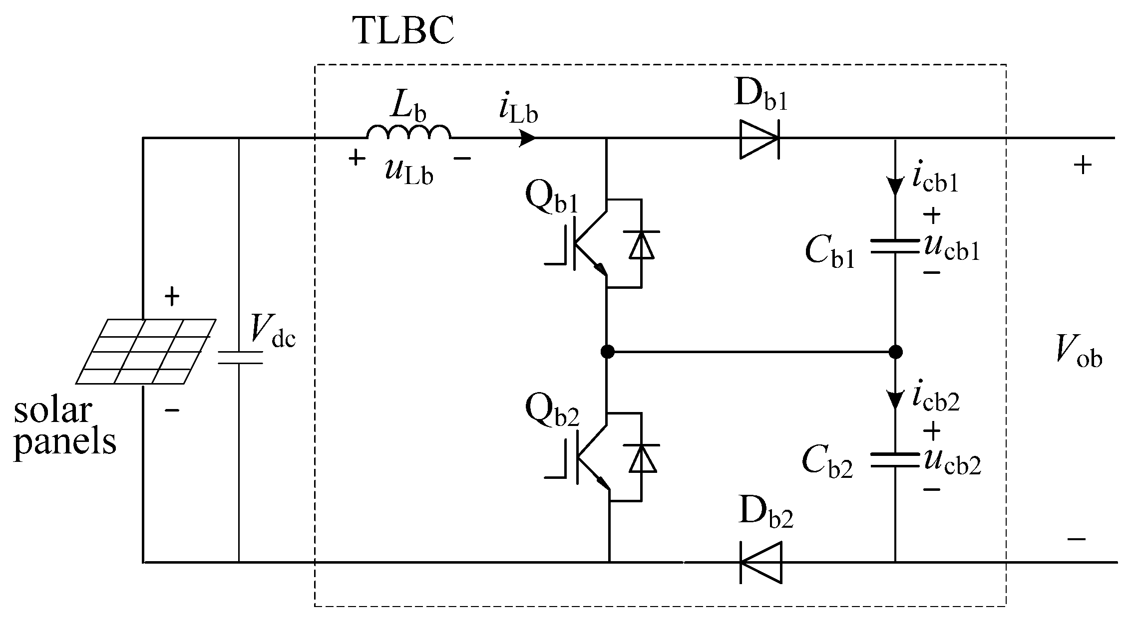
The main circuit of the TLBC is shown in Figure 3. L_b is the boost inductor, C_b1 and C_b2 are the output filtering capacitors, V_dc denotes the output voltage of the solar panels, u_cb1 and u_cb2 denote the voltage of two capacitors, and V_ob = u_cb1 + u_cb2 denotes the total output voltage of the TLBC.

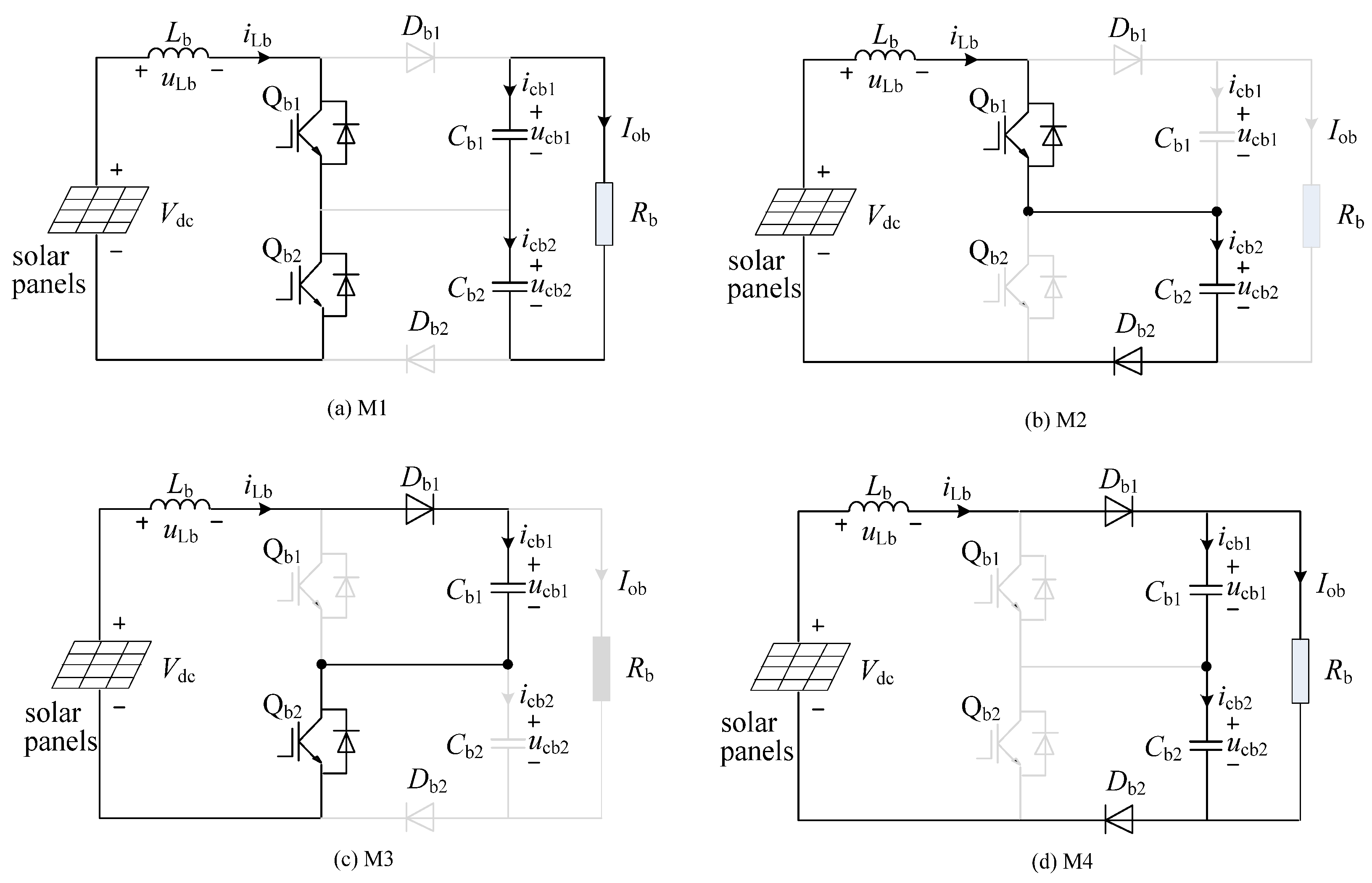
Due to the existence of L_b, D_b1 and D_b2, the main switch Q_b1 and Q_b2 can turn on at the same time without short-circuit fault. Therefore, there are four switching modes according to the state of two IGBTs and two diodes, as shown in Figure 4. A system mathematical model of four modes (M1–M4) can be established to describe the dynamic characteristics of the inductance current and the capacitance voltage using the Kirchhoff’s law [44].

3.2. Control Scheme

A double closed-loop control scheme is recommended in Figure 5, in which a MPPT control loop and a deviation voltage loop are included. i_pv denotes the output current of the solar panels. D_on-b denotes the output of MPPT control loop. ∆u_cb = u_cb1 − u_cb2 denotes the deviation voltage of the two capacitors. ∆u_cb-ref denotes the reference of deviation voltage loop (default value is zero). ∆u_ctrl denotes the output of deviation voltage loop. PWM denotes pulse generating unit.

Several kinds of MPPT methods are studied and compared in literature, but the Perturbation and observation (P & O) method is the most popular one [25,26], which will be adopted in this paper.

3.3. Midpoint Potential Balancing

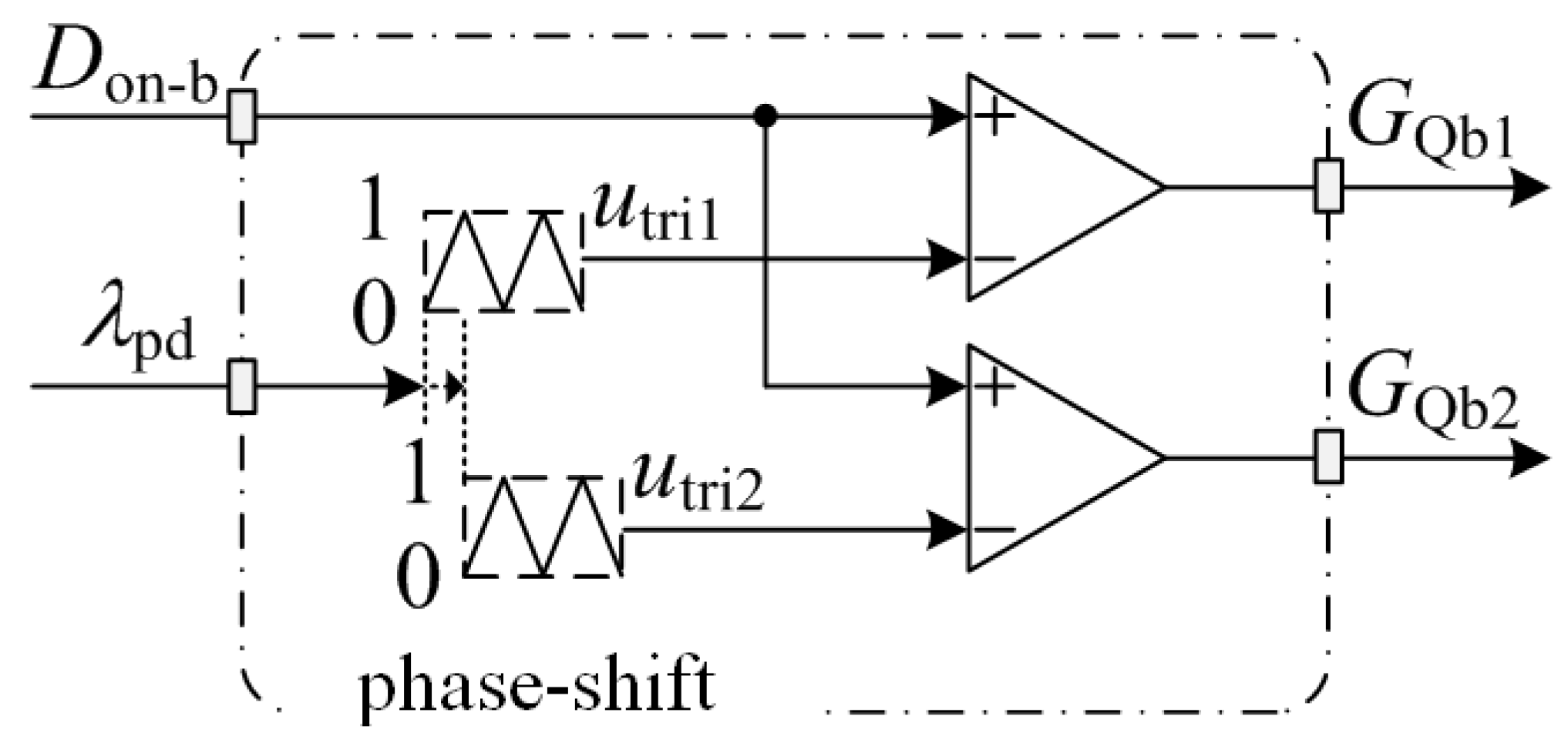
To realize the independent control of the deviation voltage without changing the output characteristics, a pulse phase-shift control strategy for TLBC is proposed in this paper. The independent charging of capacitor can be realized by adjusting the phase difference between two PWM signals G_Qb1 and G_Qb2. Figure 6 shows the pulse generating units of phase-shift control strategy. G_Qb1 and G_Qb2 are both obtained by comparing voltage references with triangle carriers. Two voltage references (D_on-b) are the same, but phase-shift angle λ_pd exists between two carriers $u_{\mathrm{tri}1}$ and $u_{\mathrm{tri}2}$. λ_pd = t_pd/T_sb, where t_pd is the phase-shift time and T_sb is the switching period.

For the conventional control, two carriers have a fixed phase angle (λ_pd = 0.5). Therefore, the effect that the input voltage takes on two filtering capacitors is the same, the midpoint potential of TLBC cannot be regulated actively. However, for the phase-shift control, λ_pd can change from 0 to 1. Further study shows that λ_pd can be divided into different sections, and the deviation voltage ∆u_cb can be eliminated by adjusting the λ_pd [45].

Table 3. Deviation voltage regulating principle of phase shift-control strategy.

Don-b	λpd	Charging Current	Effect on uCb1 and uCb2
Don-b ≤ 0.5	λpd = 0	IuCb1 = IuCb2	no effect
	0 < λpd < 0.5	IuCb1 > IuCb2	Increase uCb1
	λpd = 0.5	IuCb1 = IuCb2	no effect
	0.5 < λpd < 1	IuCb1 < IuCb2	increase uCb2
Don-b > 0.5	λpd = 0	IuCb1 = IuCb2	no effect
	0 < λpd < 0.5	IuCb1 > IuCb2	increase uCb1
	λpd = 0.5	IuCb1 = IuCb2	no effect
	0.5 < λpd < 1	IuCb1 < IuCb2	increase uCb2

shows the deviation voltage regulating principle of the pulse phase-shift control.

It can be seen in Table 3 that no matter what D_on-b the system is in, when the λ_pd is in the range of (0.5, 1), the u_Cb2 will rise. However, when the λ_pd is in the range of (0, 0.5), the u_Cb1 will rise.

For different D_on-b and λ_pd, the transition of basic switching modes in a unit switch period is different. According to this, there will be 10 cases, as shown in

Table 4. Summary table of working condition and mode switch.

Case	Working Condition	Mode Transition
I	λpd = 0	M1→M4
II	Don-b ≤ 0.5, 0 < λpd < Don-b or Don-b > 0.5, 0 < λpd < 1 − Don-b	M2→M1→M3→M4
III	Don-b < 0.5, λpd = Don-b	M2→M3→M4
IV	Don-b < 0.5, Don-b < λpd < 1 − Don-b	M2→M4→M3→M4
V	Don-b < 0.5, λpd = 1 − Don-b	M2→M4→M3
VI	Don-b ≤ 0.5, 1 − Don-b < λpd < 1 or Don-b > 0.5, Don-b < λpd < 1	M1→M2→M4→M3
VII	Don-b = 0.5, λpd = Don-b	M2→M3
VIII	Don-b > 0.5, λpd = 1 − Don-b	M2→M1→M3
IX	Don-b > 0.5, 1 − Don-b < λpd < Don-b	M1→M2→M1→M3
X	Don-b > 0.5, λpd = Don-b	M1→M2→M3

.

To establish a relatively accurate mathematical model to analyze the steady-state and dynamic performance of TLBC, a modeling method based on inductor current ripple is adopted in this paper [44].

Taking Case II as an example, the output voltage gain M_ob and the deviation voltage gain M_eb of the TLBC can be obtained respectively.

$$\{\begin{array}{l}{M}_{\mathrm{ob}}=\frac{V_{\mathrm{ob}}}{V_{\mathrm{dc}}}=\frac{1}{1-D_{\mathrm{on}-\mathrm{b}}}\\ M_{\mathrm{eb}}=\frac{\mathsf{\Delta }{u}_{cb}}{V_{\mathrm{dc}}}=\frac{R_{\mathrm{b}}}{4L_{\mathrm{b}}{f}_{\mathrm{sb}}}{k}_{dc}=\frac{R_{\mathrm{b}}}{4L_{\mathrm{b}}{f}_{\mathrm{sb}}}{\lambda }_{\mathrm{pd}}(\frac{1-D_{\mathrm{on}-\mathrm{b}}-{\lambda }_{\mathrm{pd}}}{1-D_{\mathrm{on}-\mathrm{b}}}+2D_{\mathrm{on}-\mathrm{b}}-1)\end{array}$$

(1)

where k_dc denotes the gain coefficient of deviation voltage.

It can be seen from Equation (1) that M_ob is not affected by λ_pd, but M_eb is determined by both D_on-b and λ_pd. Therefore, it may be found that M_ob is exactly the same, but k_dc is different in some situations. The expression of k_dc in other cases can be obtained by the same modeling method [45], and the three-dimensional surface of k_dc can be plotted as shown in Figure 7. It can be seen that, when λ_pd = 0, 0.5, 1, there will be k_dc = 0, no effect on the deviation voltage; when 0 < λ_pd < 0.5, there will be k_dc > 0, the u_Cb1 will rise; and when 0.5 < λ_pd < 1, there will be k_dc < 0, the u_Cb2 will rise. In Figure 7, there are two extreme points A and B, which means the regulation ability of pulse phase-shift control is limited in a certain range. However, for the application of this paper, there is no independent load for C_b1 and C_b2, the proposed pulse phase-shift control is applicable. In addition, it cannot be considered that the larger or smaller the λ_pd is, the stronger the regulation ability is.

3.4. Verification of MPB Control

To verify the feasibility of the proposed pulse phase-shift control, a 10 kVA prototype experimental platform was built, as shown in Figure 8, whose control system was based on digital signal processor (DSP) and field programmable gate array (FPGA) for digital implementation.

Different resistance loads were used to simulate various midpoint potential shifts of TLBC for improving the flexibility of the experiment. Then, the feasibility of the pulse phase-shift control strategy adopted in this paper was fully verified. The main circuit parameters were: V_dc = 1000 V, V_ob = 1500 V, D_on-b = 1/3, f_sb = 8 kHz, L_b = 1.5 mH, and C_b1 = C_b2 = 2267 μF. Under normal condition, the load resistors were R_b1 = R_b2 = 50 Ω. Then, the two resistors are finely changed to simulate different midpoint potential shifts.

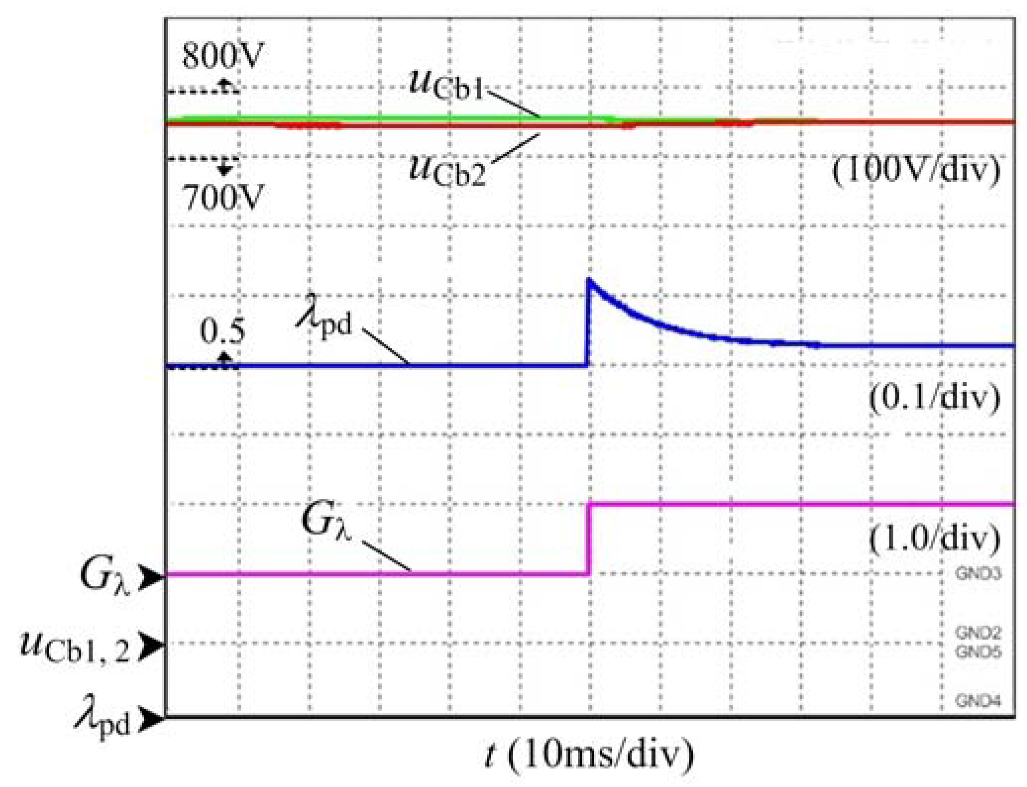
Figure 9 shows the experimental waveforms with and without the proposed MPB control strategy when R_b1 increases from 50 Ω to 52 Ω. In Figure 9, u_cb1 and u_cb2 are two capacitors’ voltages, respectively; λ_pd is the phase shift signal; and G_λ is the enable signal for the midpoint potential balancing control. The increase of R_b1 results in u_cb1 > u_cb2. When G_λ = 0, the MPB control strategy is not enabled and λ_pd is equal to 0.5, so the capacitor voltage deviation occurs, and the deviation voltage stays at 21 V. When G_λ = 1, the MPB control strategy is activated. λ_pd is adjusted to greater than 0.5 to increase u_cb2 and reduce u_cb1, which is consistent with the previous theoretical analysis. The deviation voltage becomes approximately 0 after 30 ms, when λ_pd stays at a value of more than 0.5.

The deviation voltage has a further increase when R_b1 increases from 52 Ω to 54 Ω, as shown in Figure 10. In Figure 10, the deviation voltage increases to 35 V at this time. When the MPB control strategy is enabled, λ_pd rapidly reaches the upper limit 0.78. The adjusting ability at this time is the strongest. Then, λ_pd gradually decreases with the decrease of the deviation voltage, and stays in the value of more than 0.5 after 35 ms later. At last, the deviation voltage goes back to zero.

Similar results can be obtained when R_b1 increases from 54 Ω to 64 Ω. However, the deviation voltage increases to 174 V, and it cannot go back to zero even if the MPB control strategy is enabled, which indicates that the adjusting ability of MPB control is limited.

For the application in PV system, no independent loads are imposed on the two capacitors. The proposed MPB control strategy based on pulse phase-shift should be effective.

4. Reversible Converter

4.1. Main Circuit

The main circuit of reversible converter is shown in Figure 11. It is composed of a multi-winding transformer T and two identical four-quadrant converters (4QC1/4QC2). L is the AC filter inductance of the 4QC, C is the capacitance of DC-Link, $u_{\mathrm{dc}}$ is the DC voltage, $i_{\mathrm{dc}}$ is the DC current, $e_{\mathrm{abc}}$ is the transformer secondary voltage, and $e_{\mathrm{grid}}$ is the AC grid voltage.

Using this multi-modular topology, the capacity of the converter can be enlarged and the reliability can be improved. The phase-shift carrier PWM technology can be used to reduce the harmonics of the AC grid current and improve the power quality [41].

4.2. Current Decoupling Control

According to KVL law, the mathematic model of the 4QC can be given in Equation (2).

$$\{\begin{array}{c}{e}_{\mathrm{a}}=L\frac{d{i}_{\mathrm{a}}}{dt}+u_{\mathrm{a}}\\ e_{\mathrm{b}}=L\frac{d{i}_{\mathrm{b}}}{dt}+u_{\mathrm{b}}\\ e_{\mathrm{c}}=L\frac{d{i}_{\mathrm{c}}}{dt}+u_{\mathrm{c}}\end{array}$$

(2)

where: $e_{\mathrm{a}},e_{\mathrm{b}},e_{\mathrm{c}}$ is the phase voltage of the grid; $i_{\mathrm{a}},i_{\mathrm{b}},i_{\mathrm{c}}$ is the current of each phase; $u_{\mathrm{a}},u_{\mathrm{b}},u_{\mathrm{c}}$ is the phase voltage of 4QC.

Using abc/dq transformation matrix, Equation (2) can be written as:

$$\{\begin{array}{c}{e}_{\mathrm{d}}=L\frac{d{i}_{\mathrm{d}}}{dt}-\omega L{i}_{\mathrm{q}}+u_{\mathrm{d}}\\ e_{\mathrm{q}}=L\frac{d{i}_{\mathrm{q}}}{dt}+\omega L{i}_{\mathrm{d}}+u_{\mathrm{q}}\end{array}$$

(3)

The control voltage under dq frame can be calculated by Equation (4):

$$\{\begin{array}{c}{u}_{\mathrm{d}}=-L\frac{d{i}_{\mathrm{d}}}{dt}+\omega L{i}_{\mathrm{q}}+e_{\mathrm{d}}\\ u_{\mathrm{q}}=-L\frac{d{i}_{\mathrm{q}}}{dt}-\omega L{i}_{\mathrm{d}}+e_{\mathrm{q}}\end{array}$$

(4)

Finally, closed-loop control block for AC current of each 4QC is shown in Figure 12. AC current control is the foundation of the reversible converter control, because it has an important influence on the current waveform, total harmonic distortion(THD), power factor and dynamic response.

5. Working Characteristic and Coordinate Control

5.1. Working Characteristics

5.1.1. Twelve-Pulse Rectifier

A 12-pulse rectifier can be represented by an ideal DC voltage source U_k in series with an internal resistance R_eq and a diode D as Equation (5).

$$U_{\mathrm{dc}}=U_{\mathrm{k}}-R_{\mathrm{eq}}{I}_{\mathrm{dc}}$$

(5)

The DC output characteristic curve of a 12-pulse rectifier is shown in Figure 13. The critical current (or transition current) I_dg is bounded. The curve is divided into two curves: ① is the curve that two six-pulse rectifiers work in a push-pull mode; and ② the curve that two six-pulse rectifiers work in parallel. U_k denotes the no-load voltage of a six-pulse rectifier, U_dN denotes the rated output voltage of a 12-pulse rectifier, and I_dN denotes the rated output voltage of a 12-pulse rectifier.

The equivalent resistance R_eq varies with the load current and can be expressed as Equation (6).

$$R_{\mathrm{eq}}=\{\begin{array}{l}\frac{3X_{\mathrm{c}}}{\pi }，\mathrm{when}0<I_{\mathrm{dc}}<I_{\mathrm{dg}}\\ \frac{3X_{\mathrm{c}}}{2\pi }，\mathrm{when}{I}_{\mathrm{dg}}<I_{\mathrm{dc}}<I_{\mathrm{dN}}\end{array}$$

(6)

where X_c is the short-circuit impedance of TR.

5.1.2. Reversible Converter

In the proposed power supply system, reversible converter set can be used to recover the surplus regenerative braking energy, as well as to power the train. It has the notable features of bidirectional power flow and controllable DC output characteristic. The DC output characteristic is shown in Figure 14. In Figure 14, the inverting area is located in the second quadrant (left), and the rectifying area is located in the first quadrant (right). AD and AB are defined as constant voltage curve. The 4QC can be equal to an ideal voltage source, and the corresponding maximum operating current are $I_{\mathrm{dn}}^{+}$ and $I_{\mathrm{dn}}^{-}$, respectively. BC and DE are defined as constant power curves, and the 4QC can be equal to ideal power source. Regarding the curve BC, due to the limitation of rectifying power $P_{\mathrm{rec}}^{\max }$, the 4QC DC output voltage will rapidly drop with the increase of the train traction power, following the law of hyperbola. Considering the curve DE, because of the limitation of inverting power $P_{\mathrm{inv}}^{\max }$, the 4QC DC output voltage will rapidly rise with the increase of the train braking power, following the law of hyperbola. In general, $\left|P_{\mathrm{rec}}^{\max }\right|=\left|P_{\mathrm{inv}}^{\max }\right|=P_{\max }$, where P_max denotes the maximum power of the converter.

The DC voltage characteristics of 4QC can be expressed by Equation (7).

$$u_{\mathrm{dc}}=\{\begin{array}{l}{U}_{\mathrm{dn}},\mathrm{when}{I}_{\mathrm{dn}}^{-}\le I_{\mathrm{dc}}\ll I_{\mathrm{dn}}^{\mp }\\ \frac{P_{\mathrm{rec}}^{\max }}{i_{\mathrm{dc}}},\mathrm{when}{I}_{\mathrm{dn}}^{+}<I_{\mathrm{dc}}\\ \frac{P_{\mathrm{inv}}^{\max }}{i_{\mathrm{dc}}},\mathrm{when}{I}_{\mathrm{dc}}<I_{\mathrm{dn}}^{-}\end{array}$$

(7)

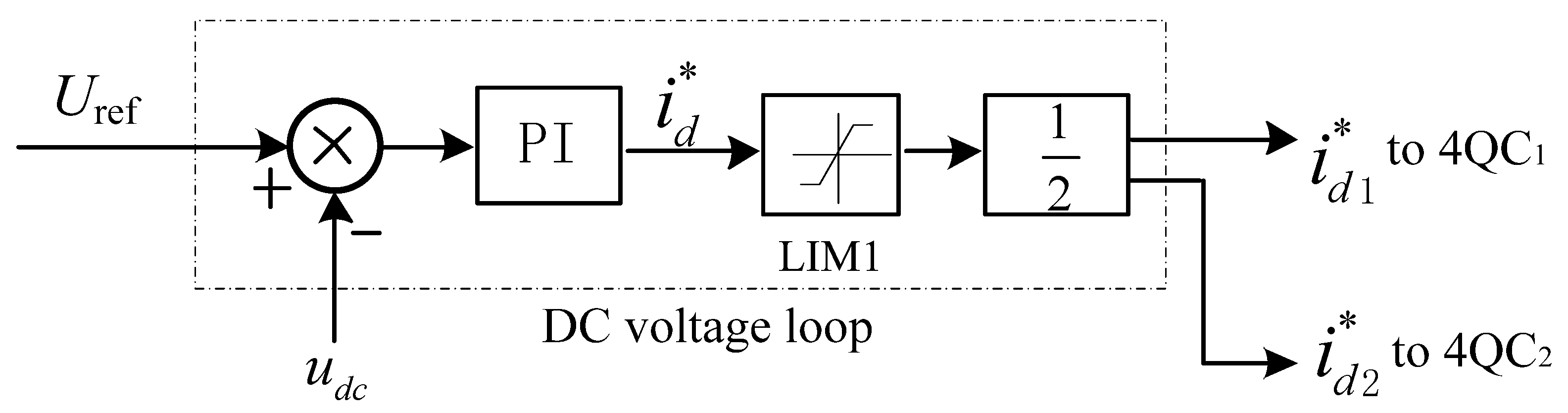
Since there are two 4QC units in a reversible converter system, a DC voltage control scheme is proposed in Figure 15, which makes the traction substation has the expected DC characteristic as shown in Figure 14, also ensure two 4QCs share the load equally.

In Figure 15, the output of PI controller $\left(i_{\mathrm{d}}^{\ast }\right)$ indicates the total active power demand. LIM1 is the active power limitation block, whose maximum value $i_{\mathrm{d}}^{\max }$ can be calculated by:

$$\left|i_{\mathrm{d}}^{\max }\right|=\frac{S}{\frac{3}{2}{e}_{\mathrm{d}}}$$

(8)

where S denotes the capacity of the reversible converter set, $e_{\mathrm{d}}$ denotes AC voltage of 4QC in dq frame (when $e_{\mathrm{q}}=0$).

5.1.3. PV System

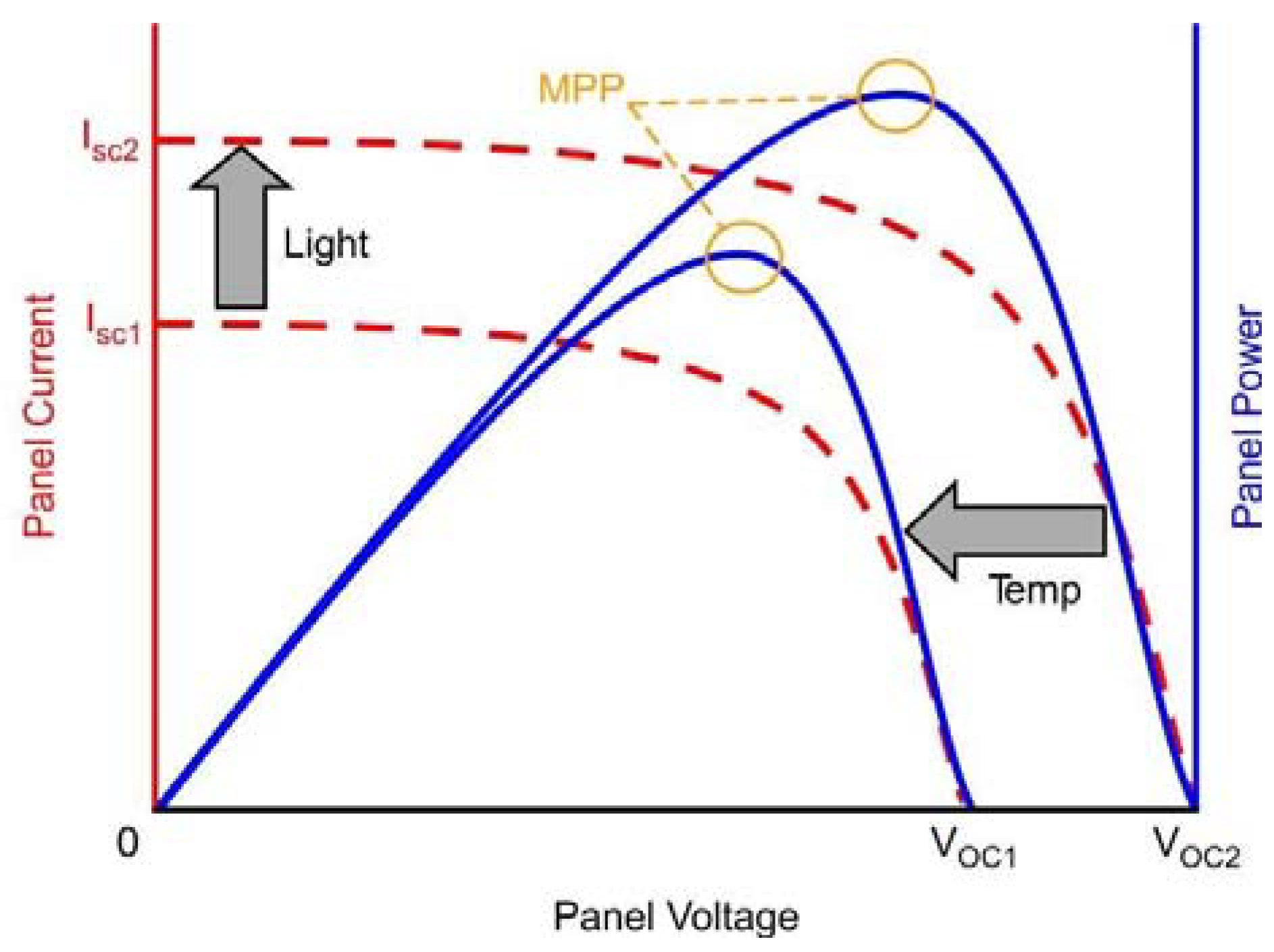
Besides the midpoint potential balancing control, TLBC need to achieve the maximum capture of solar energy and transfers it to the DC network. For the HTPSS, it can be equivalent to a variable power source with fixed energy direction. The output power of PV system P_pv is related to the characteristics of the solar panels (as shown in Figure 16) [46], which is mainly influenced by panel cell temperature and irradiation levels. Suppose the efficiency of TLBC is 1, Equation (9) can be obtained.

$$P_{\mathrm{pv}}=f\left(T_{\mathrm{c}},J_{\mathrm{ir}}\right){|}_{\max }$$

(9)

where T_c denotes panel cell temperature and J_ir denotes irradiation levels.

It is worth noting that PV system can also be regarded as a constant power source at a certain time point or in a short time period.

5.2. Coordinated Control Strategy

Figure 17 shows the equivalent model of the HTPSS with one traction substation and one train, where DR denotes 12-pulse rectifier, RC denotes reversible converter, PV denotes the PV system, and TR denotes train. The reversible converter is equivalent to the combination of constant voltage source and power source, and the train is equivalent to a bidirectional power source.

To guarantee good performance of traction power supply and take into account the maximum economic benefits of PV system, the following principles should be considered.

Principle 1: Dynamic capacity distribution of RC

When the required active power exceeds the rated capacity, the reversible converter runs at rated power, and DC voltage is uncontrollable. When the required active power is less than the rated capacity, the reversible converter can keep the DC voltage constant by adjusting the active power. In addition, the residual capacity can be used as reactive power compensation to improve the power factor of medium voltage ring network.

According to the instantaneous power theory:

$$\{\begin{array}{l}P=\frac{3}{2}{e}_{\mathrm{d}}{i}_{\mathrm{d}}+\frac{3}{2}{e}_{\mathrm{q}}{i}_{\mathrm{q}}\\ Q=\frac{3}{2}{e}_{\mathrm{d}}{i}_{\mathrm{q}}+\frac{3}{2}{e}_{\mathrm{q}}{i}_{\mathrm{d}}\\ S^2=P^2+Q^2\end{array}$$

(10)

where S denotes the apparent power, P and Q denote the active power and reactive power, $e_{\mathrm{d}}$ and $e_{\mathrm{q}}$ denote the grid voltage, and $i_{\mathrm{d}}\mathrm{and}{i}_{\mathrm{q}}$ denote the active and reactive current.

Considering $e_{\mathrm{q}}=0$

$$i_{\mathrm{q}}^{\max }=\frac{\sqrt{S^2-P^2}}{\frac{3}{2}{e}_{\mathrm{d}}}$$

(11)

The dynamic distribution diagram of active and reactive power is shown in Figure 18. LIM2 is a reactive power limiting unit. The maximum allowable reactive current value of the reversible converter is calculated through Equation (11) and passed to LIM2.

Principle 2: Dynamic power limitation for PV

When DC network voltage is under the threshold U_d1, TLBC should do its best to transmit solar power to DC network. However, the transmitted power will be limited when DC network voltage exceeds the threshold U_d1, as shown in Equation (12).

$$P_{\mathrm{tlbc}}=\{\begin{array}{cc}{P}_{\mathrm{pv}},\hfill & \mathrm{when}{U}_{\mathrm{dc}}\ll U_{\mathrm{d}1}\hfill \\ \frac{U_{\mathrm{d}2}-U_{\mathrm{dc}}}{U_{\mathrm{d}2}-U_{\mathrm{d}1}}\times P_{\mathrm{pv}},\hfill & \mathrm{when}{U}_{\mathrm{d}1}<U_{\mathrm{dc}}\ll U_{\mathrm{d}2}\hfill \\ 0,\hfill & \mathrm{when}{U}_{\mathrm{d}2}<U_{\mathrm{dc}}\hfill \end{array}$$

(12)

where $U_{\mathrm{d}1}\mathrm{and}{U}_{\mathrm{d}2}$ are the voltage threshold, and $P_{\mathrm{pv}}$ is the output power of the solar panels.

Principle 3: Voltage match between DR and RC

When the DC network voltage is lower than the ideal no-load voltage U_k, the diode rectifier will begin to supplement the power required by the train and ensure the reliability of power supply. Meanwhile, to prevent circulation between diode rectifier unit and reversible converter, Equation (13) should be met.

$$U_{\mathrm{k}}\le U_{\mathrm{dn}}-\mathsf{\Delta }\mathrm{V}$$

(13)

where $U_{\mathrm{dn}}$ is the rated DC voltage of reversible converter and $\mathsf{\Delta }\mathrm{V}$ is the anti-circulating voltage threshold (normally 30–50 V).

Principle 4: Characteristic match between TR and PV

The train can be modeled as a time-varying power source, whose value is normally determined by the train running state. However, when the DC voltage exceeds the threshold U_d3, regenerative braking power of the train needs to be linearly reduced, until DC voltage reaches the threshold U_d4, the regenerative braking becomes zero. In this way, the further rise of the DC network voltage can be avoided. Meanwhile, to make full use of train’s regenerative braking capability, TLBC needs to reduce power to zero before the DC network voltage rises to U_d3. The interrelation is shown in Equation (14).

$$U_{\mathrm{d}1}<U_{\mathrm{d}2}\le U_{\mathrm{d}3}<U_{\mathrm{d}4}$$

(14)

5.3. Simulation Verification

5.3.1. System Parameters

To verify the effectiveness of the coordinate control algorithm, a system simulation model containing a traction substation and a train is built in Matlab/Simulink, and several typical working conditions are simulated and verified. The simulation system is shown in Figure 19.

The system parameters are shown in

Table 5. Parameters in the case study.

Item	Parameters	Value
110 kV and 35 kV AC cable	Resistance per unit length (Ω/km)	0.158
	Inductance per unit length (mH/km)	0.287
	Capacitance per unit length (μF/km)	0.156
12-pulse diode rectifier	Rated capacity (MW)	2
	Input AC voltage (kV)	35
	No-load DC voltage Uk (V)	1650
	Transformer short-circuit resistance (%)	8%
TLBC	Rated capacity (MW)	1
	AC filtering inductor Lb (mH)	1
	DC-Link capacitor Cb1/Cb2 (mF)	3
	Switch frequency (kHz)	4
	Threshold Ud1, Ud2 (V)	1800, 1900
Reversible converter	AC input rated voltage (kV)	35
	DC rated voltage Udn (V)	1700
	Rated capacity (MVA)	2 × 1
	AC filtering inductor L (μH)	150
	DC-Link capacitor C (mF)	36
	Switch frequency (kHz)	2
Train	Maximum traction power (MW)	4
	Maximum braking power (MW)	−3.5
	Threshold Ud3, Ud4 (V)	1900, 2000

.

5.3.2. Case Study 1

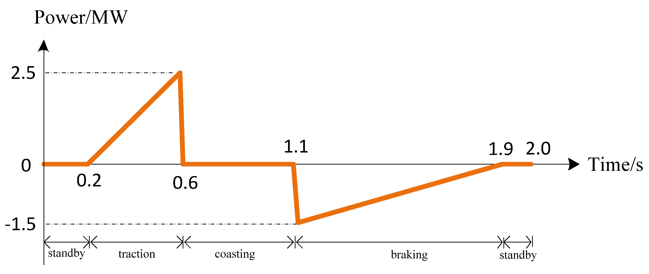
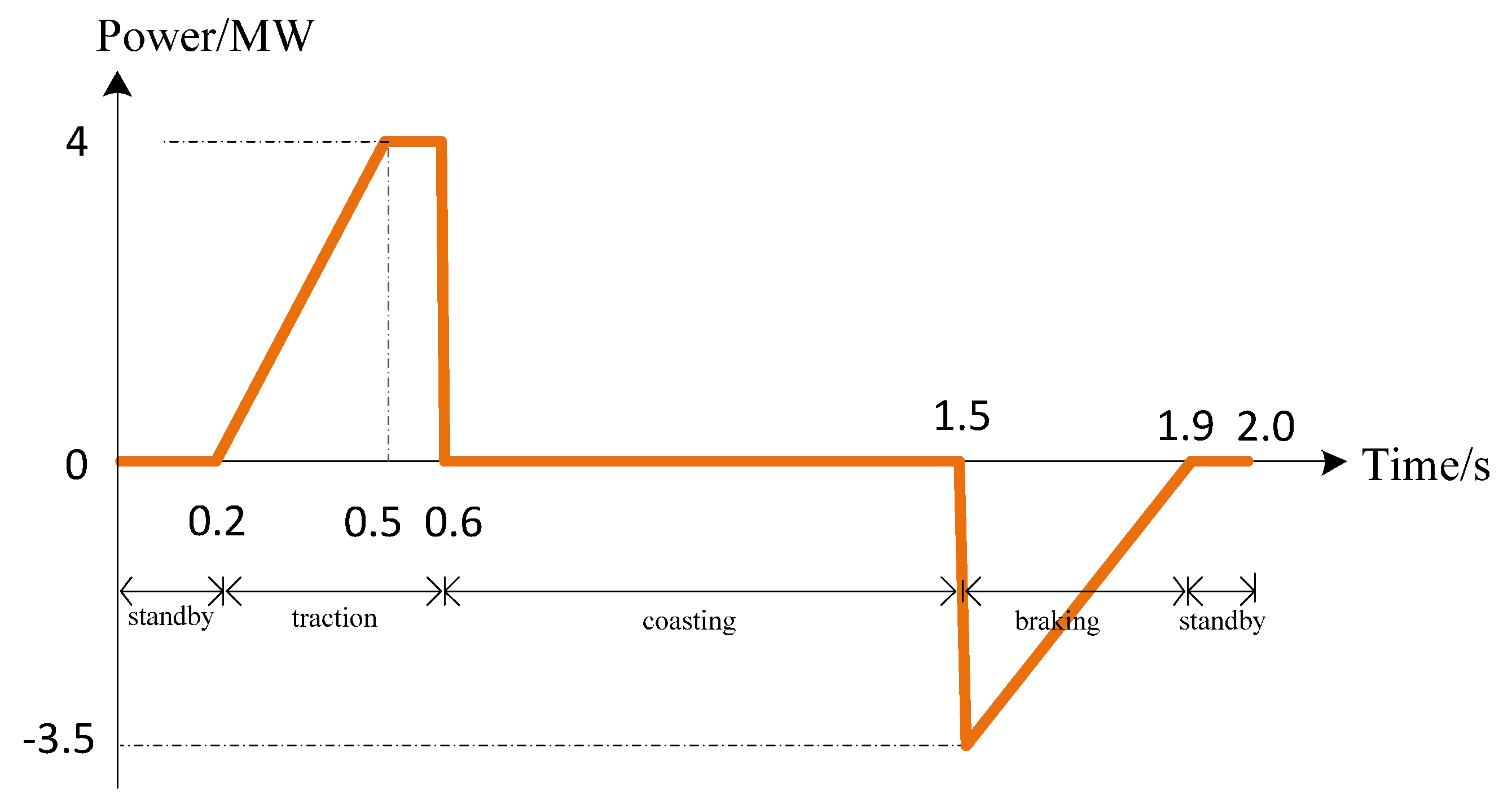
The output power of the PV is constant 1 MW, and the reactive power compensation of the reversible converter is not enabled. The peak traction power and braking power of the train reaches 2.5 MW and −1.5 MW, respectively. The power curve of the train is shown in Figure 20.

Figure 21 shows the DC voltage and power curve obtained by simulation. The reversible converter has been working in an inverting state with a power of −1 MW before t = 0.2 s. The traction power required by train begins to increase from t = 0.2 s. The output power of PV keeps constant 1 MW. The work state of the reversible converter changes from inverting state to rectifying state at Point A, from which it begins to provide traction energy for the train. The train switches to coasting state at t = 0.6 s, the required power is rapidly reduced, and so the output power of the reversible converter is reduced. The reversible converter changes to inverting state at Point B and begins to invert the PV power back to the grid once more. The train begins to brake at t = 1.1 s, and the braking power increases rapidly, making the inverting power of the reversible converter increase fast from −1 MW to −2 MW (Point C), and then kept at −2 MW after a short transient process. Because the sum of the PV’s power and train’s braking power is greater than the inverting capacity of the reversible converter, the DC voltage starts to rise (Point D). When the DC voltage reaches 1800 V (Point E), the PV begins to actively reduce the output power (Point F) until the power balance is reached (Point G) and the DC voltage gets to the peak. Then, as the braking power of the train decreases, the DC voltage starts to fall, and the PV power begins to increase gradually. The reversible converter keeps working at rated power during this period. Until Point H, the output power begins to decrease, and finally returns to −1 MW at t = 1.9 s (Point I). During the whole period, the output power of the diode rectifier is always zero, and the DC voltage shows good controllability when the reversible converter is within its power limit.

Figure 22 shows the current reference and the obtained waveforms of the reversible converter. During the periods [0, 0.2], [0.6, 1.1] and [1.9, 2.0], the current reference of 4QC1 is kept at $i_{\mathrm{d}1}^{\ast }=-0.5$, and the corresponding power is −1 MW. During the rest of the time, $i_{\mathrm{d}1}^{\ast }$ changes with the running state of the train, and the amplitude of $i_{\mathrm{a}}$ has the same changing law as $i_{\mathrm{d}1}^{\ast }$.

Due to phase-shift carrier PWM technology, most of the harmonics of 4QC1 and 4QC2 near the switching frequency f_s can be eliminated, thus reducing the current harmonic content injected into the grid. At the instant t = 1.3 s, the THD of the AC current injected into 35 kV grid is 3.06%; the FFT analysis result is shown in Figure 23.

5.3.3. Case Study 2

The output power of the PV is constant 1 MW, and the reactive power compensation of reversible converter is not enabled. The peak traction power and braking power of the train reaches 2.5 MW and −1.5 MW, respectively. The power curve is shown in Figure 24.

Figure 25 shows the DC voltage and power curve in Case 2 obtained by simulation. It can be seen that, when the limit power of the reversible converter is reached (Point B), the DC voltage begins to decline at Point C. When the DC voltage drops below the no-load voltage 1650 V of the 12-pulse rectifier (at Point D), the 12-pulse rectifier starts to work (Point E). It provides traction energy to the train and discourages the further drop of the DC voltage. The train switches to coasting state at t = 0.6 s, the required power is rapidly reduced to zero, so the output power of 12-pulse rectifier decreases to zero, and the reversible converter changes to inverting state. The train begins to brake at t = 1.5 s, and the braking power increases rapidly, making the inverting power of the reversible converter increase fast from −1 MW to −2 MW, and then kept at −2 MW after a short transient process. As the sum of the PV’s power and train’s braking power is greater than the inverting capacity of the reversible converter, the DC voltage starts to rise at Point F. When the DC voltage reaches 1800 V (Point G), the PV begins to actively reduce the output power from Point H. Because the train braking power is too high, the DC voltage is still rising rapidly. Until it reaches 1900 V (Point I), the braking power of the train has to decline linearly with the rise of the DC voltage. When the braking power decrease to −2 MW, the power balance between the train and reversible converter has been realized. After that, as the train speed decreases, the braking power falls to below −2 MW at Point J. When DC voltage comes down to 1900 V (Point K), the output power of PV begins to increase (Point L), until the rated power 1 MW is recovered (Point M). Finally, the train stops at t = 1.9 s and the reversible converter comes back to −1 MW (Point N).

Figure 26 shows the current reference and the obtained waveforms of the reversible converter. It can be seen that $i_{\mathrm{a}}$ and $e_{\mathrm{a}}$ remain the same phase or opposite phase, and the amplitude of $i_{\mathrm{a}}$ has the same changing law as $i_{\mathrm{d}1}^{\ast }$.

5.3.4. Case Study 3

In this case, the train runs according to power curve shown in Figure 20. Suppose it is the time after sunset, so output power of the PV system is zero. Assume that the length of 35 kV and 110 kV cables is about 2 km, and the auxiliary load of the substation is 200 kW.

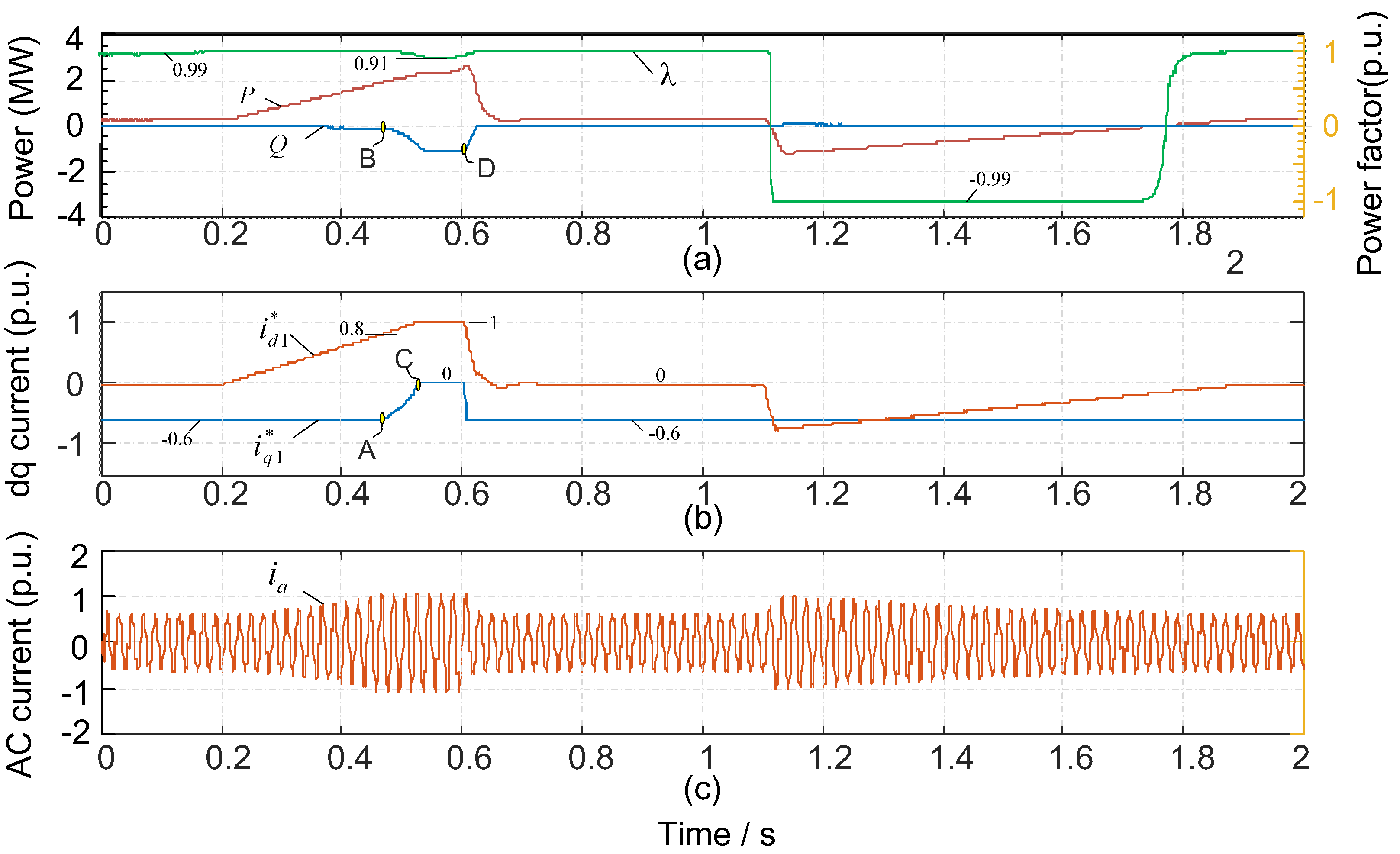
Figure 27 shows the curves of active power, reactive power and power factor without reactive power compensation. It can be seen that the reactive power Q generated by equivalent capacitance of AC cable is about 1.2 MVar, and the power factor λ is as low as about 0.2 when the train is in coasting or standby state. It is worth noting that the reversible converter is in the standby state during this period.

Figure 28 shows the curves of active power, reactive power and power factor with reactive power compensation. It can be seen that, with a given reference $i_{\mathrm{q}1}^{\ast }=-0.6$, a good compensation effect can be obtained. The system power factor λ at the interface of the power company is improved up to 0.99. However, with the increase of the train power, the reactive current reference $i_{\mathrm{q}1}^{\ast }$ begins to reduce at Point A when $i_{\mathrm{d}1}^{\ast }$ reaches 0.8. The reactive power Q begins to increase from Point B. The system power factor λ gradually drops to 0.91. When t = 0.6 s, the train switches to coasting mode, $i_{\mathrm{d}1}^{\ast }$ begins to decline rapidly, so the reactive current reference $i_{\mathrm{q}1}^{\ast }$ starts to recover, and the reactive power compensation begins to increase. By means of dynamic distribution of the active and reactive power, the residual capacity of the reversible converter can be used to improve the system power factor, replacing the special SVG equipment.

The feasibility and effectiveness of the proposed HTPSS and corresponding coordinated control strategy have been verified by above simulations. The reversible converter has multiple functions, by which a high utilization rate of the equipment can be achieved and the investment payback period can be shortened. Owing to the confined spatial, the detailed economic benefit evaluation of the system under multi-train operation scenario have not been included in this paper.

6. Conclusions

A novel hybrid traction power supply system is constructed by introducing PV and reversible converter in this paper. Three-level boost converter is employed as the DC/DC converter in the PV system. A midpoint potential balancing control method based on pulse phase-shift is presented, and then verified by a prototype experiment. The reversible converter is based on multi-modular topology. A current decoupling control scheme based on dq frame has been adopted to achieve independent regulation of active and reactive power. Based on the comprehensive study of the working characteristics, a system coordinated control strategy is proposed, and four cooperative principles are given out. The simulation results under multi-working conditions verified the effectiveness of the topology and coordinated control strategy of the proposed HTPSS.

The optimal configuration for the capacity of PV system and reversible converter will be studied in the future.

References

- Jabr, R.A.; Džafić, I. Solution of DC Railway Traction Power Flow Systems Including Limited Network Receptivity. IEEE Trans. Power Syst. 2018, 33, 962–969. [Google Scholar] [CrossRef]
- Tian, Z.; Hillmansen, S.; Roberts, C.; Weston, P. Energy evaluation of the power network of a DC railway system with regenerating trains. IET Electr. Syst. Transp. 2015, 6, 41–49. [Google Scholar] [CrossRef]
- Zhu, Z. Research on Reactive Power Compensation Scheme and Compensation Capacity of Subway Power Supply System. World Invert. 2014, 11, 45–47. [Google Scholar]
- Reza, S.; Azah, M.; Shareef, H. Comparative study of effectiveness of different var compensation devices in large-scale power networks. J. Cent. South Univ. 2013, 3, 715–723. [Google Scholar]
- Liu, R.; Liu, W.; Cui, H.; Zhang, J.; Liao, J. Capacity optimization design of reactive compensation device in urban rail traction power supply system. In Proceedings of the 2017 IEEE Transportation Electrification Conference and Expo, Chicago, IL, USA, 22–24 June 2017; pp. 1–6. [Google Scholar]
- Yii, S.T.; Ruay-Nan, W.; Nanming, C. Electric network solutions of DC transit systems with inverting substations. IEEE Trans. Veh. Technol. 1998, 47, 1405–1412. [Google Scholar]
- Mellitt, B.; Mouneimne, Z.S.; Goodman, C.J. Simulation study of DC transit systems with inverting substations. Electr. Power Appl. 1984, 131, 38–50. [Google Scholar] [CrossRef]
- Suzuki, T. DC power-supply system with inverting substations for traction systems using regenerative brakes. Electr. Power Appl. 1982, 129, 18–26. [Google Scholar] [CrossRef]
- Serrano-Jiménez, D.; Abrahamsson, L.; Castaño-Solís, S.; Sanz-Feito, J. Electrical railway power supply systems: Current situation and future trends. Int. J. Electr. Power Energy Syst. 2017, 92, 181–192. [Google Scholar] [CrossRef]
- Ghaviha, N.; Campillo, J.; Bohlin, M.; Dahlquist, E. Review of Application of Energy Storage Devices in Railway Transportation. Energy Procedia 2017, 105, 4561–4568. [Google Scholar] [CrossRef]
- Jandura, P.; Richter, A.; Ferkov, Z. Flywheel energy storage system for city railway. In Proceedings of the 2016 International Symposium on Power Electronics, Electrical Drives, Automation and Motion, Anacapri, Italy, 22–24 April 2016; pp. 1155–1159. [Google Scholar]
- Douglas, H.; Roberts, C.; Hillmansen, S.; Schmid, F. An assessment of available measures to reduce traction energy use in railway networks. Energy Convers. Manag. 2015, 106, 1149–1165. [Google Scholar] [CrossRef]
- González-Gil, A.; Palacin, R.; Batty, P. Sustainable urban rail systems: Strategies and technologies for optimal management of regenerative braking energy. Energy Convers. Manag. 2013, 75, 374–388. [Google Scholar] [CrossRef]
- Gelman, V. Braking energy recuperation. IEEE Veh. Technol. Mag. 2009, 4, 82–89. [Google Scholar] [CrossRef]
- Casals, M.; Gangolells, M.; Forcada, N.; Macarulla, M.; Giretti, A. A breakdown of energy consumption in an underground station. Energy Build. 2014, 78, 89–97. [Google Scholar] [CrossRef] [Green Version]
- Kabir, E.; Kumar, P.; Kumar, S.; Adelodun, A.A.; Kim, K. Solar energy: Potential and future prospects. Renew. Sustain. Energy Rev. 2018, 82, 894–900. [Google Scholar] [CrossRef]
- Ding, M.; Xu, Z.; Wang, W.; Wang, X.; Song, Y.; Chen, D. A review on China’s large-scale PV integration: Progress, challenges and recommendations. Renew. Sustain. Energy Rev. 2016, 53, 639–652. [Google Scholar] [CrossRef]
- Kaundinya, D.P.; Balachandra, P.; Ravindranath, N.H. Grid-connected versus stand-alone energy systems for decentralized power—A review of literature. Renew. Sustain. Energy Rev. 2009, 13, 2041–2050. [Google Scholar] [CrossRef]
- Sansaniwal, S.K.; Sharma, V.; Mathur, J. Energy and energy analyses of various typical solar energy applications: A comprehensive review. Renew. Sustain. Energy Rev. 2018, 82, 1576–1601. [Google Scholar] [CrossRef]
- Hayashiya, H.; Furukawa, T.; Itagaki, H.; Kuraoka, T.; Morita, Y.; Fukasawa, Y.; Mitoma, Y.; Oikawa, T. Potentials, peculiarities and prospects of solar power generation on the railway premises. In Proceedings of the 2012 International Conference on Renewable Energy Research and Applications, Nagasaki, Japan, 11–14 November 2012. [Google Scholar]
- Hayashiya, H.; Kikuchi, S.; Matsuura, K.; Hino, M.; Tojo, M.; Kato, T.; Ando, M.; Oikawa, T.; Kamata, M.; Munakata, H. Possibility of energy saving by introducing energy conversion and energy storage technologies in traction power supply system. In Proceedings of the 2013 15th European Conference on Power Electronics and Applications (EPE), Lille, France, 2–6 September 2013; pp. 1–8. [Google Scholar]
- Wang, W.; Wu, M.; Li, Q.; Chen, W. Method for improving power quality of metro traction power supply system with PV integration. In Proceedings of the 2017 Chinese Automation Congress (CAC), Jinan, China, 20–22 October 2017; pp. 1682–1685. [Google Scholar]
- Ciccarelli, F.; Di Noia, L.; Rizzo, R. Integration of Photovoltaic Plants and Supercapacitors in Tramway Power Systems. Energies 2018, 11, 410. [Google Scholar] [CrossRef]
- Shen, X.J.; Zhang, Y.; Chen, S. Investigation of grid-connected photovoltaic generation system applied for Urban Rail Transit energy-savings. In Proceedings of the 2012 IEEE Industry Applications Society Annual Meeting, Las Vegas, NV, USA, 7–11 October 2012; pp. 1–4. [Google Scholar]
- Danandeh, M.A.; Mousavi, G.S.M. Comparative and comprehensive review of maximum power point tracking methods for PV cells. Renew. Sustain. Energy Rev. 2018, 82, 2743–2767. [Google Scholar] [CrossRef]
- Karami, N.; Moubayed, N.; Outbib, R. General review and classification of different MPPT Techniques. Renew. Sustain. Energy Rev. 2017, 68, 1–18. [Google Scholar] [CrossRef]
- Fathabadi, H. Novel fast dynamic MPPT (maximum power point tracking) technique with the capability of very high accurate power tracking. Energy 2016, 94, 466–475. [Google Scholar] [CrossRef]
- Eull, M.; Preindl, M. Bidirectional three-level DC-DC converters: Sum-difference modeling and control. In Proceedings of the 2017 IEEE Transportation Electrification Conference and Expo (ITEC), Chicago, IL, USA, 22–24 June 2017; pp. 573–578. [Google Scholar]
- Tan, L.; Wu, B.; Yaramasu, V.; Rivera, S.; Guo, X. Effective Voltage Balance Control for Bipolar-DC-Bus-Fed EV Charging Station With Three-Level DC-DC Fast Charger. IEEE Trans. Ind. Electron. 2016, 63, 4031–4041. [Google Scholar] [CrossRef]
- Tampubolon, M.; Lin, W.; Lin, J.; Hsieh, Y.; Chiu, H.; Yamanaka, K.; Hojo, M. A study and implementation of three-level boost converter with MPPT for PV application. In Proceedings of the 2017 IEEE 3rd International Future Energy Electronics Conference and ECCE Asia, Kaohsiung, Taiwan, 3–7 June 2017; pp. 1143–1148. [Google Scholar]
- Kang, H.; Cha, H. A New Nonisolated High-Voltage-Gain Boost Converter with Inherent Output Voltage Balancing. IEEE Trans. Ind. Electron. 2018, 65, 2189–2198. [Google Scholar] [CrossRef]
- Lu, S.; Mu, M.; Jiao, Y.; Lee, F.C.; Zhao, Z. Coupled Inductors in Interleaved Multiphase Three-Level DC/DC Converter for High-Power Applications. IEEE Trans. Power Electron. 2016, 31, 120–134. [Google Scholar] [CrossRef]
- Zorig, A.; Belkheiri, M.; Barkat, S. Control of grid connected photovoltaic system using dual three-level stage conversion. In Proceedings of the 2015 4th International Conference on Electrical Engineering (ICEE), Boumerdes, Algeria, 13–15 December 2015; pp. 1–5. [Google Scholar]
- Dusmez, S.; Hasanzadeh, A.; Khaligh, A. Comparative Analysis of Bidirectional Three-Level DC/DC Converter for Automotive Applications. IEEE Trans. Ind. Electron. 2015, 62, 3305–3315. [Google Scholar] [CrossRef]
- Chen, H.C.; Liao, J.Y. Modified Interleaved Current Sensorless Control for Three-Level Boost PFC Converter With Considering Voltage Imbalance and Zero-Crossing Current Distortion. IEEE Trans. Ind. Electron. 2015, 62, 6896–6904. [Google Scholar] [CrossRef]
- Khaldi, H.S.; Ammari, A.C. Fractional-order control of three level boost DC/DC converter used in hybrid energy storage system for electric vehicles. In Proceedings of the Sixth International Renewable Energy Congress, Sousse, Tunisia, 24–26 March 2015; pp. 1–7. [Google Scholar]
- Vitoi, L.A.; Krishna, R.; Soman, D.E.; Leijon, M.; Kottayil, S.K. Control and implementation of three level boost converter for load voltage regulation. In Proceedings of the 39th Annual Conference of the IEEE Industrial Electronics Society, Vienna, Austria, 10–13 November 2013; pp. 561–565. [Google Scholar]
- Xia, C.; Gu, X.; Shi, T.; Yan, Y. Neutral-Point Potential Balancing of Three-Level Inverters in Direct-Driven Wind Energy Conversion System. IEEE Trans. Energy Convers. 2011, 26, 18–29. [Google Scholar] [CrossRef]
- Krishna, R.; Soman, D.E.; Kottayil, S.K.; Leijon, M. Pulse delay control for capacitor voltage balancing in a three-level boost neutral point clamped inverter. IET Power Electron. 2015, 8, 268–277. [Google Scholar] [CrossRef]
- Zhang, G.; Qian, J.; Zhang, X. Application of a High-Power Reversible Converter in a Hybrid Traction Power Supply System. Appl. Sci. 2017, 7, 282. [Google Scholar] [CrossRef]
- Singh, J.; Dahiya, R.; Saini, L.M. Recent research on transformer based single DC source multilevel inverter: A review. Renew. Sustain. Energy Rev. 2018, 82, 3207–3224. [Google Scholar] [CrossRef]
- Rocabert, J.; Luna, A.; Blaabjerg, F.; Rodríguez, P. Control of Power Converters in AC Microgrids. IEEE Trans. Power Electron. 2012, 27, 4734–4749. [Google Scholar] [CrossRef]
- Elsayed, A.T.; Mohamed, A.A.; Mohammed, O.A. DC microgrids and distribution systems: An overview. Electr. Power Syst. Res. 2015, 119, 407–417. [Google Scholar] [CrossRef]
- Du, H. Output Optimization and Efficiency Improvement of High-Frequency Pulsating DC-Link Auxiliary Inverter. Ph.D. Thesis, Beijing Jiaotong University, Beijing, China, 2016. [Google Scholar]
- Zhang, G.; Du, H.; Chen, Y.; Liu, Z. A Midpoint Potential Balance Control Strategy Based on Pulse Phase Delays of Three-level Boost Converter. Proc. CSEE 2017, 20, 6050–6058. [Google Scholar]
- Saravanan, S.; Ramesh Babu, N. Maximum power point tracking algorithms for photovoltaic system—A review. Renew. Sustain. Energy Rev. 2016, 57, 192–204. [Google Scholar] [CrossRef]
Figure 1.
Topology of the hybrid traction power supply system.
Figure 2.
Operating modes of the HTPSS: (a) ; (b) ; (c) ; (d) ; (e) ; (f) ; (g) ; (h) SVG mode; (i) fault mode.
Figure 3.
Main circuit of TLBC.
Figure 4.
Four basic switching modes (M1–M4).
Figure 5.
Control scheme of TLBC.
Figure 6.
Pulse generating units of pulse phase-shift control.
Figure 7.
Three-dimension surface of the deviation voltage gain with pulse phase-shift control.
Figure 8.
Experiment platform of the system.
Figure 9.
Experimental waveforms of the system with and without pulse phase-shift control.
Figure 10.
Figure 11.
Main circuit of the reversible converter.
Figure 12.
Closed-loop control block of AC current.
Figure 13.
Twelve-pulse rectified output characteristic curve.
Figure 14.
Output characteristic curve.
Figure 15.
DC voltage control scheme.
Figure 16.
Typical characteristic of the solar panels.
Figure 17.
Equivalent model of the power supply system.
Figure 18.
Dynamic distribution diagram of the active and reactive power.
Figure 19.
A schematic diagram of the simulation system.
Figure 20.
Power curve of the train in Case 1.
Figure 21.
DC voltage and power curve in Case 1.
Figure 22.
Current reference and obtained waveforms in Case 1.
Figure 23.
Spectrum of the AC current at t = 1.3 s.
Figure 24.
Power curve of the train in Case 2.
Figure 25.
DC voltage and power curve in Case 2.
Figure 26.
Current reference and obtained waveforms in Case 2.
Figure 27.
Curves of reversible converter without reactive power compensation.
Figure 28.
Curves of reversible converter with reactive power compensation.