Abstract
Hydraulic fracturing has been applied in the cave mining industry with the purpose of re-creating an orebody rock mass condition that is suitable for caving. Prescribed hydraulic fracturing was proposed in a previous study as a supplement to the conventional hydraulic fracturing strategy. In this paper; dimensional analysis is used to project laboratory scale numerical modelling results to field scales in order to study the applicability of creating prescribed hydraulic fractures (PHFs) under field conditions. The results indicate that field scale PHFs are feasible if the stress shadows of the pre-located fractures are properly utilized. Water can be used to create the pre-located fractures that induce the local stress change in a low differential stress state; and the use of more proppants and a shorter pre-located fracture spacing lead to PHFs propagating more quickly towards the pre-located fractures. For field condition having high differential stresses, more viscous fluid must be used to create the pre-located fractures in order to enhance the stress shadows. In this case, a shorter pre-located fracture spacing does not necessarily result in the re-orientation of PHFs towards the pre-located fractures and may even lead to unsatisfactory pre-conditioning. A sufficiently high pre-located fracture net pressure to the differential stress ratio (close to 0.5) is the prerequisite for creating PHFs.
1. Introduction
Hydraulic fracturing was invented in the 1940s and its first two commercial trials were realized by the Halliburton Oil Well Cementing Company in Oklahoma and Texas, respectively, in 1949 []. Since then, this technique has been introduced into other industries for various purposes, such as improving gas production in the shale gas industry [] and generating additional flow paths in enhanced geothermal systems []. It has also been used for coal gas drainage for safe mining of coal. This paper focuses on the application of hydraulic fracturing in the metalliferous cave mining industry as an orebody rock mass pre-conditioning method []. Hydraulic fractures (HFs) are generally classified into two types, namely axial HFs and transverse HFs.
The axial HF is assumed to have a rectangular shape in most theoretical studies [,,], and its propagation plane is parallel to the borehole axis. This HF type is common in the oil industry. In practice, the axial HF approximates to an elliptical shape with its short axis perpendicular to bedding planes in sedimentary and metamorphic rocks [].
The transverse HF is also called the penny-shaped HF in some literature [,,] as it is thought to be radial in theoretical analysis [,]. The transverse HF propagates perpendicular to the borehole axis.
The HFs used to pre-condition an orebody rock mass or re-activate a stalled cave back in cave mining are the transverse types. Conventional HFs propagate perpendicular to the minimum in-situ principal stress direction []. He et al. [] discussed the state of the art of cave mining hydraulic fracturing and established the requirement for creating HFs that are not perpendicular to the minimum in-situ principal stress orientation in some geotechnical conditions. This is vital for ensuring that HFs form an additional joint set to increase the probability of achieving a blocky rock mass to improve caveability. These HFs that are forced to deviate from their theoretically predicted propagation directions are termed prescribed hydraulic fractures (PHFs) by He et al. []. These authors proposed two approaches for effective hydraulic fracturing based on whether the stress shadows [] of pre-located fractures intersect or not for the creation of PHFs (Figure 1).
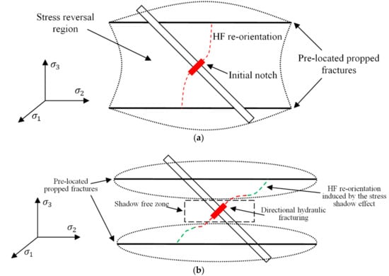
Figure 1.
Approaches to creating PHFs []: (a) Stress shadows of pre-located fractures overlap and create a stress reversal region between them. The PHF initiates from the oriented initial notch and propagates parallel to the in-situ σ3 orientation; (b) Stress shadows of pre-located fractures do not overlap and leave a stress shadow free zone between them. Directional hydraulic fracturing is applied to control the PHF initiation direction, and the stress shadow effect is used to induce the secondary PHF re-orientation.
The stress shadow effect modifies the local stress state in the orebody rock mass and is used in combination with the directional hydraulic fracturing method discussed in Huang et al. [] to control the HF initiation and propagation directions. Further details of the two proposed approaches can be found in He et al. [].
While the proposed approaches were proven feasible theoretically with numerical modelling [], no proof of these concepts has been given in the field. The field trial is a direct way to prove newly developed theoretical concepts. However, field tests can be expensive and time-consuming. Field scale numerical modelling could be an alternative [,], but numerical models’ ability to simulate field scale PHF re-orientation is uncertain since currently no field scale HF re-orientation trajectories are available as benchmarks for model validation.
Laboratory scale physical simulation experiments (i.e., controlled environment) combined with scaling laws can be used to simulate field scale HF propagation as elegantly demonstrated in various laboratory experiments by Bunger et al. []. In this paper, validated laboratory scale numerical modelling results on PHFs are transformed with dimensional analysis to predict PHF behaviour in field conditions as proof of the plausible practical feasibility of the concepts developed in lieu of field trials.
2. Previous Studies on Scaling Laws in Hydraulic Fracturing
The following presents the two scaling laws, namely non-dimensionalization (ND) and dimensional analysis, often used in previous studies and how they apply to hydraulic fracturing.
2.1. Nondimensionalization Concept Applied to Hydraulic Fracturing
Earlier studies developed governing equations to describe the propagation of HFs (Table 1 and Table 2). In most cases, these governing equations are unsolvable (i.e., have no analytical solutions). ND, which is also called scaling in some literature [], is used to determine the correlation between factors and to derive a particular solution to a problem []. Solutions derived by ND are in the form of factor groups.

Table 1.
Applications of nondimensionalization to deriving analytical or numerical solutions to axial planar HFs.
Table 2.
Applications of nondimensionalization to deriving analytical or numerical solutions to transverse radial HFs.
2.2. Dimensional Analysis Applied to Hydraulic Fracturing
Dimensional analysis [] is an alternative choice for HFs having irregular geometries, such as those undergo re-orientation. Bunger et al. [] used dimensionless relations to scale field scale hydraulic fracturing parameters to laboratory scale in their laboratory HF experiments. Later, Bunger et al. [] applied dimensional analysis to relate HF re-orientation trajectories in different scenarios considering the propagation of two closely located HFs.
From the aspect of scaling laws, HFs in different geotechnical scenarios reach the same values of dimensionless dependent factors (i.e., dimensionless fluid pressure, width and length) if the values of their dimensionless independent factor groups are identical [,]. Most factors involved in hydraulic fracturing theoretical studies are inherently dimensional, such as fluid pressure and the HF width. These factors are transformed into dimensionless forms in HF scaling by combining with other dimensional factors, resulting in factor groups that are dimensionless. The transformed dimensionless factor groups are termed dimensionless net pressure, dimensionless HF width, etc. accordingly, based on the physical meaning of the factor transformed in HF scaling [,,].
However, none of the scaling laws developed in previous studies are applicable to PHFs. Table 3 lists the dependent factors and independent factors considered in these studies. ND applications to regular shaped HFs attempt to relate the applied fluid pressure and HF dimensions to the influencing factors. For PHFs that focus on fracture re-orientation trajectories [], the established dimensionless relation is unable to project the PHF propagation path.
Table 3.
Dependent factors and independent factors considered in conventional hydraulic fracturing and HFs under the influence of the stress shadow effect.
Important dependent and independent factors involved in prescribed hydraulic fracturing are listed in Table 4 and differ from those in Table 3. Thus, previous dimensionless relation established by others does not apply to PHFs. The scaling laws for projecting PHFs laboratory scale numerical modelling results to field scale performance need to be developed.
Table 4.
Important factors governing prescribed hydraulic fractures.
3. Strategies for Relating Laboratory Scale Modelling of Prescribed Hydraulic Fractures to Field Scale
The scaling law established to relate Laboratory Scale PHFs to field scales is given in Section 3.1. The strategies for using this scaling law to study field scale PHFs are presented in Section 3.2. Further details can be found in He, Suorineni [].
3.1. Prescribed Hydraulic Fractures Dimensional Analysis
He et al. [] simulated prescribed hydraulic fracturing and studied the effects of various factors on their trajectories with the assumption that the PHF borehole lies on the σ2 − σ3 plane (Figure 2). In Figure 2, four dependent factors are used to quantify PHF re-orientation distances, including the vertical (Lvu) and horizontal (Lhu) propagation lengths of the PHF upper strand and the vertical (Lvl) and horizontal (Lhl) propagation lengths of the PHF lower strand. These factors measure how the PHF re-orientates from its preferred propagation direction and determine the PHF effectiveness in generating an additional joint set.
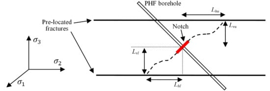
Figure 2.
Dependent factors considered in prescribed hydraulic fracturing []: the four factors Lvu, Lhu, Lvl, and Lhl quantify and measure the PHF trajectory.
He et al. [] concluded that PHFs in cases with the same differential stress magnitudes reach similar propagation distances. He et al. [] found that the differential stress σ1 − σ3 has a limited impact on PHF propagation if the PHF borehole is placed on the σ2 − σ3 plane. Evidence of this finding is given in Figure 3.
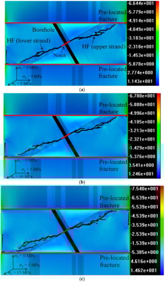
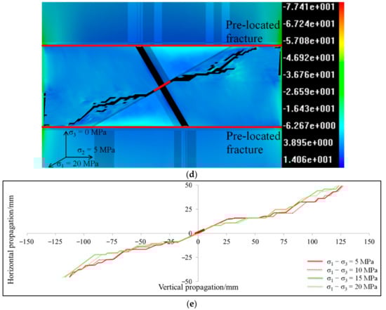
Figure 3.
Effect of the differential stress σ1 − σ3 on PHF propagation when the PHF borehole lies on the σ2 − σ3 plane []. In the modelling scenarios in (a–d), the in-situ σ1 and σ2 magnitudes are consistent with the in-situ σ3 magnitude increased from 5 MPa to 20 MPa with an interval of 5 MPa (the legends in (a–d) show the σ3 distributions): (a) Simulated PHF trajectory with a σ1 − σ3 magnitude of 5 MPa; (b) Simulated PHF trajectory with a σ1 − σ3 magnitude of 10 MPa; (c) Simulated PHF trajectory with a σ1 − σ3 magnitude of 15 MPa; (d) Simulated PHF trajectory with a σ1 − σ3 magnitude of 20 MPa; (e) Superimposed PHF trajectories from modelling results in (a–d). The superimposition shows the change of the differential stress σ1 – σ3 magnitude has limited influence on PHF propagation.
Using dimensional analysis, He et al. [] determined the correlation between factors involved in creating PHFs and established the dimensionless relation governing PHF propagation (Equation (1)). The dimensionless relation in Equation (1) was verified by He et al. [] through extensive numerical simulations:
The factor groups represented by each dimensionless factor in Equation (1) are given in Table 5. The definitions of both the dimensional factors in Table 5 and the dimensionless factors in Equation (1) are provided in the list of symbols in the paper.
Table 5.
Dimensionless relation between factors in prescribed hydraulic fracturing [].
3.2. The Strategies
Theoretically, modelled PHFs with different input parameters in Table 6, Table 7 and Table 8 result in similar dimensionless propagation paths (i.e., how the PHF propagates relative to the pre-located fractures) if the PHFs have the same values of dimensionless independent parameters (Table 9) as shown in Figure 4 and Figure 5. Note that PHF propagation paths in Figure 4 and Figure 5 are transformed in dimensionless forms, following Bunger et al.’s [] dimensional analysis of closely located HFs. For example, the PHFs in modelling Set 3 in Table 7 have different input parameters and propagate in numerical models with different sizes but reach similar dimensionless propagation paths (see Figure 5b).
Table 6.
Modelling scenarios for studying the validity of Equation (1). The values of parameters related to the differential stress, the net pressure and rock properties in Cases 1-2 to 1-5 (Cases 2-2 to 2-5) are increased by 20%, 40%, 60% and 80 % respectively compared with that in Case 1-1 (Case 2-1) with the values of other input parameters remaining consistent. The (σ2 − σ3)/σn ratios of modeling Sets 1 and 2 are kept constant as 2.5 and 3 respectively. The σc magnitudes in Cases 1-4 and 1-5 (Cases 2-4 and 2-5) are highly increased to test the reliability of Equation (1) in extreme cases [].
Table 7.
Modelling scenarios for studying the validity of Equation (1). The values of parameters related to the pre-located size, the pre-located fracture spacing and the borehole diameter in Cases 3-2 to 3-4 (Cases 4-2 to 4-4) are expanded to 2 times, 5 times and 10 times of that in Case 3-1 (Case 4-1) respectively with the values of other input parameters remaining consistent. The hydraulic conductively (k) value in each modelling scenario is scaled to keep modelling scenarios in each modelling set having the same dimensionless rock permeability (K) value. The (σ2 − σ3)/σn ratios of modeling Sets 3 and 4 are kept constant as 2.5 and 3 respectively [].
Table 8.
Modelling scenarios for studying the validity of Equation (1). The values of parameters related to rock hydraulic conductivity and fluid viscosity are given with various values with other input parameters remaining consistent. The (σ2 − σ3)/σn ratios of modeling Sets 3 and 4 are kept constant as 2.5 and 3 respectively [].
Table 9.
Values of dimensionless independent factor groups (Equation (1)) in modelling Sets 1 to 6 [].
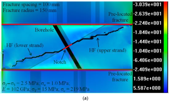
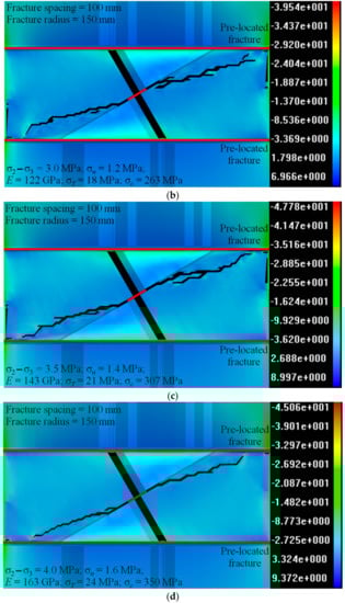
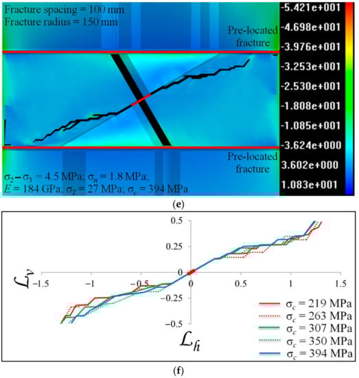
Figure 4.
Modelling results of Set 1 in Table 6 [] (the legends in (a–e) show the σ3 distributions): (a) Simulated PHF trajectory in Case 1-1 in Table 6; (b) Simulated PHF trajectory in Case 1-2 in Table 6; (c) Simulated PHF trajectory in Case 1-3 in Table 6; (d) Simulated PHF trajectory in Case 1-4 in Table 6; (e) Simulated PHF trajectory in Case 1-5 in Table 6; (f) Superimposed dimensionless PHF trajectories in modelling scenarios in Set 1 in Table 6. The superimposition shows these modelling scenarios have similar dimensionless PHF trajectories.
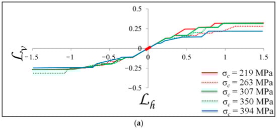
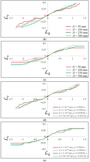
Figure 5.
Modelling results of Sets 2 to 6 in Table 6, Table 7 and Table 8 []. The superimposition in each figure in (a–e) indicates that the modelling scenarios in each modelling set have similar dimensionless PHF trajectories: (a) Superimposed dimensionless PHF trajectories in Set 2 in Table 6; (b) Superimposed dimensionless PHF trajectories in Set 3 in Table 7; (c) Superimposed dimensionless PHF trajectories in Set 4 in Table 7; (d) Superimposed dimensionless PHF trajectories in Set 5 in Table 8; (e) Superimposed dimensionless PHF trajectories in Set 6 in Table 8.
Herein, two terminologies used in the following contents are clarified. PHF dimensionless propagation path [] is the PHF re-orientation trajectory relative to the pre-located fractures (Figure 4f and Figure 5). PHF dimensionless length (i.e., vu, hu, vl or hl in Equation (1)) is the PHF re-orientation distance relative to the pre-located fracture spacing.
From Equation (1) and He et al.’s [] numerical modelling validation in Figure 4 and Figure 5, PHFs having the same dimensionless independent parameters lead to similar PHF dimensionless propagation path and PHF dimensionless length. Based on the above dimensional analysis principle, it is plausible to verify the concept of creating PHFs in field conditions based on laboratory scale numerical modelling in lieu of actual field trials.
The strategies for relating PHF propagation in different geotechnical scenarios by using the dimensionless relation established in Equation (1) are provided as follows. It is hypothesized that the evaluation of PHF propagation in field conditions is equivalent to predicting how the PHF propagates towards or away from the pre-located fractures and deriving the Lhu, Lvu, Lhl and Lvl values of the PHF (Figure 2) under sets of given input parameters from laboratory scale numerical modelling. Figure 6 gives the flow chart of the strategies, which include the following stages:
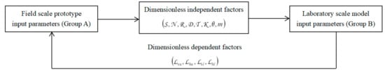
Figure 6.
Flow chart of the strategies for relating field scale PHFs to laboratory scale PHFs.
- Determining the values of the input parameters in the field scale prototype (i.e., Parameter Group A in Figure 6). The input parameters include objective and subjective ones. Objectives parameters relate to the geotechnical conditions, such as the differential stress, whereas the subjective parameters relate to parameters such as the pre-located fracture spacing and the PHF borehole dip angle. The values of the objective parameters dependent on the actual conditions at the mine site, and the values of the subjective parameters are determined by the field trial designed to test PHF feasibility.
- Calculating the values of the dimensionless independent factor groups (Equation (1)) in Parameter Group A. As evidenced by the validation results in Figure 4 and Figure 5, PHFs in two scenarios having the same values of dimensionless independent factor groups (Equation (1)) results in similar dimensionless propagation paths and lengths.
- Determining the values of the input parameters in the laboratory-scale numerical model (i.e., Parameter Group B in Figure 6). The numerical model has much smaller size (laboratory scale) than the field scale prototype and would also have scaled rock properties from the rock mass. The values of the dimensionless independent factor groups (Equation (1)) in the numerical model must be consistent with that in the field scale prototype. For example, if the differential stress magnitude in the numerical model is three times that in the field scale prototype, the rock UCS in the numerical model should accordingly increase by two times based on the form of the dimensionless differential stress (Table 5).
- Running the numerical model to simulate the laboratory scale PHF propagation. The PHF propagation path is transformed into the dimensionless form, such as that in Figure 4f and Figure 5, to evaluate the PHF re-orientation trajectory in the field scale []. The dimensionless PHF propagation length can also be deduced according to the forms of the dimensionless PHF length vu, hu, vl and hl (Table 5). Based on the validation results in Figure 4 and Figure 5, the field scale prototype has the same values of dimensionless PHF length as that in the laboratory-scale numerical model.
Calculating the PHF re-orientation lengths in the field scale prototype based on the values of the dimensionless PHF lengths and the forms of vu, hu, vl and hl (Table 5) (i.e., by multiplying the pre-located fracture spacing in the field scale).
4. Applicability of Prescribed Hydraulic Fracturing in Field Conditions Using Numerical Modelling and Dimensional Analysis
Following on from Section 3, the feasibility of creating PHFs in field conditions based on the principles of dimensionless analysis is evaluated in this section, using the geotechnical conditions in the E26 and E48 orebodies at Northparkes Mine (NPM). NPM is a property of China Molybdenum Corporation, located in New South Wales, Australia.
4.1. Geotechnical Conditions at Northparkes Mine
Northparkes Mine is the first block caving mine in Australia and the first to use hydraulic fracturing in the country. The orebody rock mass contains low grade copper and gold. Block caving was adopted to exploit the orebody as a profitable mining method []. The orebody was divided into mining blocks, namely the Endeavour 26 (E26) orebody and the Endeavour 48 (E48) orebody, the extraction levels of which are at depths of 450 m and 580 m respectively [,].
Both E26 and E48 orebodies consist of volcanics and monzonite porphyry with pipe-like geometry. In 1999, cave propagation in the E26 orebody stalled at a height of 95 meters as a result of arching at the cave back, creating an air gap between the muck top and the cave back. A lot of trials, including boundary weakening blasting and hydraulic fracturing, were carried out to re-activate caving. The final cost of caving inducement was around 1.1 million Australian Dollars []. Unfortunately, at about 2:50 p.m. on 24 November 1999, an air blast accident occurred during the mining operation, resulting in four fatalities [].
Hydraulic fracturing was used as a conventional orebody rock mass pre-conditioning method at Northparkes Mine []. HFs were created before undercutting to artificially weaken the rock mass quality rather than used to re-active caving once the stable arch forms. Field monitoring was performed to observe HF growth at the mine site, including stress change monitoring [], tilt monitoring [] and mine through mapping [].
The in-situ σ3 orientation at NPM is vertical, which leads to horizontal HFs by using the conventional hydraulic fracturing method. A stereo plot of natural fracture (NF) orientations derived from scan line mapping showed the orebody rock mass is dominated by sub-horizontal NFs []. Also, mine through mapping from both E26 orebody [] and E48 orebody [] indicated that HFs grew parallel to each other without dilating or extending the NFs. This implies the HFs were parallel to the NFs.
Based on the experience at NPM summarized above, it is concluded that the hydraulic fracturing was ineffective by not creating an additional joint set that could result in a blocky rock mass to enhance caving. Hence prescribed hydraulic fracturing would have been required to produce HFs that are not parallel to the existing NFs to result in a blocky rock mass.
The NPM experience provides a unique case for the hypothetical application of the use of PHFs. In this section, we employ numerical modelling on laboratory scales and use dimensional analysis to project the results to field scale as proof of the feasibility of the PHF concepts.
4.2. Numerical Modelling
First, the numerical modelling code used to simulate laboratory scale PHFs, the realistic failure process analysis (RFPA) 3D—flow code, is briefly introduced.
Hydraulic fracturing simulation has been widely studied previously [,,]. The RFPA3D—flow code is based on the basic realistic failure process analysis model [,] and the flow-stress-damage model []. Its mechanism was described in detail in Tang et al. [] and Li et al. [], and its two-dimensional version has a number of applications in simulating hydraulic fracturing in heterogeneous rock masses [,,].
RFPA is a poroelastic code and uses the classic Finite Element Method [,] to calculate the variables in both the solid mechanics and seepage flow fields. The consolidation theory [] is applied to describe the coupling process in which the elastic theory (Equations (2) to (4)) and Darcy’s law (Equation (5)) are used to govern the solid behaviour and fluid flow respectively:
where i, j = 1, 2, 3; σ is the stress, fi is the body force, ε is the strain, U is the displacement, σ′ is the effective stress, α is the Biot’s coefficient that determines the effect of pore pressure on the effective stress, p is pore pressure, δ is Kronecker’s constant, λ and G are the Lame parameters, εv is the volumetric strain, k is hydraulic conductivity, ∇2 is the Laplace operator and Q0 is Biot’s constant that measures the amount of water forced into the material under pressure with a constant volume.
Material homogeneity is considered and simulated by assigning different Young’s moduli and strength to elements according to the Weibull distribution []:
where P(u) is the probability density function for a given u value, m is the homogeneity index and uo is the mean value of the material property (i.e., Young’s modulus or rock UCS). The material is more homogeneous if a higher m value is assigned, and vice versa.
Each element is brittle-elastic with residual strength. An element is considered damaged when the element reaches its initial strength in either compression or tension. Damage mechanics [] is introduced to describe the element post-failure behaviour. Details of the damage constitutive laws in RFPA can be found in Tang [] and Tang et al. []. For a damaged element, it loses its Young’s modulus completely and becomes an ‘air element’ when it reaches its ultimate strain.
The RFPA3D—flow version is a static model. A flow rate boundary condition is applied to the nodes in the fluid injection area to simulate hydraulic fracturing, and the increment of the flow rate is kept low enough so that the HF can propagate steadily. The coupling process begins with calculating the variables in the seepage field (i.e., the flow rate and pore pressure). The effects of pore pressure on the rock material are in two aspects: its effect on the effective stress (Equation (4)) and the induced seepage force, which is a body force.
Finite element analysis is performed to calculate the stress and the displacement in the solid mechanics field. During the whole simulation process, the stiffness matrices for both the solid mechanics and seepage mechanics analyses are not immutable but vary with the damage or the failure of elements. To simulate hydraulic fracturing with RFPA, failed elements are used to represent the HF. The progressive failure of elements represents the HF propagation process.
RFPA’s ability to simulate hydraulic fracturing, especially HF re-orientation, was validated in two companion papers [,]. He et al. [] proved that RFPA is capable of simulating HF re-orientation from orientated perforations by comparing the simulation results with Abass et al.’s [] laboratory results. He et al. [] re-produced Bunger et al.’s [] experimental environments and concluded that RFPA is able to simulate the re-orientation of the HF due to the stress shadow effect.
4.2.1. Assumptions Used in Laboratory Scale Numerical Modelling
The rock properties and differential stress magnitudes in the E26 and E48 orebodies are provided in Table 10. The following assumptions are made in the numerical simulations:
Table 10.
Differential stress magnitudes and rock properties in the E26 and E48 orebodies at Northparkes Mine [,].
- The PHF borehole is assumed to lie on the σ2 − σ3 plane with a dip angle of 60°. This borehole dip angle is in a reasonable range because an acute dip angle (i.e., a sub-horizontal borehole) increases the required number of boreholes to precondition a given rock mass and a sharp dip angle (i.e., a sub-vertical borehole) restricts HF re-orientation induced by directional hydraulic fracturing.
- Rock tensile strength was not given in the literature and its ratio to rock UCS is assumed to be 0.1 [].
- The orebody rock type at NPM is monzonite porphyry. He et al. [] found that material homogeneity does not influence the feasibility of prescribed hydraulic fracturing (i.e., whether if the PHF succeeds in connecting the pre-located fractures) but has an impact on the PHF re-orientation trajectory. Liu et al. [] noted that the homogeneity index m [] value for a typical rock material is about 2. Herein, the m value of the orebody rock mass at NPM is assumed to be 5 to simulate a less homogeneous rock mass.
- Water is normally used as fracturing fluid in cave mining hydraulic fracturing, and its viscosity is about 0.001 Pa·s. In the numerical simulation, water is used to create PHFs between the pre-located fractures without proppants. More viscous fluid can be used to create the pre-located fractures with proppants to increase the pre-located fracture width (w) and hence enhance the stress shadow effect.
Table 11 provides a summary of the operation parameters at NPM used as field scale parameters for the PHF trials in lieu of actual field tests. The pre-located fracture spacing (H) and rock UCS (σc), which are the characteristic units [] used in He et al.’s [] dimensional analysis, in each numerical simulation are 100 mm and 120 MPa respectively. The values of other input parameters in each numerical simulation are scaled to keep the numerical model and the field scale prototype having the same values of dimensionless independent factor groups (Equation (1)). The field scale PHF trajectories are evaluated from the numerical simulation results, followed by the strategies described in Section 3.
Table 11.
Operation parameters designed for the expected PHF field trials in the E26 and E48 orebodies at Northparkes Mine.
4.2.2. Numerical Simulations Based on the E26 Orebody Condition
In Set 7, which is based on the E26 orebody characteristics (Table 11), the feasibility of prescribed hydraulic fracturing in the E26 orebody is studied. The differential stress between the in-situ σ2 and the in-situ σ3 in the E26 orebody is 3 MPa, which may favour HF re-orientation against its preferred direction. In Cases 7-1 to 7-3, the pre-located fractures have radii of 7.5 m with spacings of 5 m. The fracture radius is less than that in current cave mining hydraulic fracturing, which may reach 30 m. As discussed in He et al. [], the main function of the pre-located fracture in prescribed hydraulic fracturing is its influence on the local stress change, specifically, on the stress shadow.
In field applications, the induced stress shadow effect of the pre-located fracture might be weakened by the non-uniform distribution of the proppant; the potential screen out; and the interaction between the HF and the NF network []. These phenomena decrease the amount of proppant injected into the HF and weaken the induced stress shadow effect [,]. Hence three scenarios are studied in which the net pressure magnitude changes from 1 MPa to 2 MPa with an interval of 0.5 MPa to consider PHF propagation with different proppant efficiency. The net pressure magnitudes are in a reasonable range since the stress change monitoring performed by Mills et al. [] at Northparkes Mines showed the induced stress change observed 14 to 48 meters above a single HF was from 0.5 MPa to 1.4 MPa.
The evaluated PHF trajectories in Set 7 based on the simulated laboratory scale PHFs are provided in Figure 7. Note that He et al.’s [] numerical modelling results in Figure 4 and Figure 5 indicate that PHFs reach similar dimensionless propagation path (Section 3.2) if the PHFs have the same values of dimensionless independent parameters. The dimensionless propagation path reflects how the PHF propagates relative to (i.e., re-orientates towards or away) the pre-located fractures. Hence the simulated laboratory scale PHF trajectories are used to represent the predicted field scale PHF propagation relative to the pre-located fractures. Table 12 gives the evaluated field scale PHF lengths and the PHF dip angles. The PHF lengths are calculated by multiplying the field scale pre-located fracture spacing and the dimensionless PHF length derived from the laboratory numerical modelling results (see the definition of each dimensionless dependent factor in Table 5). The PHF dip angle is calculated by Equation (7) (in the case the PHF connects the pre-located fractures):
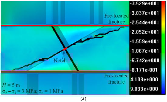
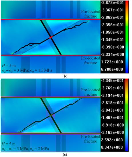
Figure 7.
Evaluated PHF trajectories in Set 7 in Table 11 (the legends in (a–c) show the σ3 distributions): (a) Evaluated PHF trajectory in Case 7-1; (b) Evaluated PHF trajectory in Case 7-2; (c) Evaluated PHF trajectory in Case 7-3.
Table 12.
Field scale PHF behaviors in Set 7 evaluated from laboratory scale numerical simulations.
Figure 7a–c show that the PHF in each case succeeds in connecting the pre-located fractures to form an oblique PHF. This implies creating PHFs that are not perpendicular to the far field σ3 orientation is feasible in field conditions. The variation of PHF dip angles in Table 12 indicate that the pre-located fracture induced net pressure magnitude has an impact on the PHF trajectory and the PHF tends to re-orientate more quickly towards the pre-located fractures with a higher net pressure magnitude. Therefore, the PHF dip angle could be controlled by the amount of proppants used during prescribed hydraulic fracturing. A higher pre-located fracture net pressure magnitude leads to a larger PHF dip angle as listed in Table 12.
The pre-located fracture net pressure magnitude in each scenario in Cases 7-1 to 7-3 is less than the differential stress magnitude (3 MPa), which means no stress reversal region occurs in the stress shadow around the pre-located fracture (the stress reversal region only occurs when the fracture induced stress is higher than the differential stress []). In spite of this, the PHF tends to propagate along the oriented notch orientation for a long distance in the stress shadow free zone as shown in the simulation results in Figure 7.
Abass et al. [] and Behrmann and Elbel [] drew the conclusion that HF re-orientation from oriented perforations was confined within two borehole diameters based on their experimental observation. He et al. [] argued that this statement might be debatable since HF could achieve a longer re-orientation distance in a low differential stress state, such as that in the stress shadow free zone between the pre-located fractures. The results in Figure 7 support He et al.’s [] opinion and indicate that the oriented initial notch is effective in prescribing the HF propagation path if the local stress state in the rock mass is modified by the stress shadow effect.
4.2.3. Numerical Simulations Based on the E48 Orebody Condition
Sets 8 and 9 (Table 11) are based on the geotechnical condition in the E48 orebody that has a higher differential stress magnitude and a weaker rock quality compared with that in the E26 orebody. According to Equation (8), the induced net pressure magnitude for a given pre-located fracture decreases in the rock mass with a lower E/(1 − ν2) ratio [].
where σn is the pre-located fracture net pressure, w is the pre-located fracture maximum width, E is rock Young’s modulus, ν is the Poisson’s ratio of the rock and r is the pre-located fracture radius.
The propped fracture widths in Cases 8-1 to 8-3 are assumed to be consistent with those in Cases 7-1 to 7-3 respectively, and the induced net pressure magnitude changes from 0.9 MPa to 1.7 MPa with an interval of 0.4 MPa based on Equation (8). The pre-located fracture radius and spacing in Set 8 are the same as that in Set 7.
The evaluated PHF trajectories in Set 8 are presented in Figure 8. The dimensional and dimensionless PHF length in these scenarios can be found in Table 13. In each scenario in Set 8, the HF fails to connect the pre-located fractures and propagates horizontally after initiating from the initial notch as shown in Figure 8a–c. These results indicate that the high differential stress in the E48 orebody provides significant restriction to HF re-orientation from the oriented initial notch. The Lvu and Lvl values in Set 8 (Table 13) show that the HF tends to have a longer re-orientation distance if a higher net pressure is induced. This means the pre-located fractures are capable of decreasing the local differential stress magnitude in the stress shadow free zone when the stress shadows overlap and hence enhancing HF re-orientation.
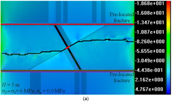
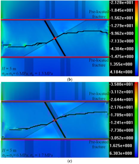
Figure 8.
Evaluated PHF trajectories in Set 8 in Table 11 (the legends in (a–c) show the σ3 distributions): (a) Evaluated PHF trajectory in Case 8-1; (b) Evaluated PHF trajectory in Case 8-2; (c) Evaluated PHF trajectory in Case 8-3.
Table 13.
Field scale PHF behaviors in Set 8 evaluated from laboratory scale numerical simulations.
In field applications, more viscous fracturing fluid can be used with or without a higher injection flow rate to increase the pre-located fracture initial width []. Also, a shorter fracture spacing can further decrease the local differential stress magnitude in the stress shadow free zone if stress shadows overlap [] and may favour PHF re-orientation.
In Set 9, higher net pressure magnitudes and shorter fracture spacings are assumed to examine the feasibility of prescribed hydraulic fracturing in a high differential stress condition.
The σn magnitude in Cases 9-1 and 9-3 is increased to 2.5 MPa, and the σn magnitude in Cases 3-2 and 3-4 is further increased to 3 MPa (Table 11). The fracture spacing in Cases 9-1 and 9-2 is decreased to 4 m from 5 m, and the fracture spacing in Cases 9-3 and 9-4 is further decreased to 3.5 from 5 m (Table 11). The evaluated PHF trajectories in Set 9 are provided in Figure 9.
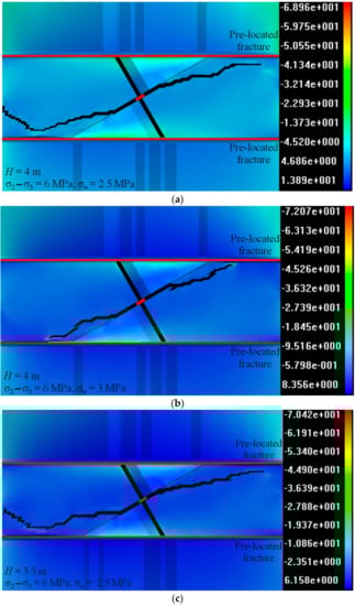
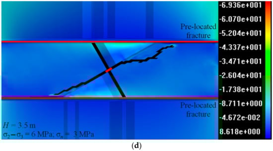
Figure 9.
Evaluated PHF trajectories in Set 9 in Table 11 (the legends in (a–d) show the σ3 distributions): (a) Evaluated PHF trajectory in Case 9-1; (b) Evaluated PHF trajectory in Case 9-2; (c) Evaluated PHF trajectory in Case 9-3; (d) Evaluated PHF trajectory in Case 9-4.
The dimensionless PHF length and the PHF dip angles in Set 9 are given in Table 14.
Table 14.
Field scale PHF behaviors in Set 9 evaluated from laboratory scale numerical simulations.
The results of Cases 9-1 (Figure 9a) and 9-3 (Figure 9c) are interesting because the HF shows a tendency to propagate away from the pre-located fracture after re-orientating towards it from the initial notch. This implies if the stress shadow effect is not strong enough to create a stress reversal region around the pre-located fracture or to partly change the local σ3 orientation in the stress shadow so that the propagating HF could be attracted (as that in Figure 1b), the PHF may finally propagate away from the pre-located fractures rather than parallel to them. In this situation that weak stress shadows are induced, a shorter fracture spacing is not helpful in enhancing the secondary HF re-orientation induced by the stress shadows of the pre-located fractures. In addition, the HF re-orientation distance induced by directional hydraulic fracturing is also restricted as indicated by the vu values in Cases 9-1 and 9-3 (Table 14) and the dimensional PHF vertical length, which are 1.64 m in Case 9-1 (4 m × 0.41) and 1.37 m in Case 9-3 (3.5 m × 0.39).
In Cases 9-2 and 9-4, the σn magnitudes is further increased to 3 MPa with the fracture spacings being 4 m and 3.5 m respectively. As shown in Figure 9b,d, the HF in each scenario has its tip finally connecting the pre-located fractures. This indicates the feasibility of prescribed hydraulic fracturing is very sensitive to the σn magnitude change. If the induced stress shadow effect is strong enough to induce the required HF re-orientation (i.e., attract the PHF to propagate towards rather than away from the pre-located fractures), a shorter fracture spacing enables the PHF to propagate more quickly towards the pre-located fractures as indicated by the PHF horizontal length in Table 14, which are 4.52 m (4 m × 1.13) and 4.60 m (4 m × 1.15) for the upper and lower strands respectively in Case 9-2 and 4.10 m (3.5 m × 1.17) and 3.36 m (3.5 m × 0.96) for the upper and lower strands respectively in Case 9-4.
5. Conclusions
Prescribed hydraulic fracturing was proposed in a previous study as a supplementary to the existing hydraulic fracturing strategy []. PHFs that are not perpendicular to the in-situ σ3 orientation aim to achieve a blocky orebody rock mass by generating an additional joint sets in the geotechnical conditions described by He et al. []. In this paper, the applicability of creating PHFs in field conditions is studied by using dimensional analysis. The following conclusions are made for the potential application of PHFs at caving mine sites.
- The appropriate borehole orientation is critical to the successful application of PHFs. The PHF borehole is strongly recommended to place on the σ2 − σ3 in order to overcome the restriction of the differential stress σ1 − σ3 on PHF re-orientation (Figure 3).
- Creating field scale PHFs is possible, and its feasibility is very sensitive to both the pre-located fracture net pressure magnitude and the in-situ differential stress magnitude. The pre-located fracture spacing and its ratio to the pre-located fracture radius also have an impact on the PHF trajectory.
- In a low differential stress state, such as that in the E26 orebody at Northparkes Mine (σ2 − σ3 = 3 MPa), water can be used as the fracturing fluid to create the pre-located fractures. The local differential stress magnitude in the stress shadow free zone (if the stress shadows overlap and hence have influence on the local stress state in the stress shadow free zone) is decreased significantly due to the stress shadow effect, which favours the use of directional hydraulic fracturing to control the PHF propagation path (Figure 7). The PHF tends to have a larger dip angle with the increase of the net pressure induced by the pre-located fractures.
- In a high differential stress state, such as that in the E48 orebody at Northparkes Mine (σ2 − σ3 = 6 MPa), more viscous fluid must be used to increase the pre-located fracture initial width in order to enhance the induced stress shadow effect. The PHF behaviour in the high differential stress condition is classified into three types, depending on the relative pre-located fracture net pressure (σn) magnitude to the differential stress (σ2 − σ3) magnitude.
- ○
- ○
- If the net pressure is increased slightly but still not high enough to induce the secondary PHF re-orientation (Figure 1b), such as that in Cases 9-1 and 9-3 in Table 11, the HF may tend to propagate away from the pre-located fractures and its re-orientation induced by directional hydraulic fracturing practice is also restricted as indicated by the simulation results in Figure 9a,c and the PHF propagation lengths listed in Table 14. In this situation, a shorter fracture spacing does not favour creating PHFs but results in HF re-orientation away from the pre-located fractures. Hence the spacing of the pre-located fractures should be carefully determined based on the σn/(σ2 − σ3) ratio. A shorter fracture spacing does not necessarily lead to enhanced PHF re-orientation towards the pre-located fractures.
- ○
- If the net pressure is high enough to induce the secondary PHF re-orientation, such as that in Cases 9-2 and 9-4 in Table 11, a PHF can be created and a shorter fracture spacing enables the PHF propagates more quickly towards the pre-located fractures with a larger dip angle.
Author Contributions
Q.H. initiated this research and wrote this manuscript. J.X. provided recommendations on technical issues. J.O. and C.Z. reviewed and improved this manuscript.
Funding
The work of this paper is supported by “the Fundamental Research Funds for the Central Universities” (grant number: 2018QNA31).
Acknowledgments
The first author would like to thank the China Scholarship Council (CSC) and the University of New South Wales (UNSW) for their support through the CSC scholarship and the UNSW Postdoctoral Writing Fellow scholarship respectively.
Conflicts of Interest
The authors declare no conflict of interest.
Abbreviations
| σ | stress, MPa |
| σ′ | effective stress, MPa |
| σ1 | maximum principal stress, MPa |
| σ2 | intermediate principal stress, MPa |
| σ3 | minimum principal stress, MPa |
| σn | pre-located fracture induced net pressure, MPa |
| σc | rock UCS, MPa |
| σT | rock tensile strength, MPa |
| ɛ | strain |
| ɛv | volumetric strain |
| α | Biot’s coefficient |
| δ | Kronecker’s constant |
| λ, G | Lame parameters |
| θBD | borehole dip angle |
| θBS | borehole strike angle |
| θPHF | PHF dip angle |
| D | borehole diameter, m |
| dimensionless borehole diameter | |
| E | Young’s modulus, MPa |
| f | body force, MPa |
| g | gravitational acceleration, m/s2 |
| H | pre-located fracture spacing, m |
| l | hydraulic fracture half-length, m |
| Lhu | horizontal length of the PHF upper strand, m |
| Lvu | vertical length of the PHF upper strand, m |
| Lhl | horizontal length of the PHF lower strand, m |
| Lvl | vertical length of the PHF lower strand, m |
| hu | dimensionless PHF upper strand horizontal length |
| vu | dimensionless PHF upper strand vertical length |
| hl | dimensionless PHF lower strand horizontal length |
| vl | dimensionless PHF lower strand vertical length |
| m | homogeneity index |
| dimensionless net pressure | |
| k | hydraulic conductivity, m/s |
| KIc | rock toughness, Pa·m1/2 |
| dimensionless rock permeability | |
| ρ | fluid density, kg/m3 |
| p | pore pressure, MPa |
| Q | the flow rate, m3/s |
| Qo | Biot’s constant |
| r | pre-located fracture radius, m |
| dimensionless pre-located fracture radius | |
| dimensionless differential stress | |
| t | injection time, s |
| dimensionless rock tensile strength | |
| μ | fluid viscosity, Pa·s |
| u | material property assigned to a given element |
| u0 | mean value of the material property |
| U | displacement, m |
| v | Poisson’s ratio |
| w | pre-located fracture maximum width, m |
References
- Montgomery, C.T.; Smith, M.B. Hydraulic fracturing: History of an enduring technology. J. Pet. Technol. 2010, 62, 26–40. [Google Scholar] [CrossRef]
- Warpinski, N.R. Hydraulic fracturing in tight, fissured media. J. Pet. Technol. 1991, 43, 146–209. [Google Scholar] [CrossRef]
- Rummel, F.; Kappelmeyer, O. The Falkenberg Geothermal Frac Project: Concepts and Experimental Results. In Hydraulic Fracturing and Geothermal Energy; Nijhoff: Hague, The Netherlands, 1983; pp. 59–74. [Google Scholar]
- He, Q.; Suorineni, F.; Oh, J. Review of Hydraulic Fracturing for Preconditioning in Cave Mining. Rock Mech. Rock Eng. 2016, 49, 4893–4910. [Google Scholar] [CrossRef]
- Garagash, D.I. Propagation of a plane-strain hydraulic fracture with a fluid lag: Early-time solution. Int. J. Solids Struct. 2006, 43, 5811–5835. [Google Scholar] [CrossRef]
- Carbonell, R.; Desroches, J.; Detournay, E. A comparison between a semi-analytical and a numerical solution of a two-dimensional hydraulic fracture. Int. J. Solids Struct. 1999, 36, 4869–4888. [Google Scholar] [CrossRef]
- Bunger, A.P.; Detournay, E.; Garagash, D.I. Toughness-dominated hydraulic fracture with leak-off. Int. J. Fract. 2005, 134, 175–190. [Google Scholar] [CrossRef]
- Nordgren, R. Propagation of a vertical hydraulic fracture. Soc. Pet. Eng. J. 1972, 12, 306–314. [Google Scholar] [CrossRef]
- Zhang, X.; Detournay, E.; Jeffrey, R. Propagation of a penny-shaped hydraulic fracture parallel to the free-surface of an elastic half-space. Int. J. Fract. 2002, 115, 125–158. [Google Scholar] [CrossRef]
- Abe, H.; Keer, L.; Mura, T. Growth rate of a penny—Shaped crack in hydraulic fracturing of rocks, 2. J. Geophys. Res. 1976, 81, 6292–6298. [Google Scholar] [CrossRef]
- Advani, S.; Torok, J.; Lee, J.; Choudhry, S. Explicit time-dependent solutions and numerical evaluations for penny—Shaped hydraulic fracture models. J. Geophys. Res. Solid Earth 1987, 92, 8049–8055. [Google Scholar] [CrossRef]
- Bunger, A.P.; Detournay, E. Early-time solution for a radial hydraulic fracture. J. Eng. Mech. 2007, 133, 534–540. [Google Scholar] [CrossRef]
- Savitski, A.; Detournay, E. Propagation of a penny-shaped fluid-driven fracture in an impermeable rock: Asymptotic solutions. Int. J. Solids Struct. 2002, 39, 6311–6337. [Google Scholar] [CrossRef]
- Hubbert, M.K.; Willis, D.G. Mechanics of Hydraulic Fracturing; Gulf Professional: Houston, TX, USA, 1972. [Google Scholar]
- Fisher, M.; Heinze, J.; Harris, C.; Davidson, B.; Wright, C.; Dunn, K. Optimizing horizontal completion techniques in the Barnett shale using microseismic fracture mapping. In Proceedings of the SPE Annual Technical Conference and Exhibition, Houston, TX, USA, 26–29 September 2004; Society of Petroleum Engineers: Richardson, TX, USA, 2004. [Google Scholar]
- Huang, B.-X.; Yu, B.; Feng, F.; Li, Z.; Wang, Y.-Z.; Liu, J.-R. Field investigation into directional hydraulic fracturing for hard roof in Tashan Coal Mine. J. Coal Sci. Eng. (China) 2013, 19, 153–159. [Google Scholar] [CrossRef]
- He, Q.; Suorineni, F.; Oh, J. Strategies for Creating Prescribed Hydraulic Fractures in Cave Mining. Rock Mech. Rock Eng. 2017, 50, 967–993. [Google Scholar] [CrossRef]
- Zhou, S.; Zhuang, X.; Zhu, H.; Rabczuk, T. Phase Field Modelling of Crack Propagation, Branching and Coalescence in Rocks. Theor. Appl. Fract. Mech. 2018, 96, 174–192. [Google Scholar] [CrossRef]
- Zhou, S.; Zhuang, X.; Rabczuk, T. A Phase-Field Modeling Approach of Fracture Propagation in Poroelastic Media. Eng. Geol. 2018, 240, 189–203. [Google Scholar] [CrossRef]
- Bunger, A.P.; Jeffrey, R.G.; Detournay, E. Application of scaling laws to laboratory-scale hydraulic fractures. In Proceedings of the 40th US Symposium on Rock Mechanics (USRMS), Anchorage, AK, USA, 25–29 June 2005; American Rock Mechanics Association: Alexandria, VA, USA, 2005. [Google Scholar]
- Schaeffer, D.G.; Cain, J.W. Nondimensionalization and Scaling, Ordinary Differential Equations: Basics and Beyond; Springer: Berlin, Germany, 2016; pp. 161–194. [Google Scholar]
- Holmes, M.H. Introduction to the Foundations of Applied Mathematics; Springer Science & Business Media: Berlin, Germany, 2009. [Google Scholar]
- Lecampion, B.; Detournay, E. An Implicit Algorithm for the Propagation of a Hydraulic Fracture with a Fluid Lag. Comput. Methods Appl. Mech. Eng. 2007, 196, 4863–4880. [Google Scholar] [CrossRef]
- Garagash, D. Hydraulic Fracture Propagation in Elastic Rock with Large Toughness. In Proceedings of the 4th North American Rock Mechanics Symposium, Seattle, WA, USA, 31 July–3 August 2000; pp. 221–228. [Google Scholar]
- Adachi, J.I.; Detournay, E. Plane Strain Propagation of a Hydraulic Fracture in a Permeable Rock. Eng. Fract. Mech. 2008, 75, 4666–4694. [Google Scholar] [CrossRef]
- Adachi, J.I.; Detournay, E. Self-Similar Solution of A Plane-Strain Fracture Driven by A Power-Law Fluid. Int. J. Numer. Anal. Methods Geomech. 2002, 26, 579–604. [Google Scholar] [CrossRef]
- Garagash, D.I.; Detournay, E. Plane-Strain Propagation of a Fluid-Driven Fracture: Small Toughness Solution. J. Appl. Mech. 2005, 72, 916–928. [Google Scholar] [CrossRef]
- Barenblatt, G.I. Scaling, Self-Similarity, and Intermediate Asymptotics: Dimensional Analysis and Intermediate Asymptotics; Cambridge University Press: Cambridge, UK, 1996. [Google Scholar]
- Bunger, A.; Jeffrey, R.; Kear, J.; Zhang, X.; Morgan, M. Experimental investigation of the interaction among closely spaced hydraulic fractures. In Proceedings of the 45th US Rock Mechanics/Geomechanics Symposium, San Francisco, CA, USA, 26–29 June 2011; American Rock Mechanics Association: Alexandria, VA, USA, 2011. [Google Scholar]
- Bunger, A.P.; Zhang, X.; Jeffrey, R.G. Parameters affecting the interaction among closely spaced hydraulic fractures. SPE J. 2012, 17, 292–306. [Google Scholar] [CrossRef]
- Pater, C.J.D.; Weijers, L.; Cleary, M.P.; Quinn, T.S.; Barr, D.T.; Johnson, D.E. Experimental Verification of Dimensional Analysis for Hydraulic Fracturing. SPE Prod. Facil. 1994, 9, 230–238. [Google Scholar] [CrossRef]
- He, Q.; Suorineni, F.; Ma, T.; Oh, J. Parametric Study and Dimensional Analysis on Prescribed Hydraulic Fractures in Cave Mining. Tunn. Undergr. Space Technol. 2018, 78, 47–63. [Google Scholar] [CrossRef]
- Van As, A.; Jeffrey, R.; Chacon, E.; Barrera, V. Preconditioning by hydraulic fracturing for block caving in a moderately stressed naturally fractured orebody. In Proceedings of the MassMin, Santiago, Chile, 22–25 August 2004; pp. 535–541. [Google Scholar]
- Jeffrey, R.G.; Bunger, A.; Lecampion, B.; Zhang, X.; Chen, Z.; van As, A.; Allison, D.P.; De Beer, W.; Dudley, J.W.; Siebrits, E. Measuring hydraulic fracture growth in naturally fractured rock. In Proceedings of the SPE annual technical conference and exhibition, New Orleans, LA, USA, 4–7 October 2009; Society of Petroleum Engineers: Richardson, TX, USA, 2009. [Google Scholar]
- Van As, A.; Jeffrey, R. Caving induced by hydraulic fracturing at Northparkes mines. In Proceedings of the 4th North American Rock Mechanics Symposium, Seattle, WA, USA, 31 July–3 August 2000; American Rock Mechanics Association: Alexandria, VA, USA, 2000. [Google Scholar]
- Van As, A.; Jeffrey, R. Hydraulic Fracturing as a Cave Inducement Technique at Northparkes Mines; Australasian Institute of Mining and Metallurgy: Carlton, Australia, 2000. [Google Scholar]
- Fowler, J.; Hebblewhite, B.; Sharma, P. Managing the hazard of wind blast/air blast in caving operations in underground mines. In Proceedings of the 10th ISRM Congress, Sandton, South Africa, 8–12 September 2003; International Society for Rock Mechanics: Lisboa, Portugal, 2003. [Google Scholar]
- Van As, A.; Jeffrey, R. Hydraulic fracture growth in naturally fractured rock: Mine through mapping and analysis. In Proceedings of the 5th North American Rock Mechanics Symposium and the 17th Tunnelling Association of Canada Conference, Toronto, ON, Canada, 7–10 July 2002. [Google Scholar]
- Mills, K.; Jeffrey, R.; Karzulovic, A.; Alfaro, M. Remote high resolution stress change monitoring for hydraulic fractures. In Proceedings of the Proud to be miners, MassMin, Santiago, Chile, 22–25 August 2004. [Google Scholar]
- Chen, Z.; Jeffrey, R. Tilt monitoring of hydraulic fracture preconditioning treatments. In Proceedings of the 43rd US Rock Mechanics Symposium & 4th US-Canada Rock Mechanics Symposium, Asheville, NC, USA, 28 June–1 July 2009; American Rock Mechanics Association: Alexandria, VA, USA, 2009. [Google Scholar]
- Rabczuk, T.; Gracie, R.; Song, J.-H.; Belytschko, T. Immersed Particle Method for Fluid–Structure Interaction. Int. J. Numer. Methods Eng. 2010, 81, 48–71. [Google Scholar]
- Zhuang, X.; Huang, R.; Liang, C.; Rabczuk, T. A Coupled Thermo-Hydro-Mechanical Model of Jointed Hard Rock for Compressed Air Energy Storage. Math. Probl. Eng. 2014, 2014, 179169. [Google Scholar] [CrossRef]
- Rabczuk, T.; Zi, G.; Natarajan, S.; Bordas, S. A Simple and Robust Three-Dimensional Cracking Particle Method without Enrichment. Comput. Methods Appl. Mech. Eng. 2010, 199, 2437–2455. [Google Scholar] [CrossRef]
- Tang, C. Numerical simulation of progressive rock failure and associated seismicity. Int. J. Rock Mech. Min. Sci. 1997, 34, 249–261. [Google Scholar] [CrossRef]
- Tang, C.; Yang, W.; Fu, Y.; Xu, X. A new approach to numerical method of modelling geological processes and rock engineering problems—Continuum to discontinuum and linearity to nonlinearity. Eng. Geol. 1998, 49, 207–214. [Google Scholar] [CrossRef]
- Tang, C.; Tham, L.; Lee, P.; Yang, T.; Li, L. Coupled analysis of flow, stress and damage (FSD) in rock failure. Int. J. Rock Mech. Min. Sci. 2002, 39, 477–489. [Google Scholar] [CrossRef]
- Li, L.; Tang, C.; Li, G.; Wang, S.; Liang, Z.; Zhang, Y. Numerical simulation of 3D hydraulic fracturing based on an improved flow-stress-damage model and a parallel FEM technique. Rock Mech. Rock Eng. 2012, 45, 801–818. [Google Scholar] [CrossRef]
- Wang, S.; Sloan, S.; Fityus, S.; Griffiths, D.; Tang, C. Numerical modeling of pore pressure influence on fracture evolution in brittle heterogeneous rocks. Rock Mech. Rock Eng. 2013, 46, 1165–1182. [Google Scholar] [CrossRef]
- Wang, S.; Sun, L.; Au, A.; Yang, T.; Tang, C. 2D-numerical analysis of hydraulic fracturing in heterogeneous geo-materials. Construct. Build. Mater. 2009, 23, 2196–2206. [Google Scholar] [CrossRef]
- Yang, T.; Tham, L.; Tang, C.; Liang, Z.; Tsui, Y. Influence of heterogeneity of mechanical properties on hydraulic fracturing in permeable rocks. Rock Mech. Rock Eng. 2004, 37, 251–275. [Google Scholar] [CrossRef]
- Logan, D.L. A First Course in the Finite Element Method; Cengage Learning: Boston, MA, USA, 2011. [Google Scholar]
- Fish, J.; Belytschko, T. A First Course in Finite Elements; John Wiley & Sons: Hoboken, NJ, USA, 2007. [Google Scholar]
- Biot, M.A. General theory of three-dimensional consolidation. J. Appl. Phys. 1941, 12, 155–164. [Google Scholar] [CrossRef]
- Weibull, W. A Statistical Distribution Function of Wide Applicability. J. Appl. Mech. 1951, 18, 293–297. [Google Scholar]
- Krajcinovic, D. Damage mechanics. Mech. Mater. 1989, 8, 117–197. [Google Scholar] [CrossRef]
- He, Q.; Suorineni, F.T.; Ma, T.; Oh, J. Effect of discontinuity stress shadows on hydraulic fracture re-orientation. Int. J. Rock Mech. Min. Sci. 2017, 91, 179–194. [Google Scholar] [CrossRef]
- He, Q.; Suorineni, F.; Oh, J.; Ma, T. Modeling directional hydraulic fractures in heterogeneous rock masses. In Proceedings of the MassMin, Sydney, Australia, 9–11 May 2016. [Google Scholar]
- Abass, H.H.; Brumley, J.L.; Venditto, J.J. Oriented perforations-a rock mechanics view, SPE annual technical conference and exhibition. In Proceedings of the SPE Annual Technical Conference and Exhibition, New Orleans, LA, USA, 25–28 September 1994; Society of Petroleum Engineers: Richardson, TX, USA, 1994. [Google Scholar]
- Barták, J.; Ordina, I.; Romancov, G.; Zlamal, J. Underground Space: The 4th Dimension of Metropolises; Taylor & Francis: Didcot, UK, 2007. [Google Scholar]
- Liu, H.; Roquete, M.; Kou, S.; Lindqvist, P.-A. Characterization of rock heterogeneity and numerical verification. Eng. Geol. 2004, 72, 89–119. [Google Scholar] [CrossRef]
- Smith, M.B.; Montgomery, C. Hydraulic Fracturing; CRC Press: Boca Raton, FL, USA, 2015. [Google Scholar]
- Roussel, N.P.; Manchanda, R.; Sharma, M.M. Implications of Fracturing Pressure Data Recorded during a Horizontal Completion on Stage Spacing Design. In Proceedings of the SPE Hydraulic Fracturing Technology Conference, The Woodlands, TX, USA, 6–8 February 2012. [Google Scholar]
- Manchanda, R.; Sharma, M.M. Impact of Completion Design on Fracture Complexity in Horizontal Wells. Spe Drill. Complet. 2014, 29, 78–87. [Google Scholar] [CrossRef]
- Behrmann, L.; Elbel, J. Effect of perforations on fracture initiation. J. Pet. Technol. 1991, 43, 608–615. [Google Scholar] [CrossRef]
- Tada, H.; Paris, P.; Irwin, G. The analysis of cracks handbook. ASME Press: New York, NY, USA, 2000; Volume 2, p. 1. [Google Scholar]
- Rafiee, M.; Soliman, M.Y.; Pirayesh, E.; Emami Meybodi, H. Geomechanical considerations in hydraulic fracturing designs. In Proceedings of the SPE Canadian Unconventional Resources Conference, Calgary, AB, Canada, 30 October–1 November 2012; Society of Petroleum Engineers: Richardson, TX, USA, 2012. [Google Scholar]
© 2018 by the authors. Licensee MDPI, Basel, Switzerland. This article is an open access article distributed under the terms and conditions of the Creative Commons Attribution (CC BY) license (http://creativecommons.org/licenses/by/4.0/).