Computational Fluid Dynamics Approach to Predict the Actual Wind Speed over Complex Terrain


Research Institute for Applied Mechanics (RIAM), Kyushu University, 6-1 Kasuga-kouen, Kasuga, Fukuoka 816-8580, Japan
Energies 2018, 11(7), 1694; https://doi.org/10.3390/en11071694
Submission received: 24 May 2018
/
Revised: 20 June 2018
/
Accepted: 22 June 2018
/
Published: 29 June 2018
(This article belongs to the Collection Wind Turbines)
Abstract
:This paper proposes a procedure for predicting the actual wind speed for flow over complex terrain with CFD. It converts a time-series of wind speed data acquired from field observations into a time-series data of actual scalar wind speed by using non-dimensional wind speed parameters, which are determined beforehand with the use of CFD output. The accuracy and reproducibility of the prediction procedure were investigated by simulating the flow with CFD with the use of high spatial resolution (5 m) surface elevation data for the Noma Wind Park in Kagoshima Prefecture, Japan. The errors of the predicted average monthly wind speeds relative to the observed values were less than approximately 20%.
1. Introduction
A significant reduction in CO2 emissions to prevent global warming is currently an urgent issue. For this reason, the effective use of clean, environmentally-friendly wind energy has received attention. Since the power output of a wind turbine (WT) is proportional to the cube of the wind speed, it is extremely important to accurately select sites with wind conditions that are well suited for WT deployment with a high degree of precision. In Japan, most terrain is complex and few areas are flat, which is quite different from the terrain in Europe and the U.S. Thus, it is very important to take into account the effects of terrain on the wind flow, such as flow impingement, flow separation, flow reattachment and reverse flow. Given this background, micro-siting software, which can simulate wind over the complex terrain that is unique to Japan, is currently being developed based on computational fluid dynamics (CFD). This development is being carried out with the vision that the software can also be applied for micro-siting of WTs over complex terrain in any other part of the world [1,2,3,4,5,6,7,8,9,10,11,12].
The author’s research group has also been developing such software, specifically an unsteady, nonlinear wind simulator called RIAM-COMPACT (Research Institute for Applied Mechanics, Kyushu University, COMputational Prediction of Airflow over Complex Terrain), which is applicable for almost any flat or complex terrain across the world [13,14,15,16,17,18,19,20,21,22]. RIAM-COMPACT is based on a large-eddy simulation (LES), which is a turbulence model, and simulates airflow in small domains of approximately a few hundreds of meters to a few kilometers. One of the major features of RIAM-COMPACT is that it can, with high accuracy, predict and visualize, in the form of animation, the effects of terrain on the wind flow such as flow separation, the formation of reverse flow regions, which results from flow separation, local flow acceleration and reattachment of separated shear layers.
At a planned construction site for a wind power facility, it is standard practice for an observation pole of 30 m or taller to be set up to collect time-series data of wind direction, speed and other meteorological variables over a period of one year. If these observation data can be loaded into a CFD model and both the observed data and the CFD output can be combined efficiently, economic assessments of the wind power facility, including assessments of the annual energy production and capacity factor at an arbitrary location within the facility, can be made with high accuracy.
Accordingly, the present study proposes a procedure to predict the actual wind speed over complex terrain based on time-series data collected from field observations and CFD output. In this procedure, a time-series of wind speed data acquired from field observations is converted into a time-series of the actual scalar wind speed for the prediction point with the use of (non-dimensional) wind speed parameters, which were determined beforehand with the use of CFD output. The validity of the proposed procedure is examined for Noma Wind Park, Kagoshima Prefecture, Japan, with the use of observation data collected with propeller vane anemometers mounted on the nacelles of WTs.
2. Overview of Noma Wind Park, Kagoshima Prefecture
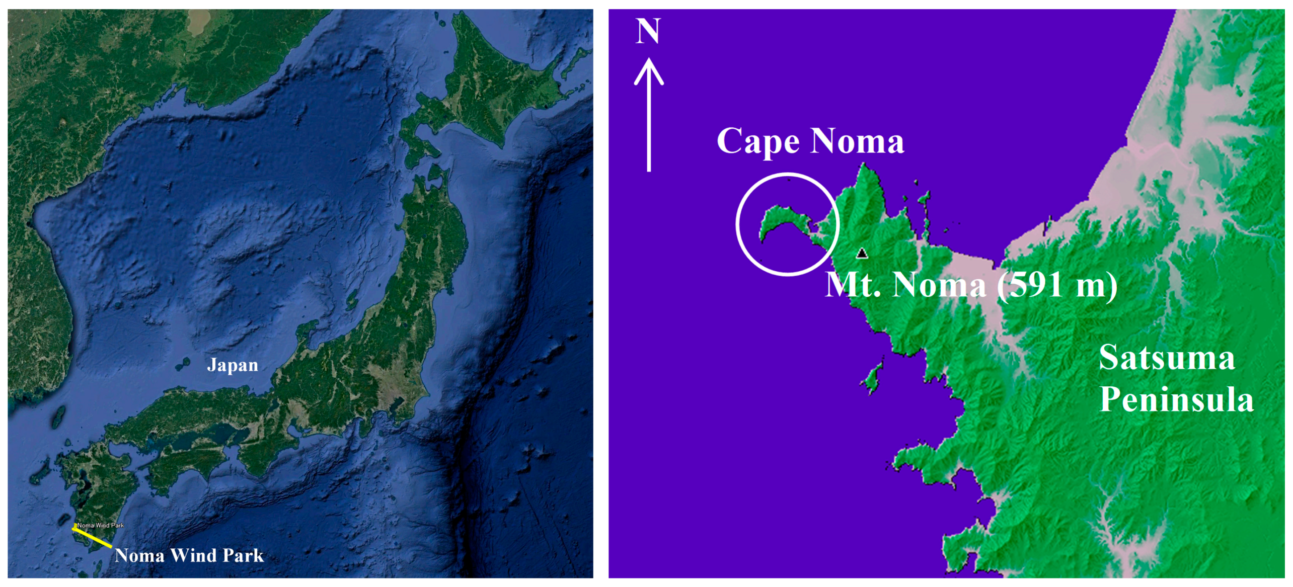
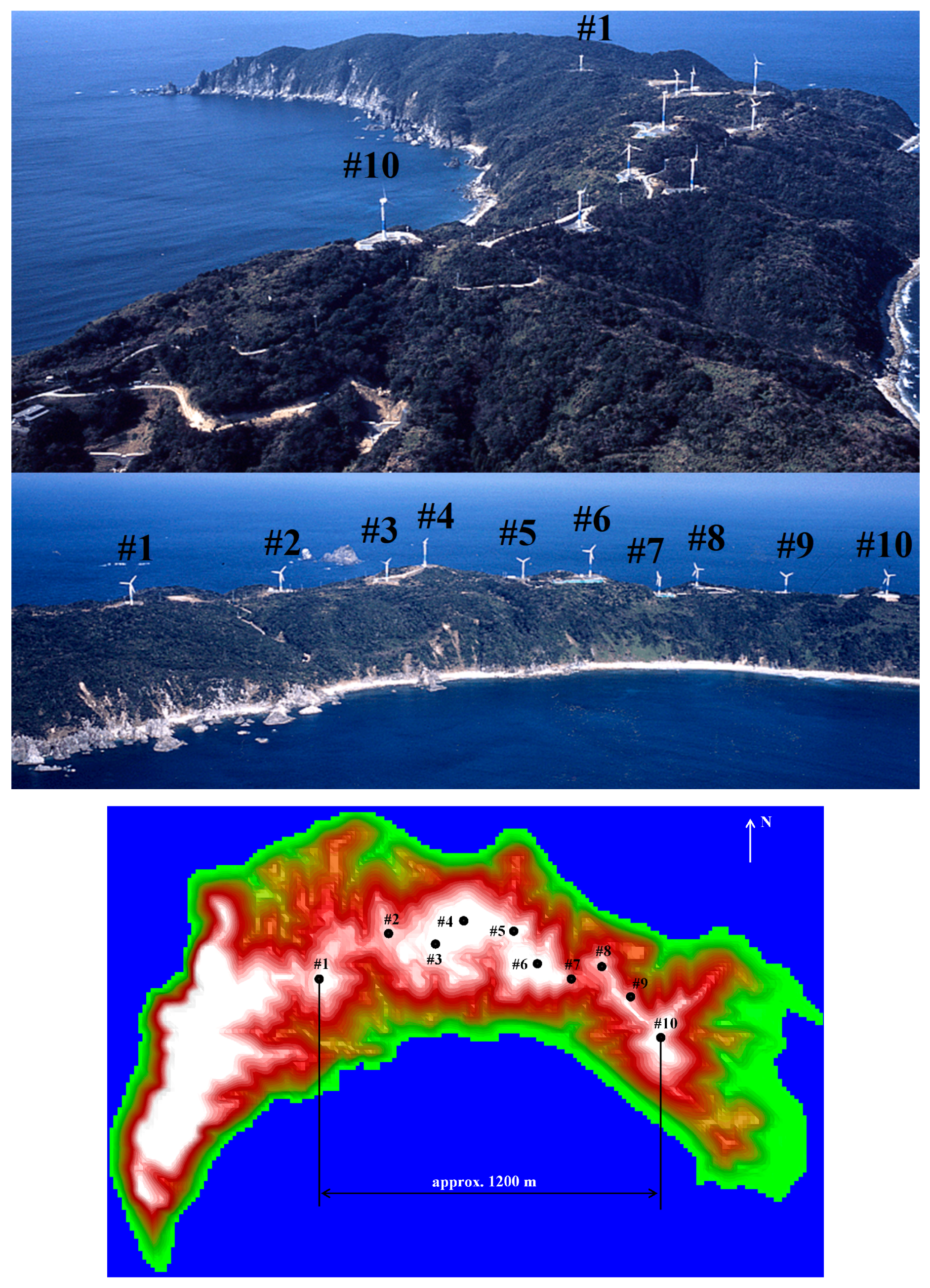
Noma Wind Park is in Minami Satsuma City in the southwestern part of Kagoshima Prefecture, Japan (marked by the circle in Figure 1). The terrain at and in the surrounding area of Noma Wind Park is steep complex terrain (Figure 2). While the wind park is surrounded by the ocean, a steep cliff with a slope angle of more than 30 degrees is at the western end of the cape. The maximum elevation of the terrain surface is 143 m. In Noma Wind Park, ten WTs that are owned by Kyushu Electric Power Co., Inc. (Fukuoka, Japan), have been deployed, and verification tests have been conducted. The rated output of each WT is 300 kW; thus, the total rated output from the ten WTs combined is 3000 kW. Table 1 and Table 2 give an overview of the WTs deployed in Noma Wind Park.
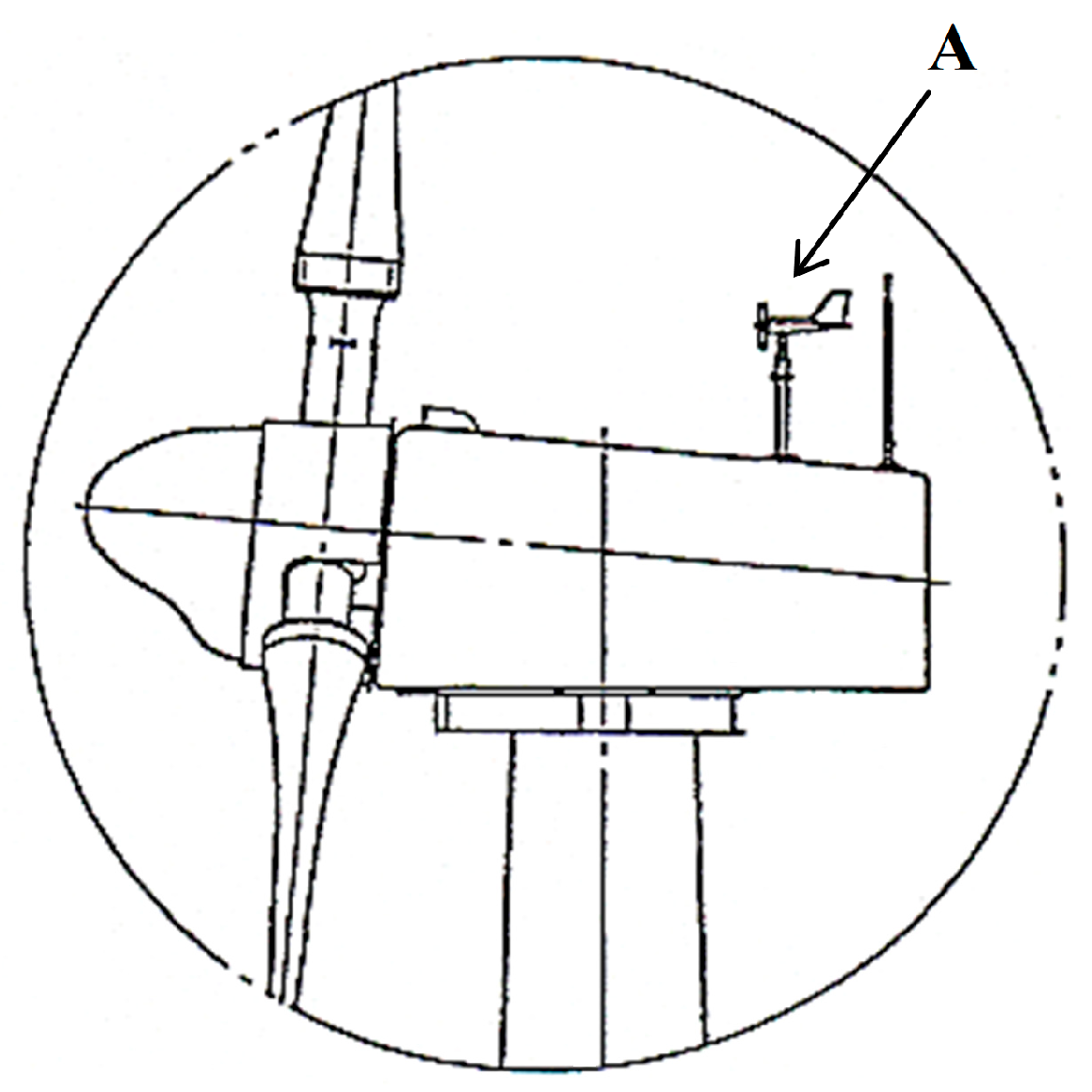
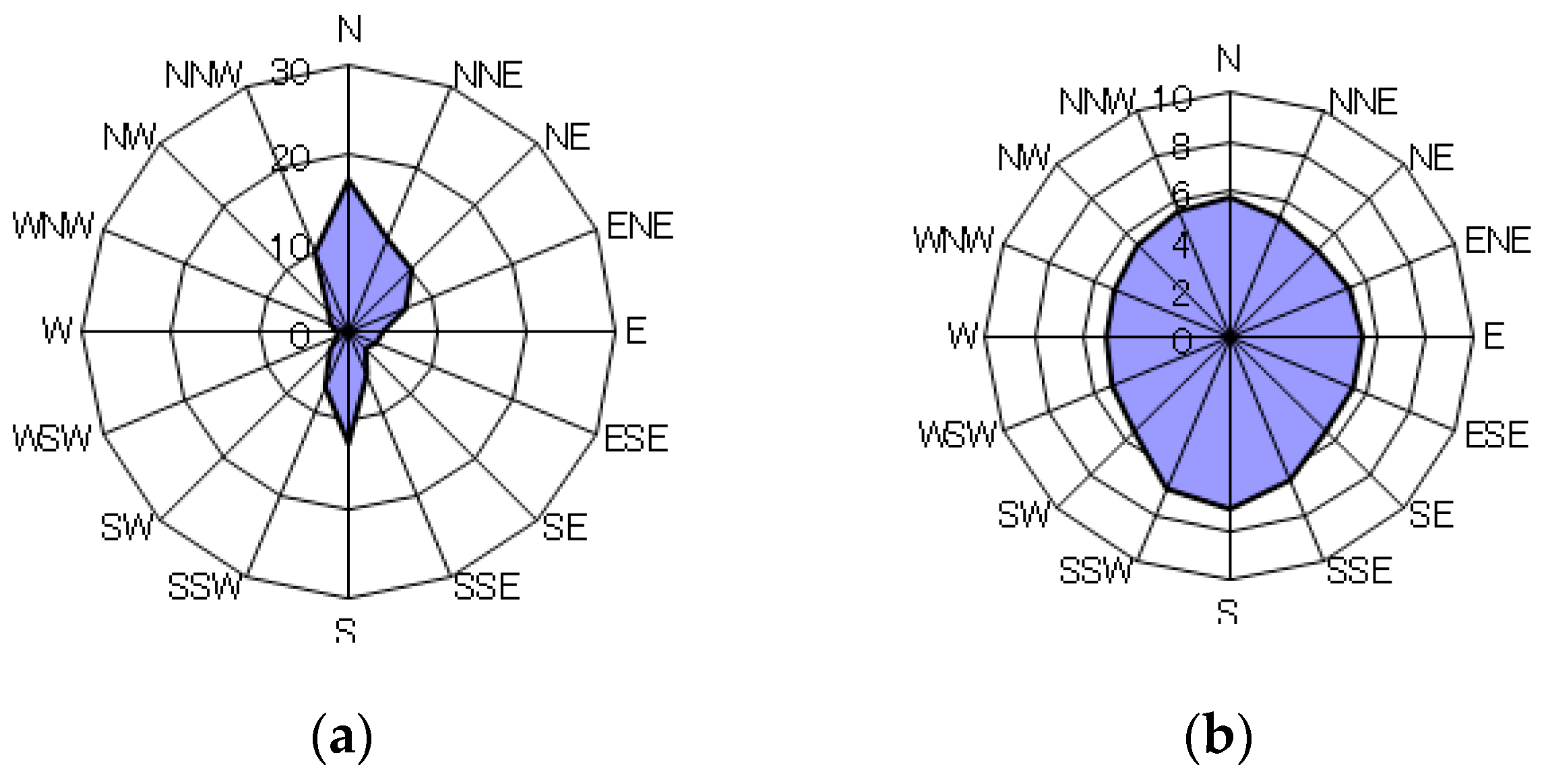
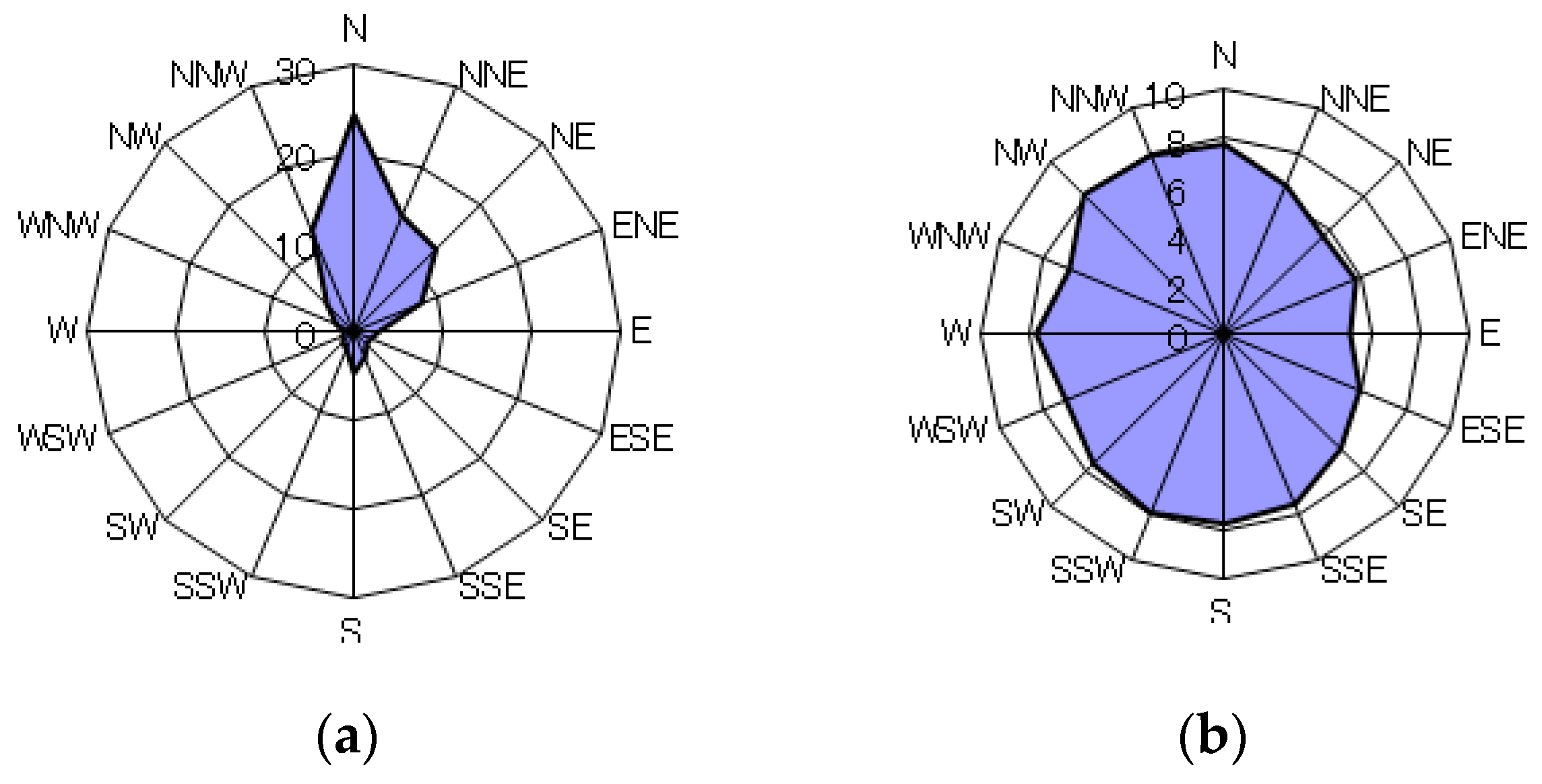
Propeller vane anemometers are mounted on all of the WTs deployed in Noma Wind Park (indicated by “A” in Figure 3). The present study employs time-series observation data from these propeller vane anemometers. The data were recorded every one minute. Details of the wind characteristics at Noma Wind Park from June 2002–May 2003 are summarized in Uchida. According to Uchida, the prevailing wind direction at this site is northerly, and the monthly average wind speed is large from November–March (see Figure 4 and Figure 5). The present study validates the proposed procedure for predicting the actual wind speed with the use of observation data from February 2003, the month during the observation period in which the least data are missing for all ten WTs and also in which the value of the monthly average wind speed is large. For February 2003, 40,047 and 273 data values are available for analysis and missing, respectively (percentage of non-missing data: 99%).
3. Numerical Simulation Technique and Set-up
The present study employs the wind farm design tool called RIAM-COMPACT. This software simulates neutral wind flow with the use of a collocated grid arrangement in a general curvilinear coordinate system. For the governing equations of the flow, a filtered continuity equation for incompressible fluid (Equation (1)) and filtered Navier–Stokes equations (Equation (2)) are used. The effects of the surface roughness have been taken into consideration by reconstructing surface irregularities at high resolution (horizontal spatial resolution: 5 m).
For the computational algorithm, a fractional step (FS) method [23] is used. A time marching method based on the Euler explicit method is adopted. Poisson’s equation for pressure is solved by a successive over-relaxation (SOR) method. For discrimination of all the spatial terms in the governing equations except for the convective term in Equation (2), a second-order central difference scheme is applied. For the convective term, a third-order upwind difference scheme is used. For the fourth-order central difference term that constitutes the discretized convective term, the interpolation technique of Kajishima [24], which is based on a four-point difference scheme and a four-point interpolation scheme, is used. For the weighting of the numerical diffusion term in the discretized convective term, α = 3.0 is commonly applied in the Kawamura–Kuwahara scheme [25]. However, α = 0.5 is used in the present study to minimize the influence of numerical diffusion. For the LES subgrid-scale modeling, the standard Smagorinsky model [26] (Equations (3)–(8)) is adopted with a model coefficient of 0.1 in conjunction with a wall-damping function.
4. Procedure for Predicting Actual Wind Speed
The procedure for predicting the actual scalar wind speed time-series data for an arbitrary point in complex terrain is described as follows. In this procedure, time-series data that were acquired from field observations and CFD output (time-averaged wind speed) are utilized.
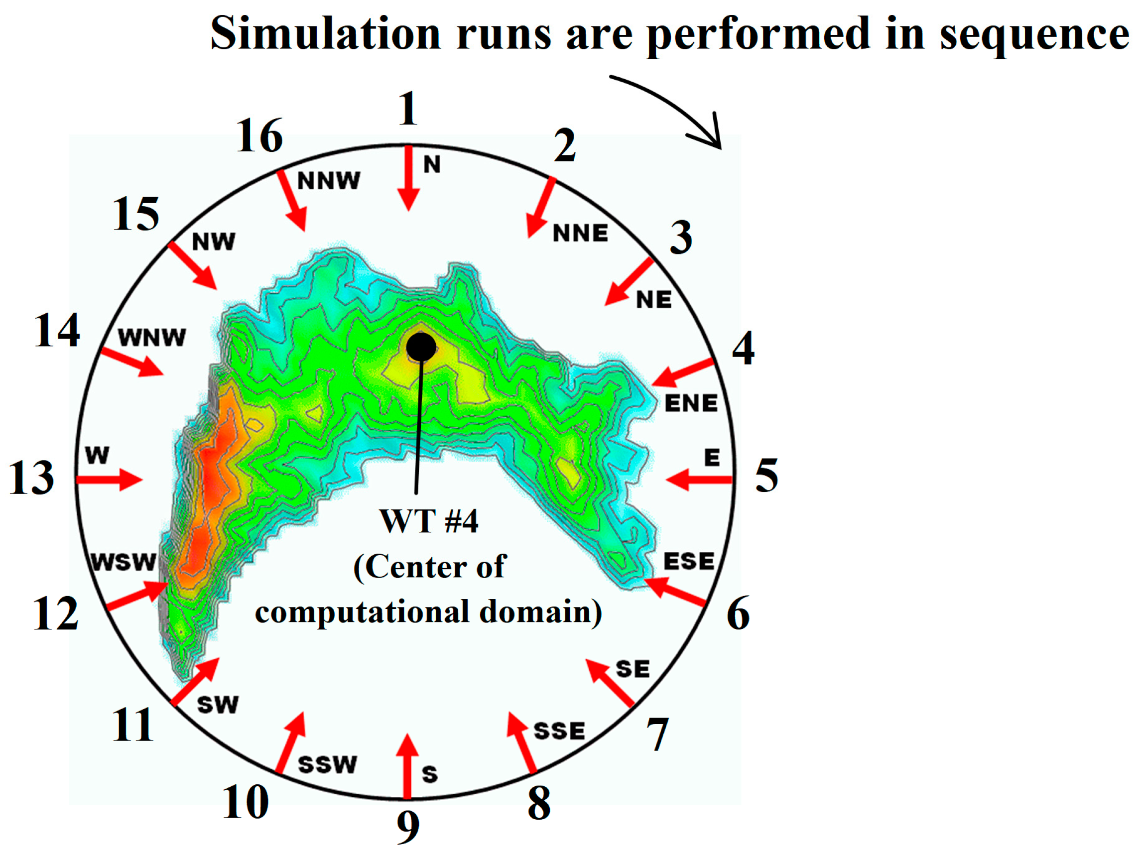
Step 1. As shown in Figure 6, wind patterns are simulated by RIAM-COMPACT for 16 individual wind directions for a prediction point. After the flow field has fully developed in a simulation run, the simulation is continued, and the time-averaged flow is calculated.
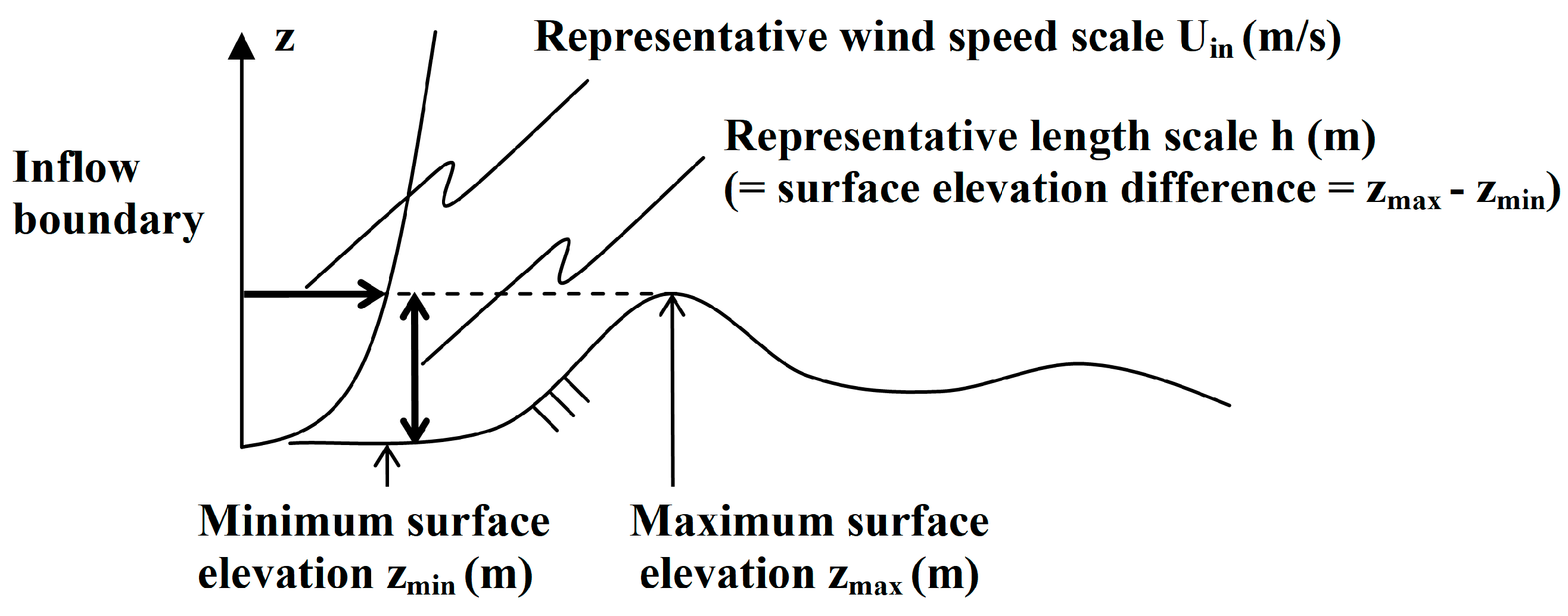
The computational domain is a square with 5 km sides with WT #4 in the center of the domain (Figure 6). The top boundary of the computational domain is set to 700 m. Terrain features are reconstructed with the use of high-resolution (5 m horizontal spatial resolution) surface elevation data. The numbers of computational grid cells are 51 (streamwise (x)) × 51 (spanwise (y)) × 41 (vertical (z)). Variable grid pacing is used in the x- and y-directions so that the grid density increases toward the center of the domain. Likewise, variable grid spacing is used in the z-direction so that grid density is highest near the ground surface. The vertical height of the first layer of grid cells, that is the minimum vertical grid height, is approximately 2.5 m. A vertical profile of wind speed based on the 1/7 power law is given for the inflow boundary. The free-slip condition is set for the side and upper boundaries. The convective outflow condition is applied to the outflow boundary. On the ground, the no-slip condition is imposed. The non-dimensional parameter, Re, in Equation (2), defined as Uin h/ν, is the Reynolds number and is set to 104. Here, h indicates the difference between the minimum and maximum surface elevations within the computational domain (h = 143 m). Uin represents the wind speed at the inflow boundary at the height of the maximum surface elevation in the computational domain, and ν is the coefficient of kinematic viscosity. The representative scales used for the present simulations, h and Uin, are shown in Figure 7. The time step in the model is set to ∆t = 2 × 10⁻³ h/Uin.
Step 2. For each inflow direction (Figure 6), the ratio of the simulated hub-height wind speed at a prediction point to the simulated wind speed at the height of an observation pole, that is, at the reference point, is computed, yielding a set of 16 wind speed ratios for the prediction point. The value of the wind speed at the reference point is normalized as “1”. In this step, the wind direction set at the inflow boundary is assumed to match that at the reference point. In the present study, points located at WT #4 and WT #6 at the hub-height are used as the reference points (hereafter, in the context of reference points, these reference points will be referred to as WT #4 and WT #6). Thus, the following wind speed ratios are evaluated: WT #1/WT #4, …, WT #10/WT #4; WT #1/WT #6, …, WT #10/WT #6. To compute these wind speed ratios, the scalar wind speed, VEL, is used in both the denominator and numerator and is computed from the time-averaged wind velocity components in the x- and y-directions. Here, the physical quantity referred to as VEL is defined as follows:
Step 3. The observed time-series of the scalar wind speed at the reference point is converted to a time-series of scalar wind speed at a prediction point as follows. According to the wind direction at the reference point at a given instance in the observed time-series, the scalar wind speed at the reference point is multiplied by the wind speed ratio, which was determined beforehand for the prediction point for that wind direction in Step 2. By applying this operation to an observed time-series of scalar wind speeds that extends over a period of one year or any period of interest and processing the outcome of the operation statistically, the monthly and annual average wind speed can be obtained for an arbitrary prediction point.
5. Results and Discussion
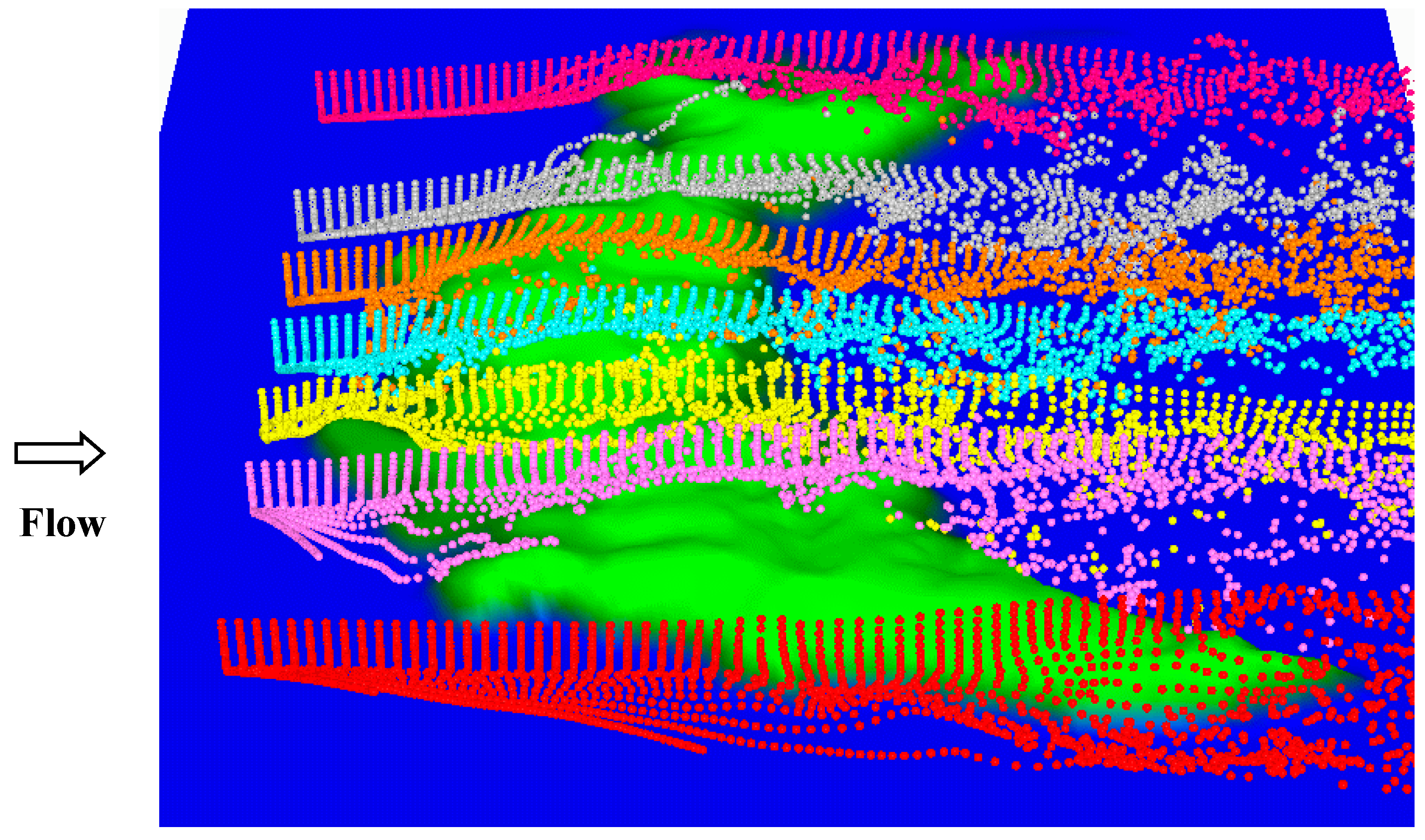
Figure 8 illustrates instantaneous views of flows that were visualized with the passive particle tracking method. The inflow wind direction for this case is northerly. This figure indicates that, due to the influence of the terrain irregularities, wind speed and direction change in complex ways as the wind flows over Cape Noma. In the procedure for predicting the actual wind speed that is proposed in the present study, simulations are run until fully-developed flows, as the one illustrated in Figure 8, are achieved, and the simulations are continued for a period of time. Then, the results of the simulations are used to obtain the time-averaged flow field.
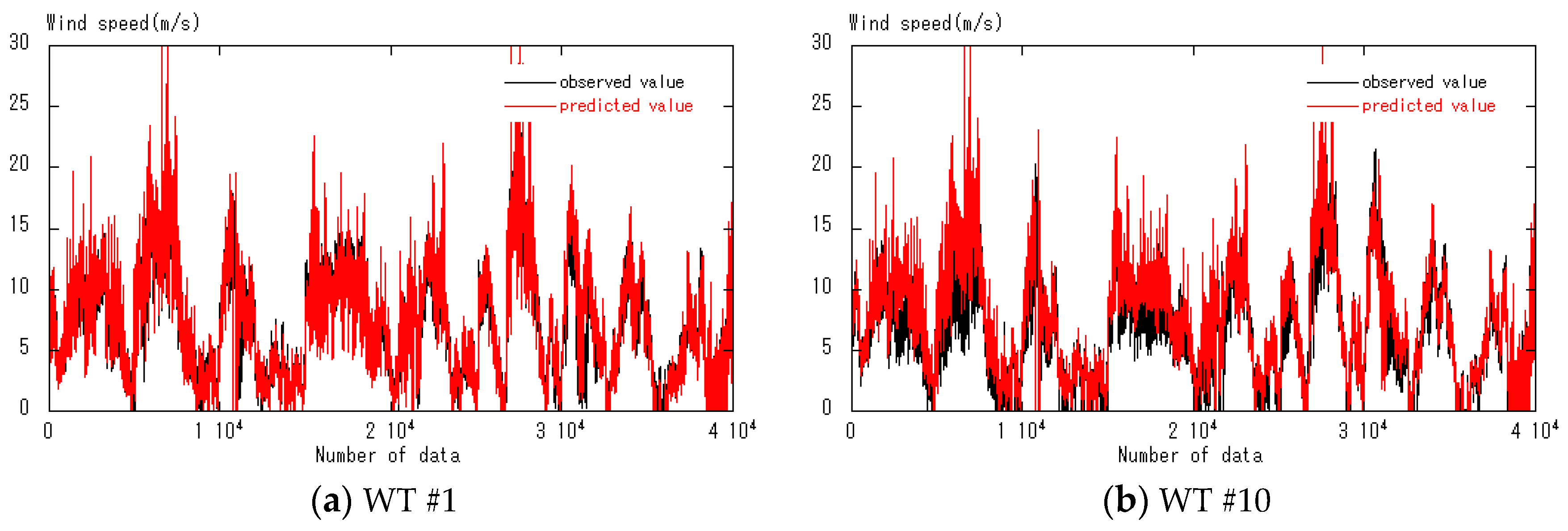
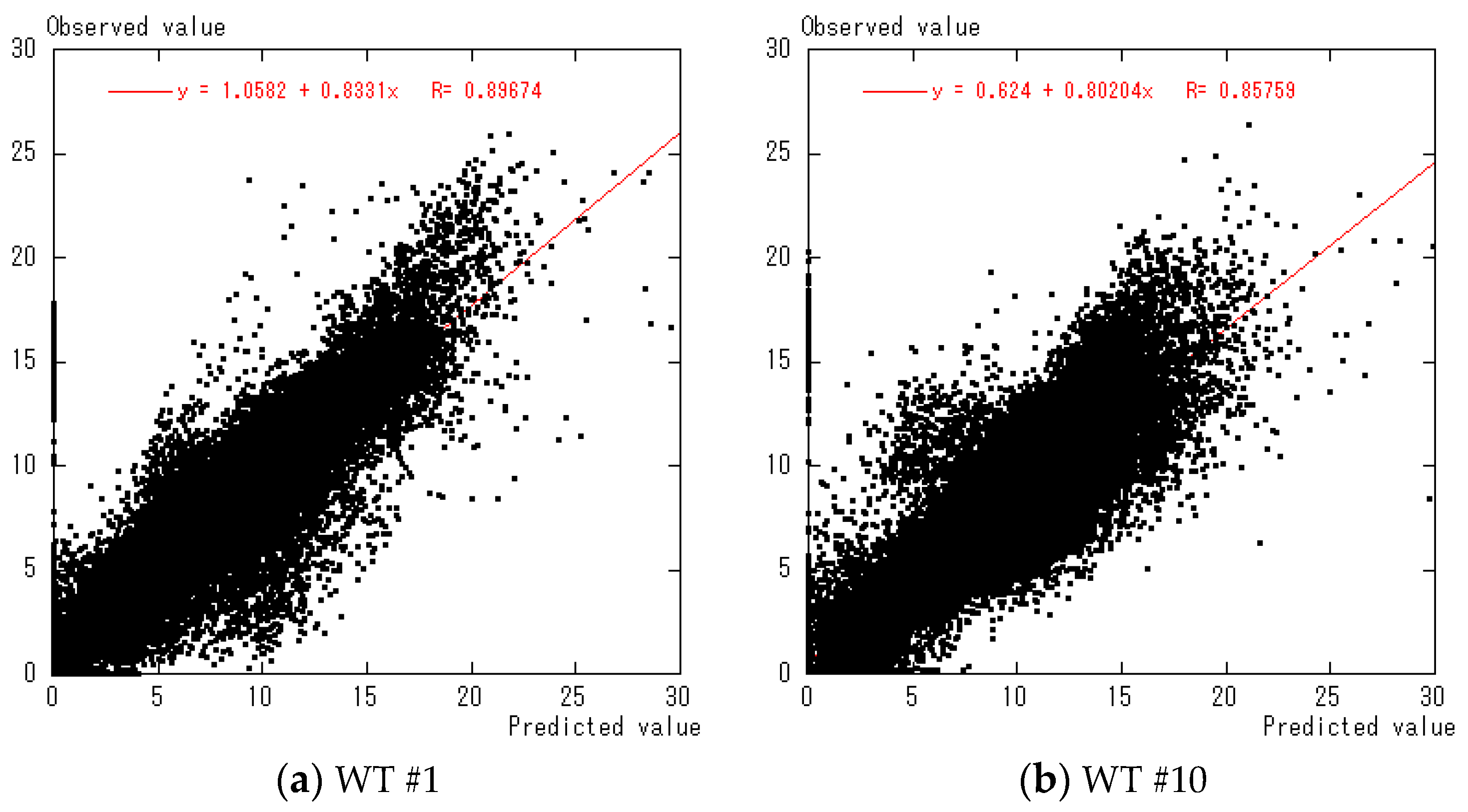
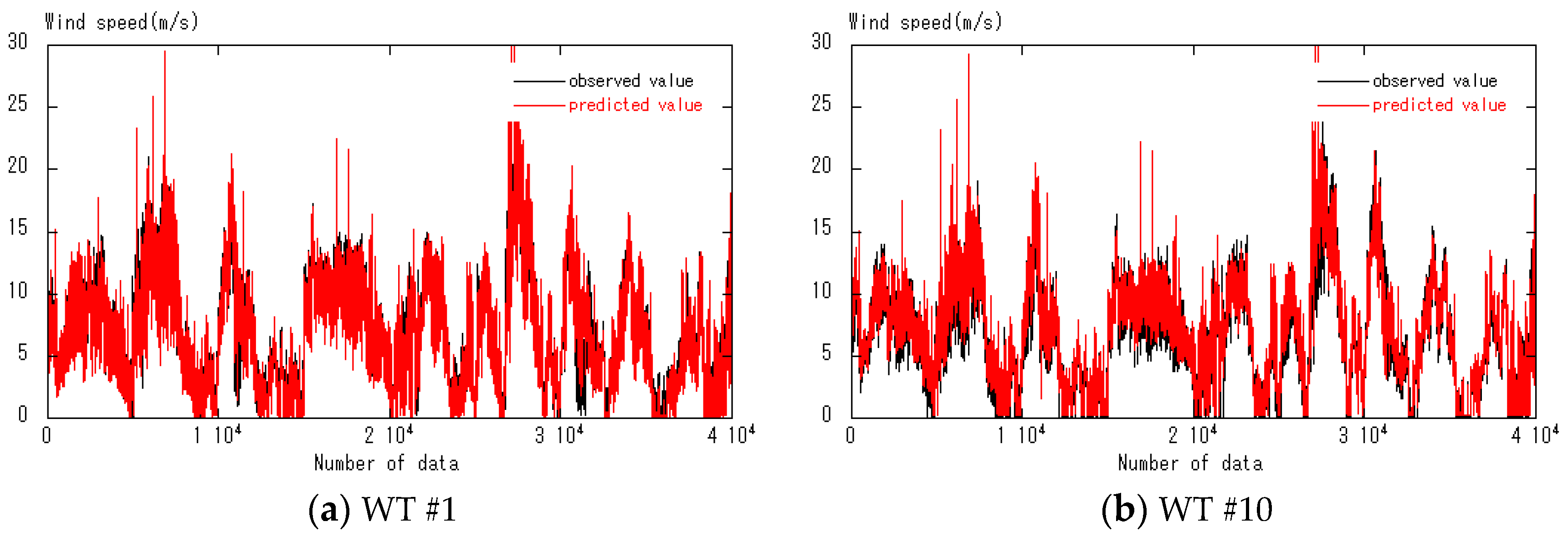
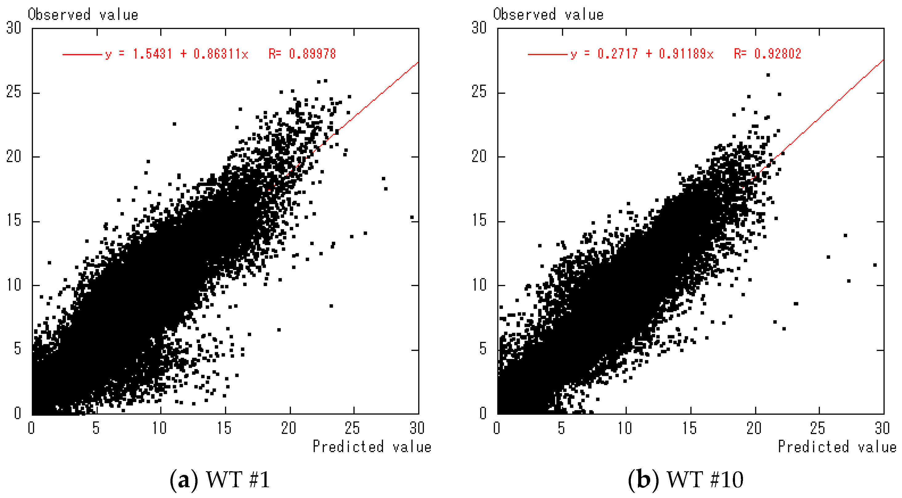
Figure 9 shows comparisons of the observed and predicted time-series of scalar wind speed for the hub-height of WT #1 and WT #10. To obtain the predicted scalar wind speed in this figure, WT #4 was used as the reference point. Figure 10 shows scatter plots of the observed and predicted scalar wind speed from Figure 9. Figure 11 also shows comparisons of the observed and predicted time-series of scalar wind speed for the hub-height of WT #1 and WT #10; however, WT #6 was used as the reference point for the prediction of the scalar wind speed. Scatter plots for the data in Figure 11 are shown in Figure 12. In both the case of using WT #4 and the case of using WT #6 as the reference points, the proposed procedure for predicting the actual wind speed yielded predicted values that agree well with the observed values.
Table 3 summarizes the comparisons of observed and predicted values of wind speed for the cases of adopting WT #4 and WT #6 as the reference points. Table 4 gives the horizontal separation distance between a given WT and WT #4 or WT #6, both of which were used as reference points. Similarly, Table 5 shows the elevation difference between the hub-height of a given WT and reference point WT #4 or WT #6. Examinations of Table 3, Table 4 and Table 5 reveal that the relative error of the wind speed at a WT predicted by the proposed actual wind speed prediction procedure is less than approximately 20% if the horizontal separation distance and elevation difference between a prediction point (the hub-height of a WT) and the reference point are approximately 800 m or less and 50 m or less, respectively. As expected, the observed wind speed data that are used in the present study were affected by the blade rotation since they were collected from propeller vane anemometers that were mounted on the nacelles of the WTs. However, this effect is equally present in the wind speed data that were collected at all the WTs.
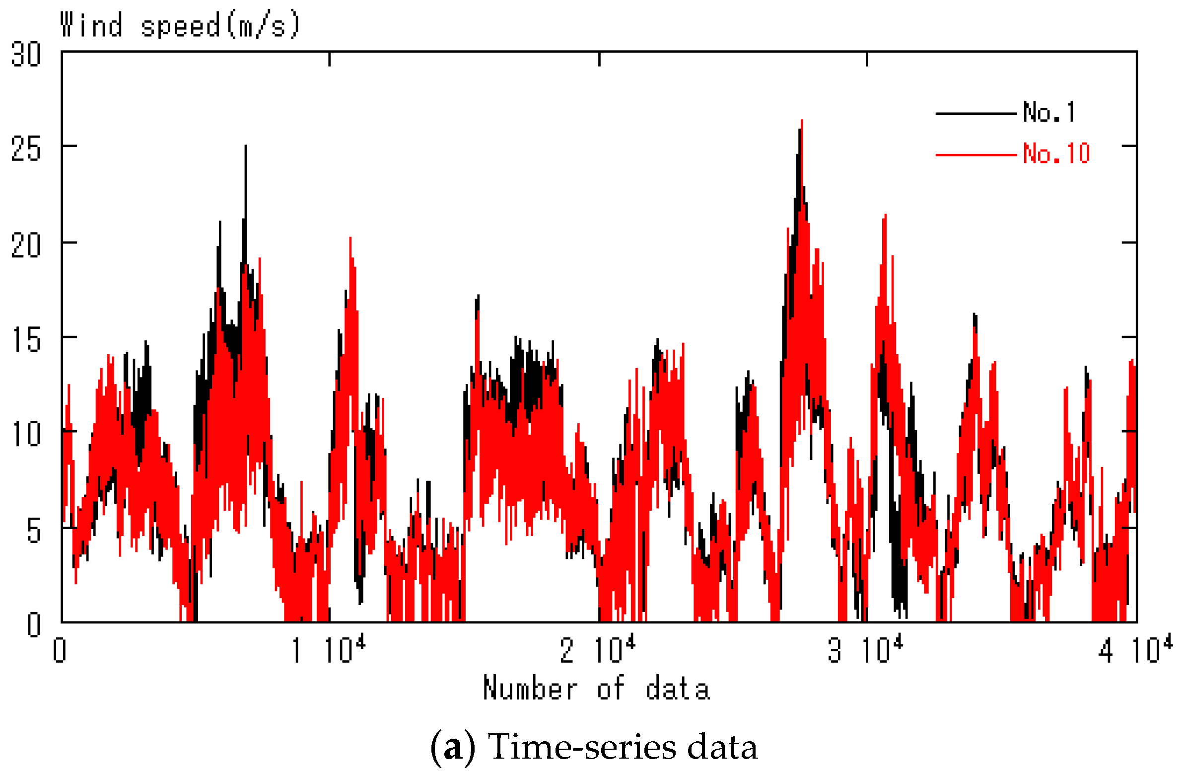
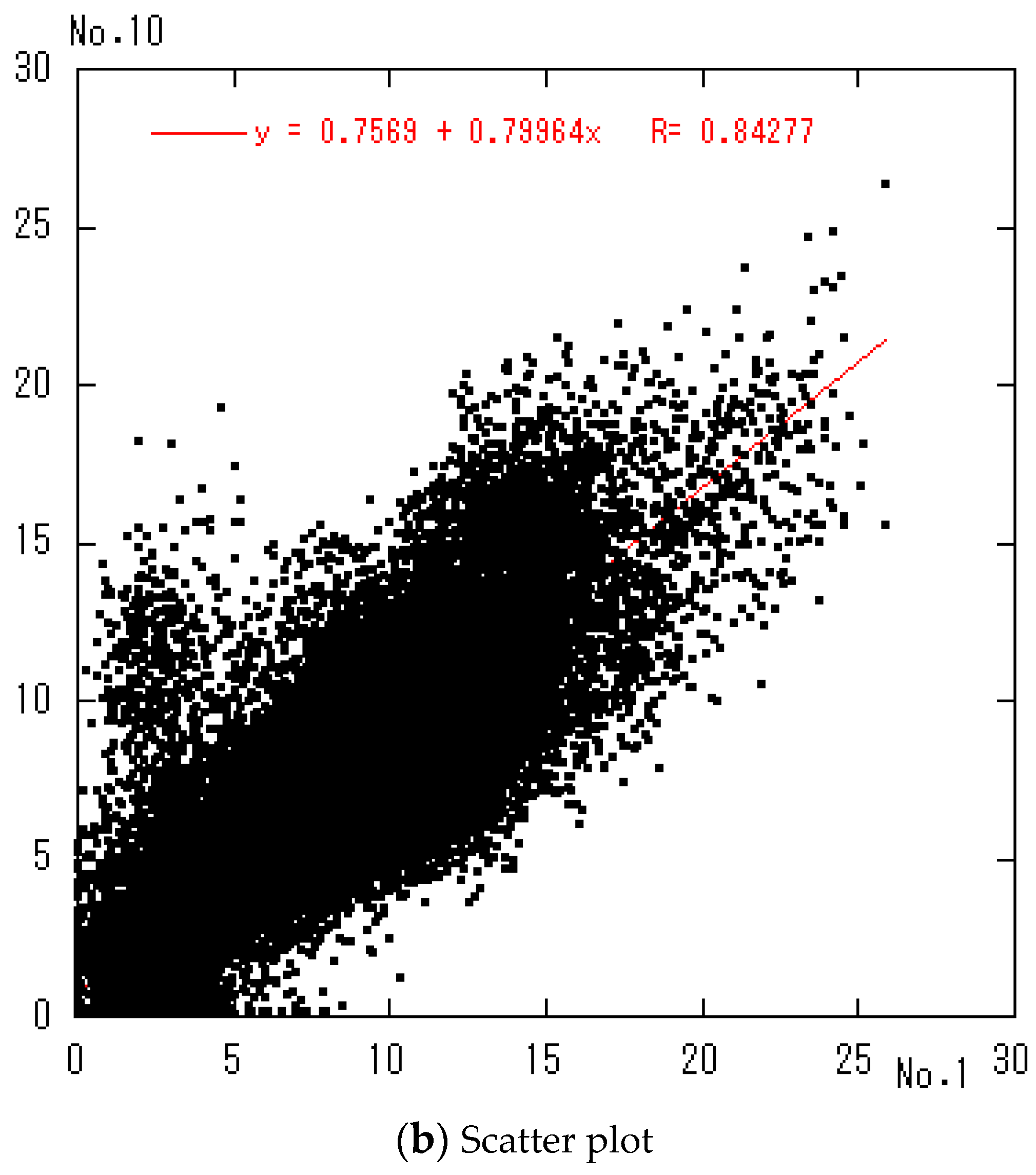
In regards to the previously discussed range of application for the proposed actual wind speed prediction procedure, the subsequent analysis examines, based on the observation data, the characteristics of airflow over complex terrain, which serve as supporting evidence for the range of application for the procedure. Figure 13 shows a comparison of the time-series of the observed wind speed from WT #1 and WT #10 and also a scatter plot of the observed wind speed from the two WTs for February 2003. The horizontal separation distance between the two WTs is as much as approximately 1200 m, and the elevation difference between the two WTs is 9 m (see Figure 2). In particular, attention should be given to the horizontal separation distance. Even though the horizontal separation distance between WT #1 and WT #10 is more than 1000 m, the temporal changes of the wind speed over the course of one month at WT #1 and WT #10 are quite similar. The correlation coefficient between the two datasets plotted in Figure 13b is 0.84.
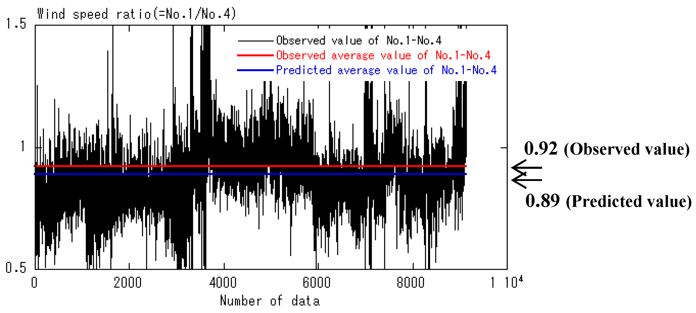
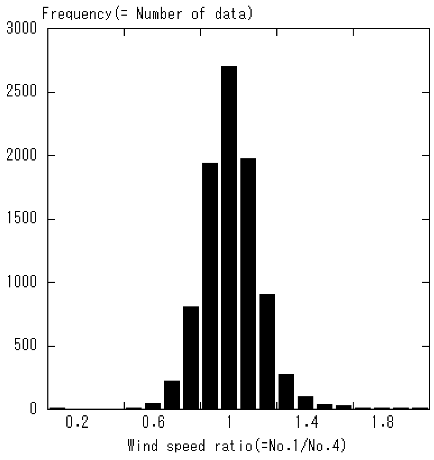
Of the 40,047 values of the ratio of the wind speed at WT #1 (the prediction point) to the wind speed at WT #4 (the reference point) for February 2003, data values only from the time of northerly wind are extracted in order to study the statistical properties of the wind speed ratio. The number of extracted data values is 9501, which corresponds to approximately 24% of the entire set of data values. In this analysis, an angle of 0° denotes wind that blows from north to south, and wind that flows from wind directions that are 348.75° or larger and 11.25°or smaller are defined as northerly wind. Figure 14 shows the time-series of the wind speed ratio only for times of northerly wind. Figure 14 also shows the average value of the observed wind speed ratios for northerly wind and that from the CFD model, revealing that these two average values agree closely. Figure 15 shows the frequency distribution of the wind speed ratios plotted in Figure 14. The frequency is distributed nearly symmetrically with the average wind speed ratio in the center. Thus, it can be said that time-series data of scalar wind speed at an arbitrary point can be obtained with the use of observed time-series of wind speed from the reference point if, with the use of CFD, the effects of terrain irregularities on the wind flow can be simulated accurately and the ratio of the wind speed at the prediction point to the wind speed at the reference point can be estimated with high accuracy.
6. Conclusions
In the present study, a procedure for predicting the actual wind speed over complex terrain was proposed. This procedure utilizes both time-series of observation data and CFD output obtained from the unsteady, nonlinear wind simulator RIAM-COMPACT, in which a collocated grid in a general curvilinear coordinate system is adopted. In this procedure, time-series of scalar wind speed obtained from field observations are converted to the actual scalar wind speed with the use of (non-dimensional) wind speed parameters that were obtained beforehand with the use of the CFD. The proposed prediction procedure was validated with the use of observation data acquired with anemometers mounted on the nacelles of wind turbines in Noma Wind Park, Kagoshima Prefecture, Japan. As for the result, the following was found for Noma Wind Park, which was investigated in the present study. If the horizontal separation distance between a prediction point and the reference point is approximately 800 m or less and the elevation difference between the two locations is 50 m or less, the relative error of the wind speed predicted by the proposed wind speed prediction procedure is less than approximately 20%. However, additional validation is necessary in regards to how the reference location is selected and the types of observation instruments used at the reference point. In addition, validation also needs to be carried out at other sites. These validations will be topics of future research. Finally, if the proposed procedure is further expanded so that it utilizes output from a meteorological model instead of observation data, a so-called real-time forecasting, which can predict wind flows a few hours to a few days into the future, will be made possible.
Funding
This research was supported by JSPS KAKENHI Grant Number 17H02053.
Acknowledgments
For conducting this research, the author was provided with the various types of data on the Noma Wind Park, Kagoshima Prefecture, Japan, by Kyushu Electric Power Co., Inc. The author would like to express his gratitude to all the organizations.
Conflicts of Interest
The author declares no conflict of interest.
References
- Palma, J.M.L.M.; Castro, F.A.; Ribeiro, L.F.; Rodrigues, A.H.; Pinto, A.P. Linear and nonlinear models in wind resource assessment and wind turbine micro-siting in complex terrain. J. Wind Eng. Ind. Aerodyn. 2008, 96, 2308–2326. [Google Scholar] [CrossRef] [Green Version]
- Berg, J.; Mann, J.; Bechmann, A.; Courtney, M.S.; Jørgensen, H.E. The Bolund experiment, part I: Flow over a steep, three-dimensional hill. Bound.-Layer Meteorol. 2011, 141, 219–243. [Google Scholar] [CrossRef]
- Bechmann, A.; Sørensen, N.N.; Berg, J.; Mann, J.; Réthoré, P.-E. The Bolund experiment, part II: Blind comparison of microscale flow models. Bound.-Layer Meteorol. 2011, 141, 245–271. [Google Scholar] [CrossRef]
- Prospathopoulos, J.M.; Politis, E.S.; Chaviaropoulos, P.K. Application of a 3D RANS solver on the complex hill of Bolund and assessment of the wind flow predictions. J. Wind Eng. Ind. Aerodyn. 2012, 107, 149–159. [Google Scholar] [CrossRef]
- Diebold, M.; Higgins, C.; Fang, J.; Bechmann, A.; Parlange, M.B. Flow over hills: A large-eddy simulation of the Bolund case. Bound.-Layer Meteorol. 2013, 148, 177–194. [Google Scholar] [CrossRef]
- Porté-Agel, F.; Wu, Y.-T.; Chen, C.-H. A Numerical Study of the Effects of Wind Direction on Turbine Wakes and Power Losses in a Large Wind Farm. Energies 2013, 6, 5297–5313. [Google Scholar] [CrossRef] [Green Version]
- Yeow, T.S.; Cuerva, A.; Conan, B.; Pérez-Álvarez, J. Wind tunnel analysis of the detachment bubble on Bolund Island. J. Phys. Conf. Ser. 2014, 555, 012021. [Google Scholar] [CrossRef]
- Yeow, T.S.; Cuerva-Tejero, A.; Pérez-Álvarez, J. Reproducing the Bolund experiment in wind tunnel. Wind Energy 2015, 18, 153–169. [Google Scholar] [CrossRef]
- Chaudhari, A.; Hellsten, A.; Hämäläinen, J. Full-Scale Experimental Validation of Large-Eddy Simulation of Wind Flows over Complex Terrain: The Bolund Hill. Adv. Meteorol. 2016. [Google Scholar] [CrossRef]
- Conan, B.; Chaudhari, A.; Aubrun, S.; van Beeck, J.; Hämäläinen, J.; Hellsten, A. Experimental and numerical modelling of flow over complex terrain: The Bolund hill. Bound.-Layer Meteorol. 2016, 158, 183–208. [Google Scholar] [CrossRef]
- Sessarego, M.; Shen, W.Z.; van der Laan, M.P.; Hansen, K.S.; Zhu, W.J. CFD Simulations of Flows in a Wind Farm in Complex Terrain and Comparisons to Measurements. Appl. Sci. 2018, 8, 788. [Google Scholar] [CrossRef]
- Astolfi, D.; Castellani, F.; Terzi, L. A Study of Wind Turbine Wakes in Complex Terrain through RANS Simulation and SCADA Data. J. Sol. Energy Eng. 2018, 140, 031001. [Google Scholar] [CrossRef]
- Uchida, T. LES Investigation of Terrain-Induced Turbulence in Complex Terrain and Economic Effects of Wind Turbine Control. Energies 2018, 11, 1530. [Google Scholar] [CrossRef]
- Uchida, T. Computational Fluid Dynamics (CFD) Investigation of Wind Turbine Nacelle Separation Accident over Complex Terrain in Japan. Energies 2018, 11, 1485. [Google Scholar] [CrossRef]
- Uchida, T.; Ohya, Y. Latest Developments in Numerical Wind Synopsis Prediction Using the RIAM-COMPACT CFD Model-Design Wind Speed Evaluation and Wind Risk (Terrain-Induced Turbulence) Diagnostics in Japan. Energies 2011, 4, 458–474. [Google Scholar] [CrossRef]
- Uchida, T. Large-Eddy Simulation and Wind Tunnel Experiment of Airflow over Bolund Hill. Open J. Fluid Dyn. 2018, 8, 30–43. [Google Scholar] [CrossRef]
- Uchida, T. High-Resolution LES of Terrain-Induced Turbulence around Wind Turbine Generators by Using Turbulent Inflow Boundary Conditions. Open J. Fluid Dyn. 2017, 7, 511–524. [Google Scholar] [CrossRef]
- Uchida, T. High-Resolution Micro-Siting Technique for Large Scale Wind Farm Outside of Japan Using LES Turbulence Model. Energy Power Eng. 2017, 9, 802–813. [Google Scholar] [CrossRef]
- Uchida, T. CFD Prediction of the Airflow at a Large-Scale Wind Farm above a Steep, Three-Dimensional Escarpment. Energy Power Eng. 2017, 9, 829–842. [Google Scholar] [CrossRef]
- Uchida, T.; Ohya, Y. Verification of the Prediction Accuracy of Annual Energy Output at Noma Wind Park by the Non-Stationary and Non-Linear Wind Synopsis Simulator, RIAM-COMPACT. J. Fluid Sci. Technol. 2008, 3, 344–358. [Google Scholar] [CrossRef]
- Uchida, T.; Ohya, Y. Micro-siting Technique for Wind Turbine Generators by Using Large-Eddy Simulation. J. Wind Eng. Ind. Aerodyn. 2008, 96, 2121–2138. [Google Scholar] [CrossRef]
- Uchida, T.; Maruyama, T.; Ohya, Y. New Evaluation Technique for WTG Design Wind Speed using a CFD-model-based Unsteady Flow Simulation with Wind Direction Changes. Model. Simul. Eng. 2011. [Google Scholar] [CrossRef]
- Kim, J.; Moin, P. Application of a fractional-step method to incompressible Navier-Stokes equations. J. Comput. Phys. 1985, 59, 308–323. [Google Scholar] [CrossRef]
- Kajishima, T. Upstream-shifted interpolation method for numerical simulation of incompressible flows. Bull. Jpn. Soc. Mech. Eng. B 1994, 60, 3319–3326. (In Japanese) [Google Scholar] [CrossRef]
- Kawamura, T.; Takami, H.; Kuwahara, K. Computation of high Reynolds number flow around a circular cylinder with surface roughness. Fluid Dyn. Res. 1986, 1, 145–162. [Google Scholar] [CrossRef]
- Smagorinsky, J. General circulation experiments with the primitive equations, Part 1, Basic experiments. Mon. Weather Rev. 1963, 91, 99–164. [Google Scholar] [CrossRef]
Figure 1.
Cape Noma and surrounding topographical features.

Figure 2.
View of Noma Wind Park.

Figure 3.
Propeller vane anemometer mounted on a WT nacelle (indicated by “A”).

Figure 4.
Characteristics of wind at Noma Wind Park, WT #4, for the year from June 2002–May 2003. (a) Occurrence frequency (%); (b) annual average wind speed (m/s).
Figure 4.
Characteristics of wind at Noma Wind Park, WT #4, for the year from June 2002–May 2003. (a) Occurrence frequency (%); (b) annual average wind speed (m/s).

Figure 5.
Characteristics of wind at Noma Wind Park, WT #4, for the month of February 2003. (a) Occurrence frequency (%); (b) monthly average wind speed (m/s).
Figure 5.
Characteristics of wind at Noma Wind Park, WT #4, for the month of February 2003. (a) Occurrence frequency (%); (b) monthly average wind speed (m/s).

Figure 6.
Conceptual outline of wind simulations for 16 wind directions for Noma Wind Park.

Figure 7.
Representative scales used in the present study.

Figure 8.
Examples of flows visualized with the passive particle tracking method, northerly wind, bird’s eye view.
Figure 8.
Examples of flows visualized with the passive particle tracking method, northerly wind, bird’s eye view.

Figure 9.
Time-series data of observed and predicted wind speed, reference point: WT #4.

Figure 10.
Scatter plots of observed and predicted wind speed, reference point: WT #4.

Figure 11.
Time-series data of observed and predicted wind speed, reference point: WT #6.

Figure 12.
Scatter plots of observed and predicted wind speed, reference point: WT #6.

Figure 13.
Comparison of hub-height wind speed at WT #1 and WT #10, observation data.


Figure 14.
Observed time-series of the ratio of the hub-height wind speed at WT #1 to that at WT #4, only for times of northerly wind, February 2003.
Figure 14.
Observed time-series of the ratio of the hub-height wind speed at WT #1 to that at WT #4, only for times of northerly wind, February 2003.

Figure 15.
Frequency distribution of the ratio of the hub-height wind speed at WT #1 to that at WT #4, only for times of northerly wind, February 2003.
Figure 15.
Frequency distribution of the ratio of the hub-height wind speed at WT #1 to that at WT #4, only for times of northerly wind, February 2003.


Table 1.
Specifications of wind turbines (WTs) at Noma Wind Park.
| Item | WT #1–#5 | WT #6–#10 |
|---|---|---|
| Output | 300 kW/WT | |
| Generator type | Induction | Synchronous |
| Cut-in speed | 3.5 m/s | 2.5 m/s |
| Rated wind speed | 14.4 m/s | 14.0 m/s |
| Cut-out speed | 24 m/s | 25 m/s |
| Rotor diameter | 29 m | 30 m |
| Tower height | 30 m (WT #4:45 m) | 30 m (WT #6:45 m) |
Table 2.
WT hub-heights and surface elevations.
| Number | Hub-Height (Tower Height) | Surface Elevation of WT Site |
|---|---|---|
| WT #1 | 30 m | 100 m |
| WT #2 | 92 m | |
| WT #3 | 109 m | |
| WT #4 | 45 m | 122 m |
| WT #5 | 30 m | 102 m |
| WT #6 | 45 m | 117 m |
| WT #7 | 30 m | 88 m |
| WT #8 | 95 m | |
| WT #9 | 92 m | |
| WT #10 | 109 m |
Table 3.
Comparisons of observed and predicted values of wind speed.
| (a) Reference Point: WT #4 | ||||
| February 2003 | Observed Wind Speed (m/s) | Predicted Wind Speed (m/s) | Relative Error (%) | Correlation Coefficient |
| WT #1 | 7.27 | 7.45 | 2.56 | 0.90 |
| WT #2 | 7.07 | 7.24 | 2.31 | 0.89 |
| WT #3 | 7.91 | 7.60 | 3.92 | 0.93 |
| WT #5 | 7.11 | 7.45 | 4.84 | 0.91 |
| WT #6 | 7.39 | 7.83 | 5.90 | 0.92 |
| WT #7 | 6.35 | 7.06 | 11.28 | 0.83 |
| WT #8 | 6.78 | 7.40 | 9.09 | 0.90 |
| WT #9 | 6.17 | 7.20 | 16.62 | 0.84 |
| WT #10 | 6.57 | 7.41 | 12.84 | 0.86 |
| Average | 6.96 | 7.40 | 6.42 | 0.89 |
| (b) Reference Point: WT #6 | ||||
| February 2003 | Observed Wind Speed (m/s) | Predicted Wind Speed (m/s) | Relative Error (%) | Correlation Coefficient |
| WT #1 | 7.27 | 6.63 | 8.74 | 0.90 |
| WT #2 | 7.07 | 6.32 | 10.71 | 0.87 |
| WT #3 | 7.91 | 6.48 | 18.09 | 0.92 |
| WT #5 | 7.11 | 7.73 | 6.80 | 0.92 |
| WT #6 | 7.39 | 7.07 | 0.54 | 0.92 |
| WT #7 | 6.35 | 6.80 | 7.10 | 0.92 |
| WT #8 | 6.78 | 7.02 | 3.58 | 0.96 |
| WT #9 | 6.17 | 6.80 | 10.22 | 0.92 |
| WT #10 | 6.57 | 6.90 | 5.13 | 0.93 |
| Average | 6.96 | 6.86 | 2.73 | 0.92 |
Table 4.
Horizontal separation distance between a given WT and the reference point.
| Reference Point: WT #4 | Horizontal Separation Distance (m) | Reference Point: WT #6 | Horizontal Separation Distance (m) |
|---|---|---|---|
| WT #1–WT #4 | approx. 560 | WT #1–WT #6 | approx. 760 |
| WT #2–WT #4 | approx. 280 | WT #2–WT #6 | approx. 530 |
| WT #3–WT #4 | approx. 140 | WT #3–WT #6 | approx. 350 |
| WT #5–WT #4 | approx. 180 | WT #4–WT #6 | approx. 300 |
| WT #6–WT #4 | approx. 300 | WT #5–WT #6 | approx. 140 |
| WT #7–WT #4 | approx. 420 | WT #7–WT #6 | approx. 140 |
| WT #8–WT #4 | approx. 430 | WT #8–WT #6 | approx. 240 |
| WT #9–WT #4 | approx. 630 | WT #9–WT #6 | approx. 350 |
| WT #10–WT #4 | approx. 800 | WT #10–WT #6 | approx. 500 |
Table 5.
Elevation difference between the hub-height of a given WT (a prediction point) and the reference point.
Table 5.
Elevation difference between the hub-height of a given WT (a prediction point) and the reference point.
| Reference Point: WT #4 | Elevation Difference (m) | Reference Point: WT #6 | Elevation Difference (m) |
|---|---|---|---|
| WT #1–WT #4 | 37 | WT #1–WT #6 | 32 |
| WT #2–WT #4 | 45 | WT #2–WT #6 | 40 |
| WT #3–WT #4 | 28 | WT #3–WT #6 | 23 |
| WT #5–WT #4 | 35 | WT #4–WT #6 | 5 |
| WT #6–WT #4 | 5 | WT #5–WT #6 | 30 |
| WT #7–WT #4 | 49 | WT #7–WT #6 | 44 |
| WT #8–WT #4 | 42 | WT #8–WT #6 | 37 |
| WT #9–WT #4 | 45 | WT #9–WT #6 | 40 |
| WT #10–WT #4 | 28 | WT #10–WT #6 | 23 |
© 2018 by the author. Licensee MDPI, Basel, Switzerland. This article is an open access article distributed under the terms and conditions of the Creative Commons Attribution (CC BY) license (http://creativecommons.org/licenses/by/4.0/).
Share and Cite
MDPI and ACS Style
Uchida, T. Computational Fluid Dynamics Approach to Predict the Actual Wind Speed over Complex Terrain. Energies 2018, 11, 1694. https://doi.org/10.3390/en11071694
AMA Style
Uchida T. Computational Fluid Dynamics Approach to Predict the Actual Wind Speed over Complex Terrain. Energies. 2018; 11(7):1694. https://doi.org/10.3390/en11071694
Chicago/Turabian StyleUchida, Takanori. 2018. "Computational Fluid Dynamics Approach to Predict the Actual Wind Speed over Complex Terrain" Energies 11, no. 7: 1694. https://doi.org/10.3390/en11071694
Note that from the first issue of 2016, this journal uses article numbers instead of page numbers. See further details here.