Article

LES Investigation of Terrain-Induced Turbulence in Complex Terrain and Economic Effects of Wind Turbine Control

Research Institute for Applied Mechanics (RIAM), Kyushu University, 6-1 Kasuga-kouen, Kasuga, Fukuoka 816-8580, Japan
Energies 2018, 11(6), 1530; https://doi.org/10.3390/en11061530
Submission received: 25 May 2018 / Revised: 8 June 2018 / Accepted: 10 June 2018 / Published: 12 June 2018
(This article belongs to the Collection Wind Turbines)

Abstract

:
In the present study, numerical wind simulation was conducted by reproducing the realistic topography near wind turbine sites with high spatial resolutions and using the Large-Eddy Simulation (LES) technique. The topography near wind turbine sites serves as the origin of the terrain-induced turbulence. The obtained numerical simulation results showed that the terrain-induced turbulence is generated at a small terrain feature located upstream of the wind turbine. The generated terrain-induced turbulence affects the wind turbine directly. The wind speed and wind direction at the wind turbine site are significantly changed with time. In the present study, a combination of the series of wind simulation results and on-site operation experience led to a decision to adopt an “automatic shutdown program”. Here, an “automatic shutdown program” means the automatic suspension of wind turbine operation based on the wind speed and wind direction meeting the conditions associated with significant effects of terrain-induced turbulence at a wind turbine site. The adoption of the “automatic shutdown program” has successfully led to a large reduction in the number of occurrences of wind turbine damage, in addition to, creating positive economic effects.

1. Introduction

One technical issue, which needs to be resolved in the near future in the field of wind power generation, is to establish a numerical wind prediction technique, which allows; (1) accurate wind resource assessment for wind turbine micro-siting [1,2,3,4], and (2) identification of local wind risks to wind turbines, such as wind turbine wake [5,6] and terrain-induced turbulence [7,8,9,10,11,12,13,14,15].
The numerical wind prediction technique, RIAM-COMPACT (Research Institute for Applied Mechanics, Kyushu University, COMputational Prediction of Airflow over Complex Terrain), which has been developed by the authors’ research group, has a potential to resolve the above-mentioned issue all at once [7,8,9,10,11,12,13,14,15]. The core technology of the RIAM-COMPACT is under continuous development at the Research Institute for Applied Mechanics (RIAM), Kyushu University.
Recently, it has been reported that the availability factors of wind turbines on wind farms situated on complex terrain fall short of those originally projected; that is, reports of damage and breakage of the exteriors and interiors of wind turbines (e.g., breakage of yaw motors and yaw gears, and cracks on wind turbine blades), as well as wind turbines with, notably, low power output have surfaced. The main cause of these problems is that small variations in the topographical relief in the vicinity of wind turbines serve as the origin of turbulence (terrain-induced turbulence). The present paper will discuss a specific example of a wind-risk (terrain-induced turbulence) diagnosis using the RIAM-COMPACT natural terrain version software (Large-Eddy Simulation (LES) modeling).

2. Summary of the RIAM-COMPACT Natural Terrain Version Software

In the present study, to predict airflows over real complex terrain with high accuracy, the RIAM-COMPACT natural terrain version software (LES modeling) is used [7,8,9,10,11,12,13,14,15]. The RIAM-COMPACT natural terrain version software uses collocated grids in a general curvilinear coordinate system to avoid numerical instability. In these collocated grids, the physical velocity components and pressure are defined at the cell centers and variables, which result from the contravariant velocity components multiplied by the Jacobian, are defined at the cell faces. As for the simulation technique, the Finite-Difference Method (FDM) is adopted and a Large-Eddy Simulation (LES) model is used for the turbulence model. In LES, a spatial filter is applied to the flow field to separate eddies of various scales into Grid Scale (GS) components, which are larger than the computational grid cells, and Sub-Grid Scale (SGS) components, which are smaller than the computational grid cells. Large-scale eddies, i.e., the GS components of turbulence eddies, are directly numerically simulated without relying on the use of a physically simplified model. On the other hand, the main effect of small-scale eddies, i.e., the SGS components, is to dissipate energy and this dissipation is modeled based on the physical considerations of the SGS stress.
For the governing equations of the flow, a spatially-filtered continuity equation for incompressible fluid (Equation (1)) and a spatially-filtered Navier-Stokes equation (Equation (2)) are used:
u i x i = 0
u i t + u j u i x j = p x i + 1 Re 2 u i x j x j
Supporting equations are given in Equations (3)–(8):
τ i j u i u j ¯ 1 3 u k u k ¯ δ i j 2 ν S G S S ¯ i j
ν S G S = ( C s f s Δ ) 2 | S ¯ |
| S ¯ | = ( 2 S ¯ i j S ¯ i j ) 1 / 2
S ¯ i j = 1 2 ( u ¯ i x j + u ¯ j x i )
f s = 1 e x p ( z + / 25 )
Δ = ( h x h y h z ) 1 / 3
The computational algorithm and the time marching method are based on the Fractional-Step (FS) method [16] and the Euler explicit method, respectively. The Poisson’s equation for pressure is solved by the Successive Over-Relaxation (SOR) method. For discretization of all spatial terms in Equation (2), except for the convective term, a second-order central difference scheme is applied. For the convective term, a third-order upwind difference scheme is applied. An interpolation technique based on four-point differencing and four-point interpolation by Kajishima [17] is used for the fourth-order central differencing that appears in the discretized form of the convective term. For the weighting of the numerical diffusion term in the convective term discretized by third-order upwind differencing, α = 3.0 is commonly applied in the Kawamura-Kuwahara scheme [18]. However, α = 0.5 is used in the present study to minimize the influence of numerical diffusion. For LES subgrid-scale modeling, the commonly used Smagorinsky model [19] is adopted. A wall-damping function is used with a model coefficient of 0.1.

3. Wind Synopsis Analysis with the RIAM-COMPACT Natural Terrain Version Software

As described earlier, the availability factors of wind turbines in wind farms on complex terrain often fall below the originally projected values. In other words, problems, such as wind turbines with notably low power output and damage and breakage of the exteriors and interiors of wind turbines, have surfaced. The effects of turbulence (terrain-induced turbulence) have also been made note of for the Atsumi Wind Farm in the Aichi Prefecture, Japan, the site investigated in the present study. In the present paper, an LES turbulence simulation is conducted with high spatial resolution using the RIAM-COMPACT natural terrain version software. The main purpose of this simulation is to reproduce the relative comparisons of wind conditions among wind turbine locations.

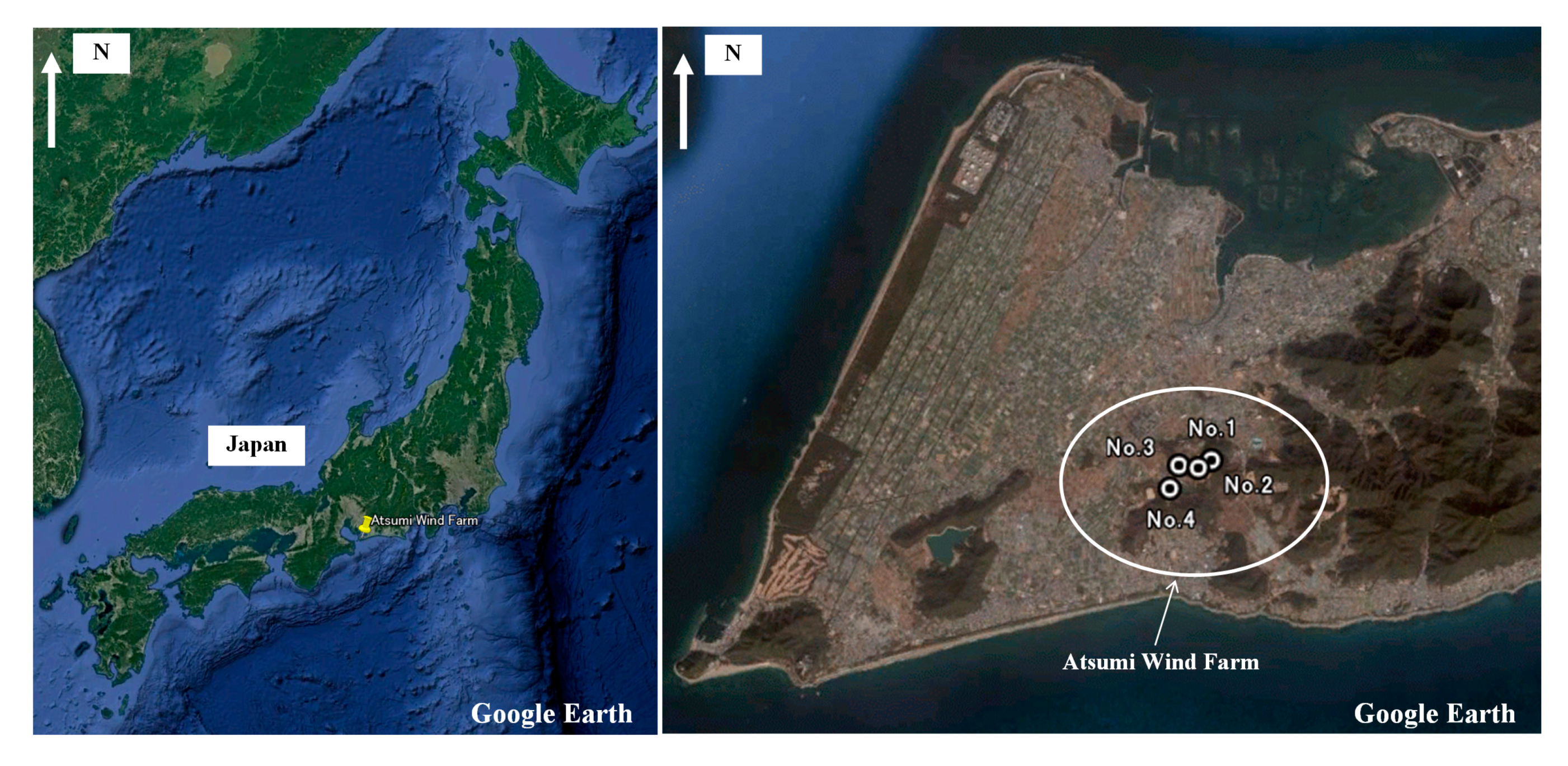
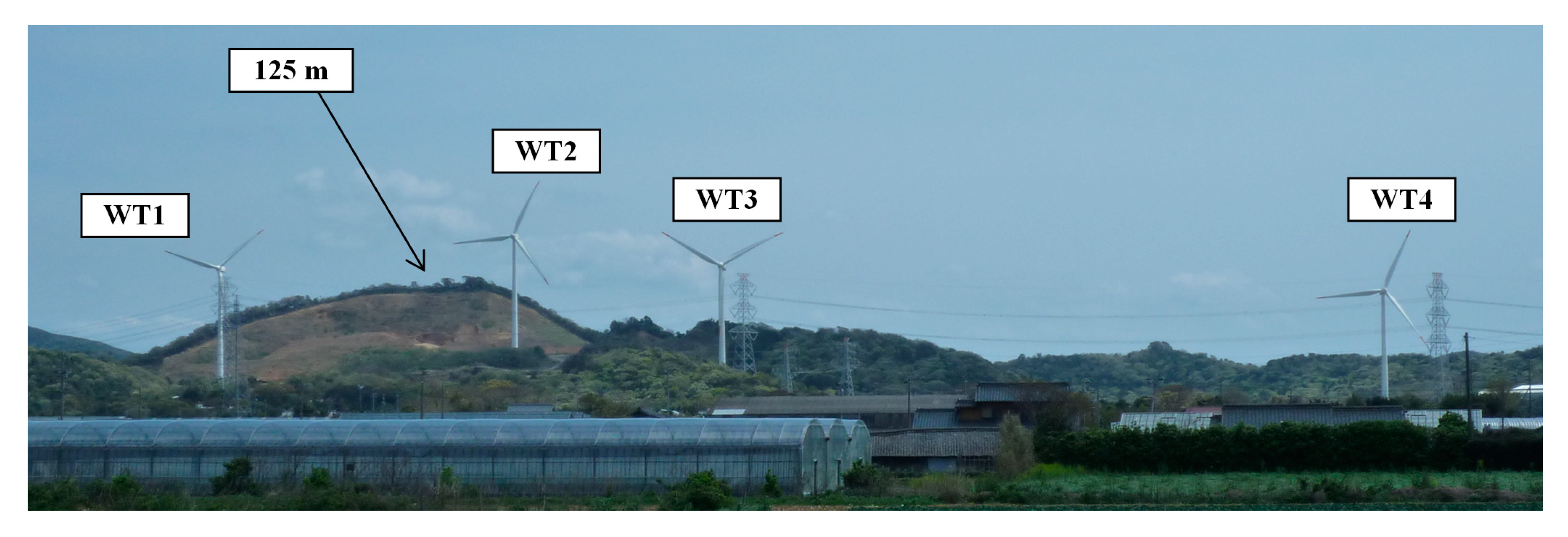
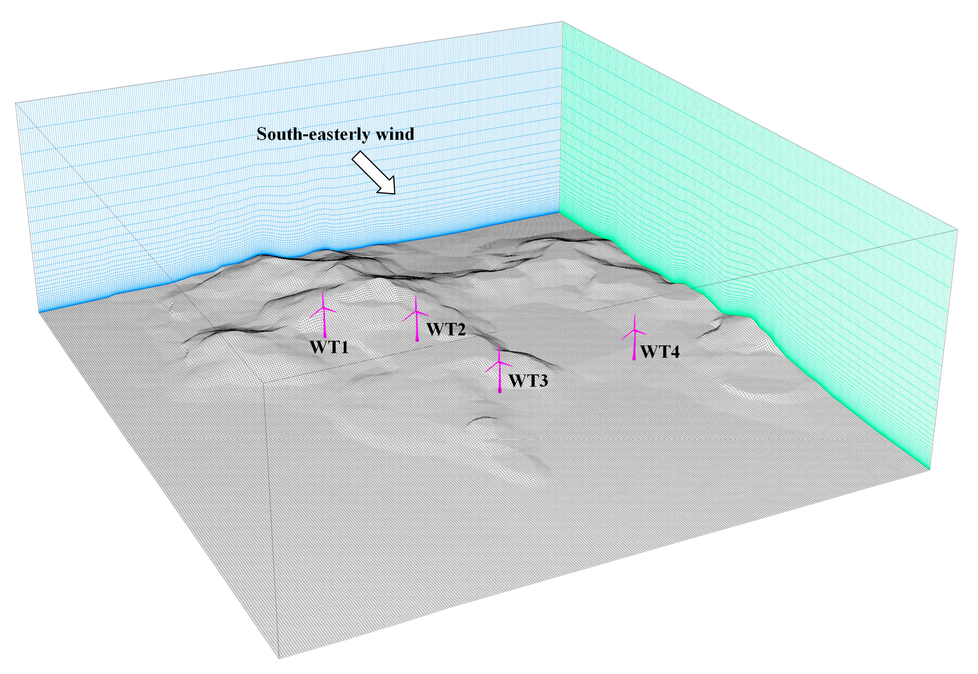
3.1. Summary of the Atsumi Wind Farm

A wind synopsis analysis was performed for the Atsumi Wind Farm (in operation since March 2007), with the cooperation of the Kyudenko Corporation (see Figure 1, Figure 2 and Figure 3 and Table 1).

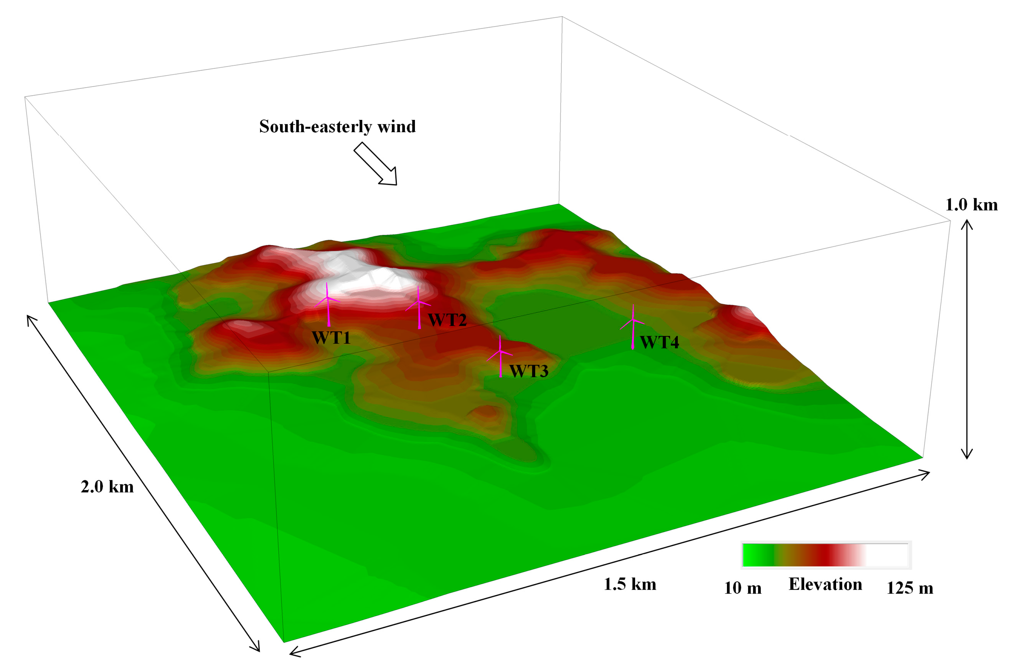
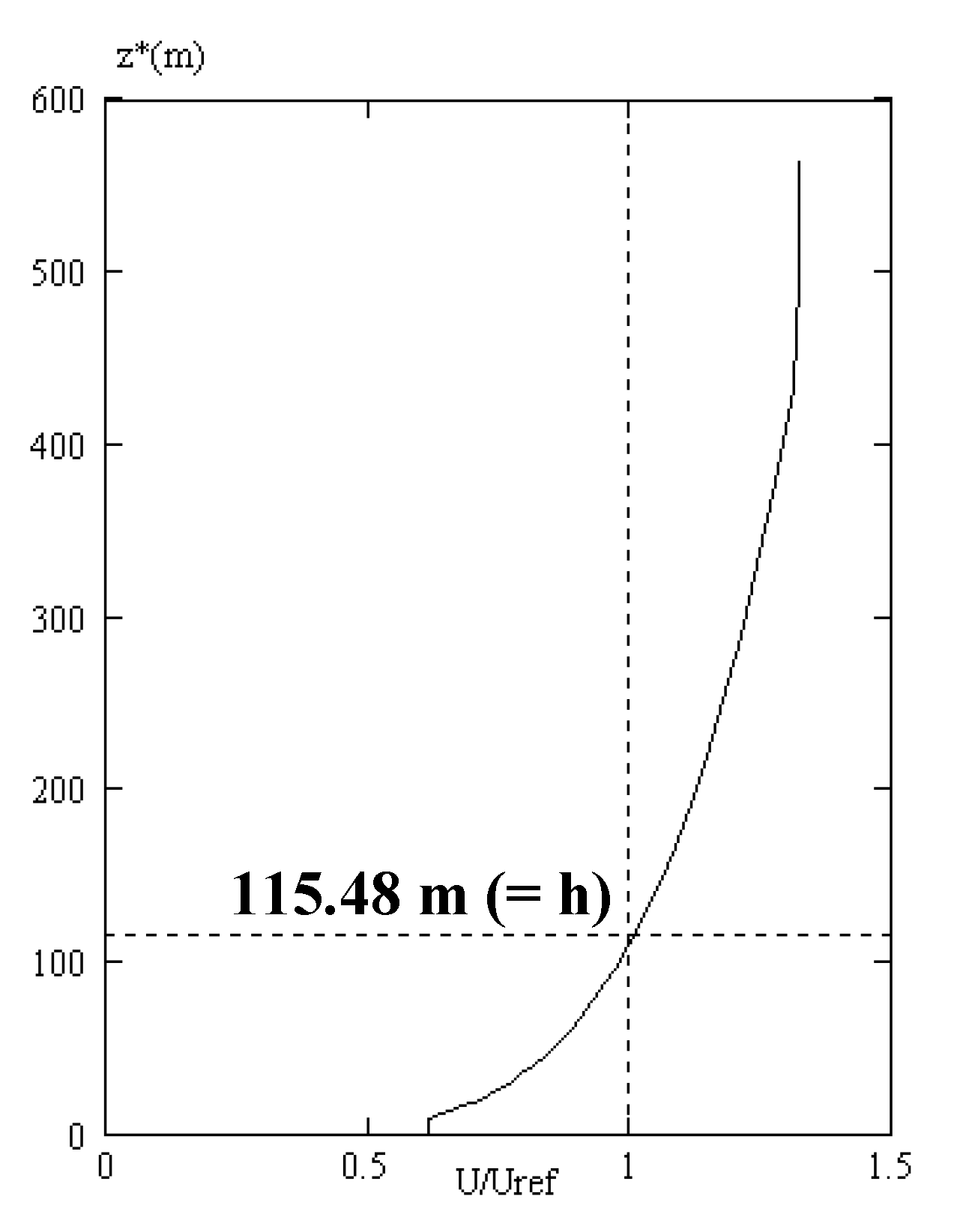
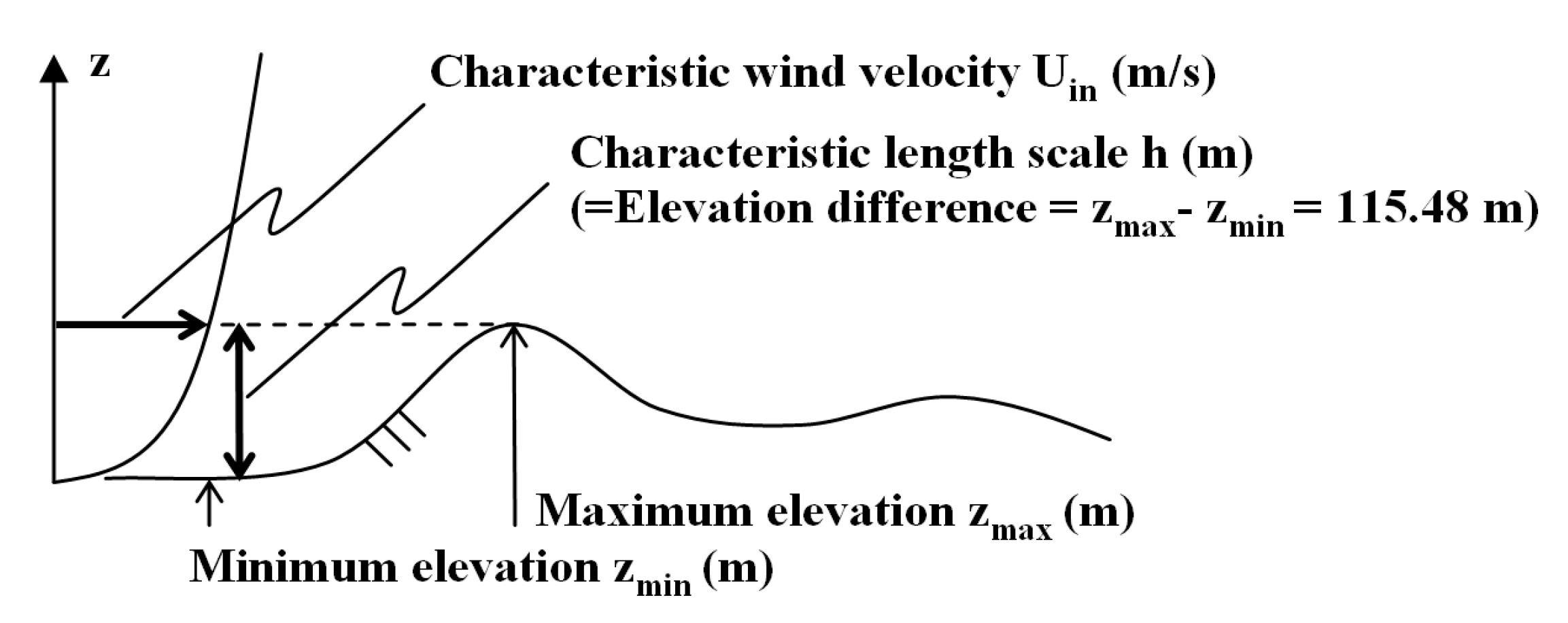
3.2. Simulation Set-Up

As shown in Figure 4, the dimensions of the computational domain are 2.0 (x) × 1.5 (y) × 1.0 (z) km, where x is the streamwise, y is the spanwise, and z is the vertical direction, respectively. A buffer zone is established in the upstream end of the computational domain in which the terrain irregularities are reduced by 97% to form flat terrain. Similarly, a buffer zone is added to the downstream end of the domain. The terrain elevation data were created with a spatial resolution of 5 m using contour lines from the basis map information of the Geospatial Information Authority of Japan (map scale 1:25,000). The total number of computational grid points, including those in the buffer zones in the upstream and downstream ends of the computational domain, are 391 (x) × 301 (y) × 41 (z), that is, approximately 4.8 million (Figure 5). The grid spacing is uniformly 5 m in both the x- and y-directions. The vertical grid spacing decreases smoothly down to 0.35 m at the ground surface.
The wind direction set in the present simulation is south-easterly, which is a wind direction associated with confirmed abnormalities of wind turbines at this site. The wind velocity profile applied at the inflow boundary is based on a commonly used empirical power law (Figure 6). A power law index is set to 5. Furthermore, at the side and upper boundaries, slip boundary conditions are applied. The convective outflow condition is applied at the outflow boundary. Non-slip boundary conditions are applied at the ground surface. The present LES is assumed to reproduce the wind tunnel testing. Therefore, the non-dimensional parameter, Re, in Equation (2) is the Reynolds number (=Uin h/ν) and is set to 104. Figure 7 illustrates the characteristic scales relevant in the present simulation: h is the difference between the minimum and maximum ground surface elevations within the computational domain, Uin is the wind speed at the inflow boundary at the maximum ground surface elevation within the computational domain, and ν is the coefficient of the dynamic viscosity of air. The time step is set to Δt = 2 × 10⁻³ h/Uin. In the present simulation, the effect of vertical thermal stratification (density stratification), which is generally present in the atmosphere, is neglected. Furthermore, the effect of surface roughness is included by reconstructing the irregularities of the terrain surface in high resolution.

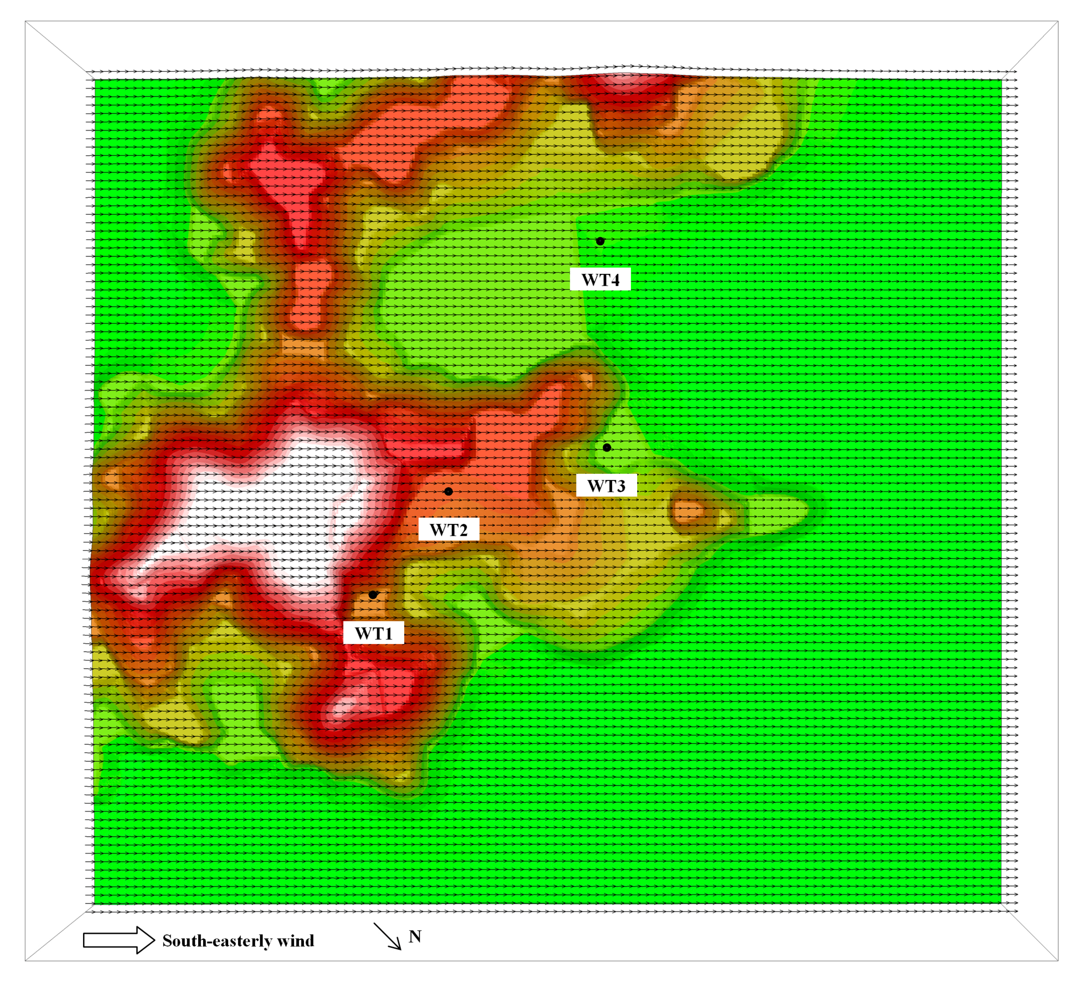
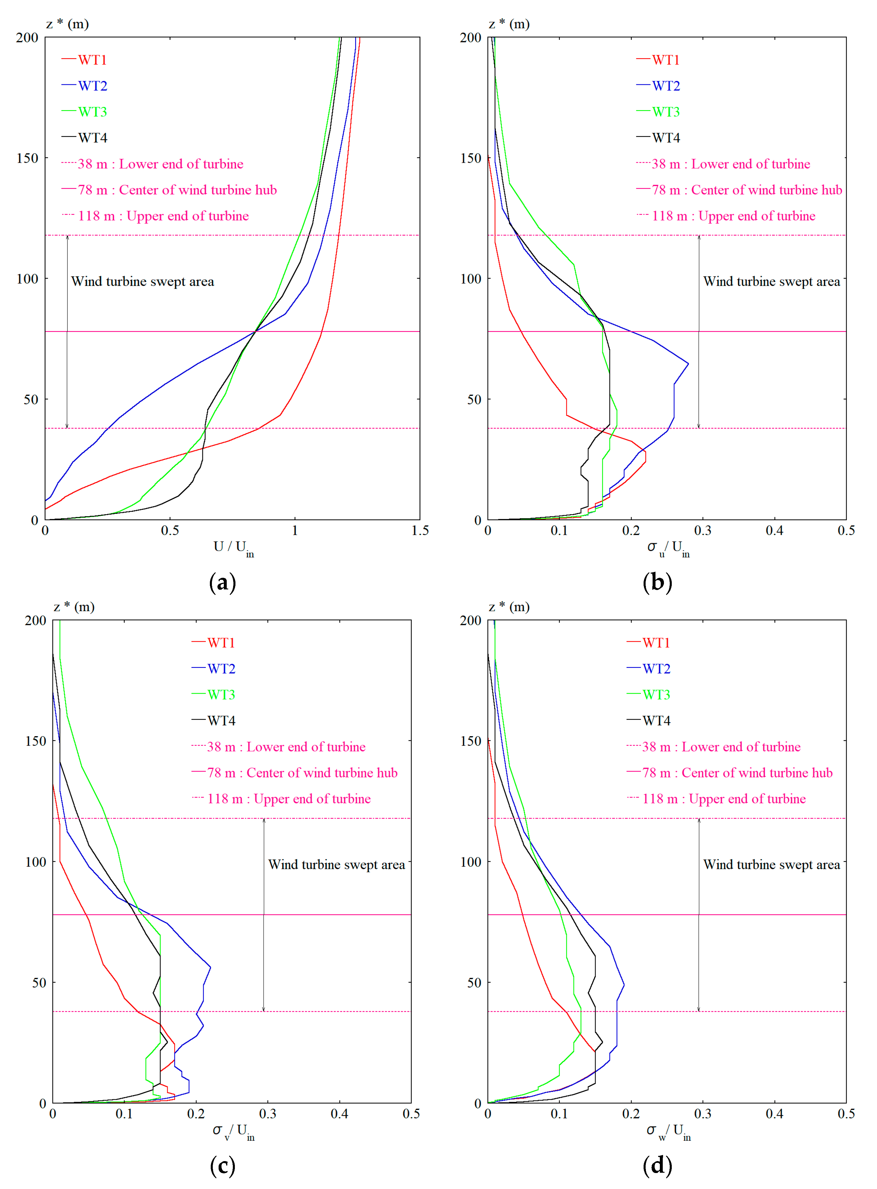
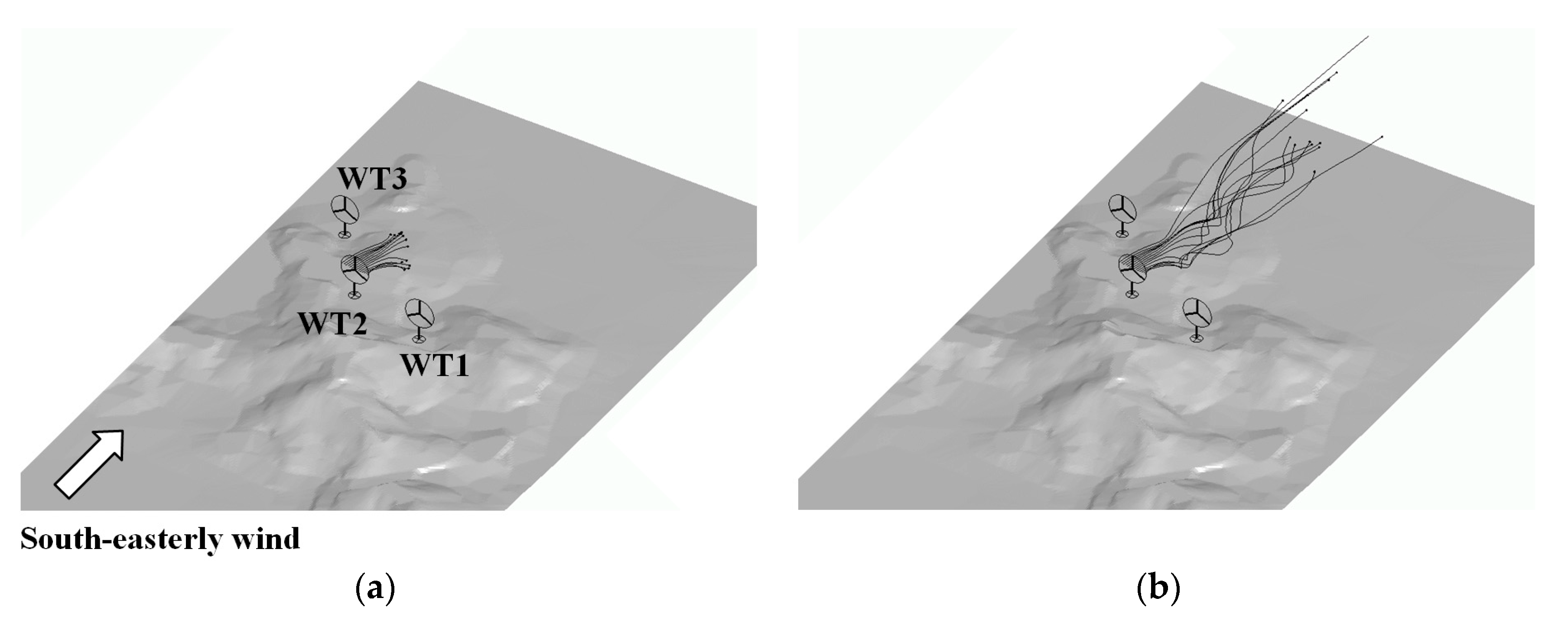
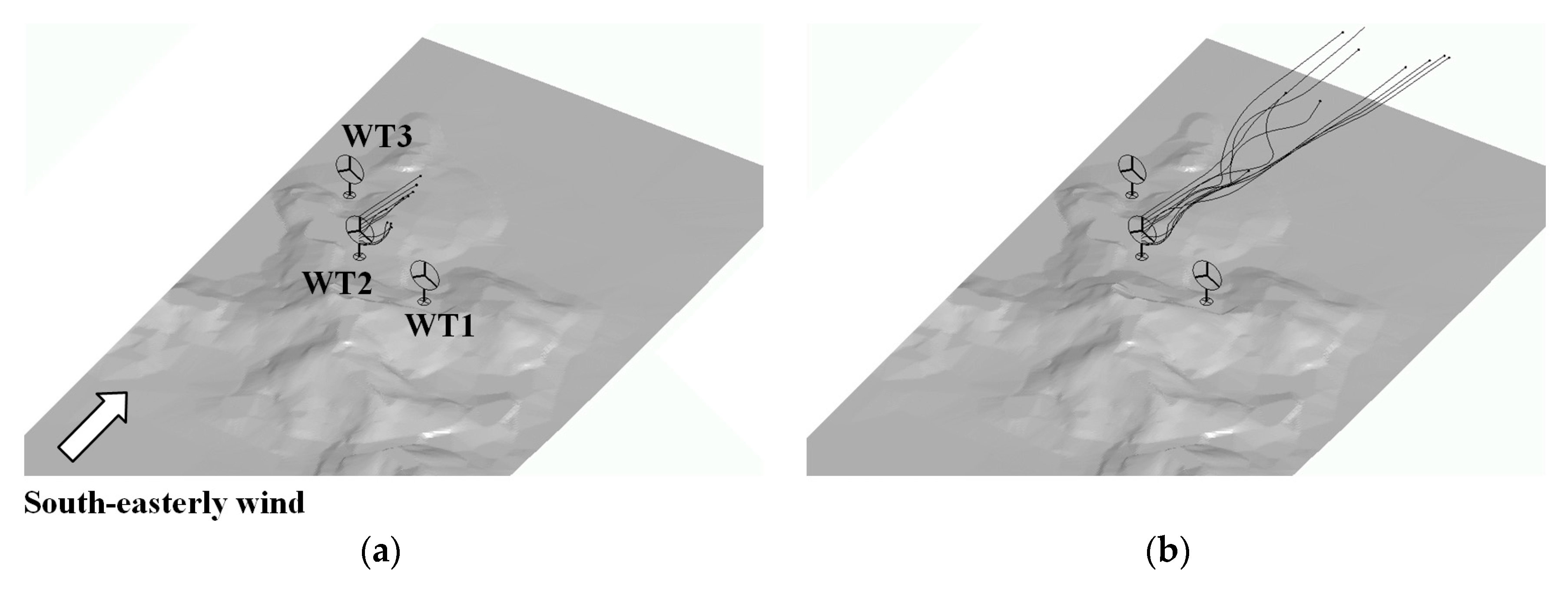
3.3. Simulation Results and Discussions

In the present study, discussions will focus on comparisons between the airflows at WT1 (Wind Turbine 1), which had the best operational performance of all investigated wind turbines, and the airflows at WT2 (Wind Turbine 2), which is presumed to be affected significantly by terrain-induced turbulence in the case of south-easterly wind. (Wind Turbine 1—Wind Turbine 2 will be abbreviated as WT1—WT2, hereafter).
Figure 8 shows the wind velocity vectors at the hub height of the wind turbines (78 m above the ground surface). Specifically, the wind velocity vectors are those from the time-averaged wind field. The time interval used for averaging is 100 to 200 in non-dimensional time. Figure 9 shows wind velocity vectors at both of the investigated wind turbine locations from the same time period used for Figure 8 and Figure 10. The results in Figure 8 and Figure 9 are equivalent to those that would be found by a Reynolds-averaged modeling (RANS). An examination of both results reveals that there exist neither significant wind velocity fluctuations, indicating the presence of terrain-induced turbulence, nor severe deficits in the wind velocity profiles at the locations of the wind turbines. That is, these results would lead to the conclusion that the wind fields at and around the wind turbines are suitable for wind power generation.
However, breakage occurred on the yaw motor and yaw gear of WT2. To accurately simulate the behavior of terrain-induced turbulence, such as that investigated in the present study, the use of the RIAM-COMPACT natural terrain version software, which incorporates a LES model for the unsteady turbulence model, is highly effective. The RIAM-COMPACT software has the ability to output the temporal behaviors of various physical quantities and not just their time-averaged values.
Figure 10 shows the temporal variation of (1) the fluctuating component (deviation from the mean value) of the streamwise (x) wind velocity at the hub height of the wind turbines, and (2) the angle of the wind on horizontal and vertical cross-sections. In the figure, the horizontal axes indicate non-dimensional time. If a wind speed of Uin = 5.0 m/s is assumed, the time in the figure corresponds to approximately 40.0 min. Figure 10 also shows the definitions of the angles of the wind on the horizontal and vertical cross-sections. An inspection of the undulating patterns of the time series in Figure 10 allows a clear understanding of the change in the unsteady wind conditions occurring near the wind turbines.
Subsequently, the fluctuating component (deviation from the mean value) of the streamwise (x) wind velocity will be examined (top panel in Figure 10). In contrast to the very small temporal fluctuations of the streamwise wind velocity at WT1, the presence of spike-like temporal fluctuations can be confirmed at WT2. Although it is beyond the scope of the present paper, further examination of temporal wind velocity changes at the lower, upper, left, and right ends of the swept area allows an examination of the moments exerted on the rotor.
An investigation of the temporal variation in the angle of the wind on the horizontal cross-section (middle panel in Figure 10) reveals the following: As in the case of the wind velocity, the amplitude of the fluctuations of the angle of the wind on the horizontal cross-section is quite small at WT1. On the other hand, changes in the wind direction exceeding 25.0° are frequently seen at WT2 (see also Figure 11). Furthermore, the fact that many spikes occur in the direction of positive values suggests that easterly winds are generated on very short time scales due to the topographic effects.
Finally, the temporal variation in the angle of the wind on the vertical cross-section was examined (bottom panel in Figure 10). This figure also suggests that wind blowing upward and downward, exceeding 25.0° from the horizontal, is generated. It can be speculated that the minor landforms located upwind of the wind turbine contribute to these local wind direction changes.
Figure 11 and Figure 12 illustrate the wind field (wind velocity vectors) from times characterized by the large wind direction changes, indicated by “A” and “B” in Figure 10. An examination of Figure 11 reveals that the direction of the wind aloft at the location of WT2 (easterly wind) deviates significantly from the direction of the prevailing wind. Furthermore, an inspection of Figure 12, which shows the wind field from a different time from that in Figure 11, shows that large upward flow has been generated near the center of the hub of WT2. In addition, the vertical profiles of the streamwise wind velocity in Figure 12 do not follow the so-called wind profile power law; a large velocity deficit can be seen between the hub center and the lower end of the swept area.
In general, the power curve of a wind turbine (the catalog value) is specified using the velocity of the wind flowing into the hub center of the wind turbine on flat terrain, assuming the absence of the turbine itself. Furthermore, the vertical profile of the mean horizontal wind speed, which is used to evaluate the wind shear, is assumed to follow a power law, with a coefficient of approximately 5 to 7. Therefore, a large reduction in the generated electric power is expected in the presence of wind shear, which deviates significantly from the wind shear predicted using the profile based on the power law. Furthermore, such anomalous wind shear will likely be an increasingly important topic of research in the future in connection with the issues of wind turbine tower vibration and the fatigue strength of yaw gears.
Figure 13 shows the vertical profiles of selected physical quantities at each wind turbine location. Figure 13a shows the vertical profile of the mean streamwise wind velocity. Figure 13b–d shows the vertical profiles of the standard deviations of the three wind velocity components. In all these figures, the vertical axes indicate the height above the ground (m), and the horizontal axis is normalized by the inflow wind velocity aloft, Uin). In addition, the vertical range of the wind turbine swept area (the rotor diameter) is also illustrated. In the vertical profile of the mean streamwise wind velocity in Figure 13a, no severe wind velocity deficit is identified at any of the wind turbines, except for WT2. An inspection of the profiles in the vertical range of the wind turbines in Figure 13b–d reveals that the effects of terrain-induced turbulence are almost similar in magnitude at WT3 and WT4, and that, at WT2, it is extremely large due to the presence of the minor landforms upstream of these turbines. The effect of the terrain-induced turbulence is notably smaller at WT1 than at the other three wind turbines.
To assess three-dimensional wind conditions, it is effective to release virtual particles and observe their trajectories (pathlines). Figure 14 and Figure 15 show the results obtained using this method. In Figure 14, virtual particles are released between the right and left edges of the swept area at the height of the center of the wind turbine hub. On the other hand, virtual particles are released between the upper and lower edges of the swept area at the y-coordinate of the center of the wind turbine hub, as shown in Figure 15. As discussed thus far, in the vicinity of WT2, the airflow meanders significantly and three dimensionally in the horizontal and vertical directions due to the effects of the minor landforms located upstream of this wind turbine (Figure 14 and Figure 15).
Finally, it should be recalled that the present study examines only the turbulence generated by the irregularities of the terrain surface and does not take into account the effects of the turbulence caused by gusts.

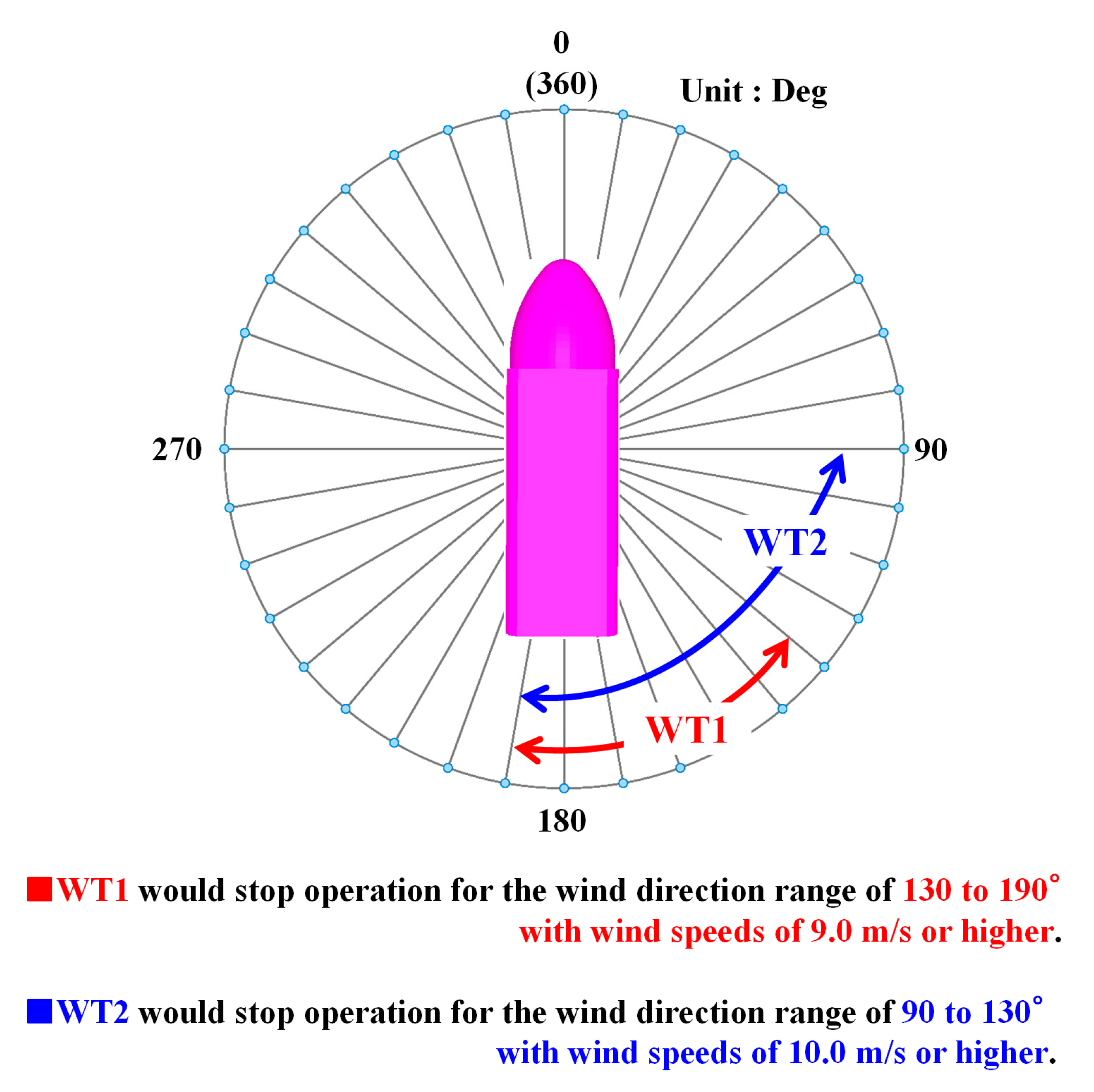
4. The Economic Effects

At the Atsumi Wind Farm in the Aichi Prefecture, Japan (start date of operation: 17 January 2007), the terrain-induced turbulence affected the wind turbines in the form of worn brake pads for yaw motors and fractured planetary gears both due to frequent yaw controls and, also, in the form of hydraulic system failures due to frequent pitch controls.
In the present study, the numerical wind simulation was conducted by reproducing the topography near the wind turbine sites in high resolution and using the Large-Eddy Simulation (LES) technique. The topography near the wind turbine sites serves as the origin of the terrain-induced turbulence. The obtained numerical results showed that the terrain-induced turbulence is generated at a small terrain feature located upstream of WT2 in the case of south-easterly wind. The generated turbulence affects the wind turbine directly. The wind speed and wind direction at the wind turbine site are significantly changed with time.
At the Atsumi Wind Farm, a combination of the series of wind simulation results and on-site operation experience led to a decision to adopt an “automatic shutdown program” for WT1 and WT2 (introduced on 23 May 2011; modified on 26 July 2011). Here, “automatic shutdown program” means the automatic suspension of wind turbine operation based on the wind speed and wind direction meeting the conditions associated with significant effects of terrain-induced turbulence at a wind turbine site. Specifically, after modifications, the program was configured such that WT1 would stop operation for the wind direction range of 130° to 190°, with wind speeds of 9.0 m/s or higher, and that WT2 would stop operation for the wind direction range of 90° to 130°, with wind speeds of 10.0 m/s or higher (see Figure 16). The adoption of the “automatic shutdown program” has successfully led to a large reduction in the number of occurrences of wind turbine damage, in addition to, creating positive economic effects. To evaluate the economic effects, the performance of the wind turbines from the two years preceding the adoption of the “automatic shutdown program” was used as a reference and changes in the capacity and availability factors were calculated from the reduction in downtime of the wind turbines from the two years following the adoption of the “automatic shutdown program.” The following major economic effects have been realized based on converting the performance of the two wind turbines combined from the two years preceding and the two years following the adoption of the “automatic shutdown program” into the performance of a single wind turbine per year:
(1)
A reduction in the repair costs by 9.322 million yen per year per wind turbine,
(2)
An increase in the availability factor by 8.05% (87.3%→95.4%), and
(3)
An increase in the capacity factor by 1.7% (21.2%→22.9%).
The number of occurrences of damage to wind turbines can be reduced significantly by combining suitability inspections of local wind conditions” by RIAM-COMPACT, that is, numerical wind simulations (analyses of terrain-induced turbulence), with appropriate wind turbine control based on the results of the diagnoses. At the same time, this combination of approaches also results in significant positive economic effects. In the future development of the wind power industry in Japan, it is essential to adopt suitability inspections of local wind conditions” for each of the country’s land-based wind turbines.

5. Conclusions

The wind conditions at the Atsumi Wind Farm in the Aichi Prefecture, Japan (in operation since March 2007) were numerically predicted using the RIAM-COMPACT natural terrain version software. The simulation results showed that the minor landforms located upstream of WT2 serve as the origin of turbulence (terrain-induced turbulence), in the case of south-easterly wind, and that WT2 is strongly affected by this turbulence.
The use of time-averaged RANS turbulence models creates severe difficulties in simulating the effects of terrain-induced turbulence generated locally due to minor landforms and small topographical irregularities distributed sparsely around wind turbines. As a result, the use of RANS models tends to miss the presence of such effects. Therefore, it is effective to adopt an approach based on an unsteady turbulence model (e.g., LES), such as the RIAM-COMPACT.
In addition, relative comparisons of the effects of terrain-induced turbulence among wind turbines, such as that presented in the present study, can be made appropriately using only detailed terrain data accurately representing the land formations at a site of interest, without the use of any meteorological data. If the results from such comparisons were to be effectively applied to wind turbine operation control, the number of internal and external breakdowns of wind turbines caused by terrain-induced turbulence would decrease dramatically, which would likely allow the availability factors of wind turbines to increase significantly. For example, meteorological conditions in which large wind direction and speed changes occur so rapidly that they cannot be adequately counteracted by the pitch angle control of the wind turbine blades (i.e., specific wind directions in which such meteorological conditions occur) can be predicted in advance for the position of each nacelle. When the actual meteorological conditions meet the previously identified meteorological conditions, measures, such as halting wind power generation, can be taken.
In the future, regardless of whether the terrain is flat or complex, it is necessary (1) to conduct a detailed wind synopsis diagnosis, such as the one presented in this paper, for all wind directions around a wind turbine; (2) to accurately understand the three-dimensional local wind conditions at each wind turbine location and the temporal change of the vertical profiles of the wind velocities at wind turbine locations; and (3) to carefully consider the wave-like structures in the time series of the wind velocities and the turbulence intensities at the lower, upper, left, and right ends of the swept area.

Acknowledgments

For conducting this research, the author was provided with the various types of data on the Atsumi Wind Farm, Aichi Prefecture, Japan by Kyudenko New Energy Co., Ltd. For the analyses based on the above-mentioned data, the author was received cooperation from West Japan Engineering Consultants, Inc. In addition, this research was supported by JSPS KAKENHI Grant Number 17H02053. The author would like to express his gratitude to all the organizations.

Conflicts of Interest

The authors declare no conflict of interest.

References

  1. Palma, J.M.L.M.; Castro, F.A.; Ribeiro, L.F.; Rodrigues, A.H.; Pinto, A.P. Linear and nonlinear models in wind resource assessment and wind turbine micro-siting in complex terrain. J. Wind Eng. Ind. Aerodyn. 2008, 96, 2308–2326. [Google Scholar] [CrossRef] [Green Version]
  2. Prospathopoulos, J.M.; Politis, E.S.; Chaviaropoulos, P.K. Application of a 3D RANS solver on the complex hill of Bolund and assessment of the wind flow predictions. J. Wind Eng. Ind. Aerodyn. 2012, 107–108, 149–159. [Google Scholar] [CrossRef]
  3. Diebold, M.; Higgins, C.; Fang, J.; Bechmann, A.; Parlange, M.B. Flow over hills: A large-eddy simulation of the Bolund case. Bound.-Layer Meteorol. 2013, 148, 177–194. [Google Scholar] [CrossRef]
  4. Conan, B.; Chaudhari, A.; Aubrun, S.; van Beeck, J.; Hämäläinen, J.; Hellsten, A. Experimental and numerical modelling of flow over complex terrain: The Bolund hill. Bound.-Layer Meteorol. 2016, 158, 183–208. [Google Scholar] [CrossRef]
  5. Sessarego, M.; Shen, W.Z.; van der Laan, M.P.; Hansen, K.S.; Zhu, W.J. CFD Simulations of Flows in a Wind Farm in Complex Terrain and Comparisons to Measurements. Appl. Sci. 2018, 8, 788. [Google Scholar] [CrossRef]
  6. Astolfi, D.; Castellani, F.; Terzi, L. A Study of Wind Turbine Wakes in Complex Terrain Through RANS Simulation and SCADA Data. J. Sol. Energy Eng. 2018, 140, 031001. [Google Scholar] [CrossRef]
  7. Uchida, T.; Ohya, Y. Verification of the Prediction Accuracy of Annual Energy Output at Noma Wind Park by the Non-Stationary and Non-Linear Wind Synopsis Simulator, RIAM-COMPACT. J. Fluid Sci. Technol. 2008, 3, 344–358. [Google Scholar] [CrossRef]
  8. Uchida, T.; Ohya, Y. Latest Developments in Numerical Wind Synopsis Prediction Using the RIAM-COMPACT CFD Model-Design Wind Speed Evaluation and Wind Risk (Terrain-Induced Turbulence) Diagnostics in Japan. Energies 2011, 4, 458–474. [Google Scholar] [CrossRef]
  9. Watanabe, F.; Uchida, T. Micro-siting of Wind Turbine in Complex Terrain: Simplified Fatigue Life Prediction of Main Bearing in Direct Drive Wind Turbines. Wind Eng. 2015, 39, 349–368. [Google Scholar] [CrossRef]
  10. Uchida, T. High-Resolution LES of Terrain-Induced Turbulence around Wind Turbine Generators by Using Turbulent Inflow Boundary Conditions. Open J. Fluid Dyn. 2017, 7, 511–524. [Google Scholar] [CrossRef]
  11. Uchida, T. High-Resolution Micro-Siting Technique for Large Scale Wind Farm Outside of Japan Using LES Turbulence Model. Energy Power Eng. 2017, 9, 802–813. [Google Scholar] [CrossRef]
  12. Takanori Uchida, T. CFD Prediction of the Airflow at a Large-Scale Wind Farm above a Steep, Three-Dimensional Escarpment. Energy Power Eng. 2017, 9, 829–842. [Google Scholar] [CrossRef]
  13. Kawashima, Y.; Uchida, T. Effects of Terrain-Induced Turbulence on Wind Turbine Blade Fatigue Loads. Energy Power Eng. 2017, 9, 843–857. [Google Scholar] [CrossRef]
  14. Uchida, T. Large-Eddy Simulation and Wind Tunnel Experiment of Airflow over Bolund Hill. Open J. Fluid Dyn. 2018, 8, 30–43. [Google Scholar] [CrossRef]
  15. Uchida, T. Computational Fluid Dynamics (CFD) Investigation of Wind Turbine Nacelle Separation Accident over Complex Terrain in Japan. Energies 2018, 11, 1485. [Google Scholar] [CrossRef]
  16. Kim, J.; Moin, P. Application of a fractional-step method to incompressible Navier-Stokes equations. J. Comput. Phys. 1985, 59, 308–323. [Google Scholar] [CrossRef]
  17. Kajishima, T. Upstream-shifted interpolation method for numerical simulation of incompressible flows. Trans. Japan Soc. Mech. Eng. B 1994, 60, 3319–3326. (In Japanese) [Google Scholar] [CrossRef]
  18. Kawamura, T.; Takami, H.; Kuwahara, K. Computation of high Reynolds number flow around a circular cylinder with surface roughness. Fluid Dyn. Res. 1986, 1, 145–162. [Google Scholar] [CrossRef]
  19. Smagorinsky, J. General circulation experiments with the primitive equations. Part 1, Basic experiments. Mon. Weather Rev. 1963, 91, 99–164. [Google Scholar] [CrossRef]
Figure 1. Terrain at and in the vicinity of the Atsumi wind farm, Aichi Prefecture, Japan.
Energies 11 01530 g001
Figure 2. A photo of the wind turbine site (taken by one of the authors from the north-west). Note: Minor landforms of 125 m in elevation can be seen behind WT2 (Wind Turbine 2).
Energies 11 01530 g002
Figure 3. A photo of WT1 (Wind Turbine 1) showing specifications of the wind turbines.
Energies 11 01530 g003
Figure 4. Computational domain, bird’s eye view, colors indicate the elevation.
Energies 11 01530 g004
Figure 5. Computational grid cells.
Energies 11 01530 g005
Figure 6. Non-dimensional inflow profile.
Energies 11 01530 g006
Figure 7. Characteristic two scales used in the present simulation.
Energies 11 01530 g007
Figure 8. Wind velocity vectors at the wind turbine hub-height (78 m), time-averaged field. The averaging time period is 100 to 200 in non-dimensional time (see Figure 10).
Energies 11 01530 g008
Figure 9. Wind velocity vectors at the wind turbine locations, time-averaged field. The averaging time period is 100 to 200 in non-dimensional time (see Figure 10).
Energies 11 01530 g009
Figure 10. Fluctuating streamwise (x) component of the wind at the hub-height of the wind turbines (Figure 10a). Temporal change in the angle of the wind on the horizontal (Figure 10b) and vertical (Figure 10c) cross-sections at the hub-height of the wind turbines. Figure 10d also shows the definitions of the angles of the wind on the horizontal and vertical cross-sections. With an assumed wind speed of Uin = 5.0 m/s, the time period on the horizontal axes is equivalent to approximately 40.0 min
Energies 11 01530 g010
Figure 11. Wind velocity vectors at the wind turbine hub-height (78 m). Instantaneous field from the time indicated by “A” in Figure 10.
Energies 11 01530 g011
Figure 12. Wind velocity vectors at the wind turbine locations. Instantaneous field from the time indicated by “B” in Figure 10.
Energies 11 01530 g012
Figure 13. Vertical profiles of various physical quantities at the wind turbine locations. (a) Profiles of mean streamwise wind velocity (b) Standard deviation of the streamwise wind velocity (c) Standard deviation of the spanwise wind velocity (d) Standard deviation of the vertical wind velocity.
Energies 11 01530 g013
Figure 14. Trajectories (pathlines) of virtual particles released from the location of WT2. Virtual particles are released at the height of the center of the wind turbine hub, across a straight line between the left and right ends of the swept area. (a) At non-dimensional time, t. (b) At non-dimensional time, t + Δt.
Energies 11 01530 g014
Figure 15. Trajectories (pathlines) of virtual particles released from the location of WT2. Virtual particles are released at the y-coordinate of the center of the wind turbine hub, across a straight line between the lower and upper ends of the swept area. (a) At non-dimensional time, t. (b) At non-dimensional time, t + Δt.
Energies 11 01530 g015
Figure 16. Conceptual diagram of “automatic shutdown program” for WT1 and WT2.
Energies 11 01530 g016
Table 1. Summary of the Atsumi Wind Farm.
WT1 to WT4
Wind turbine manufacturer, outputVestas Wind Systems A/S V80-2.0 MW
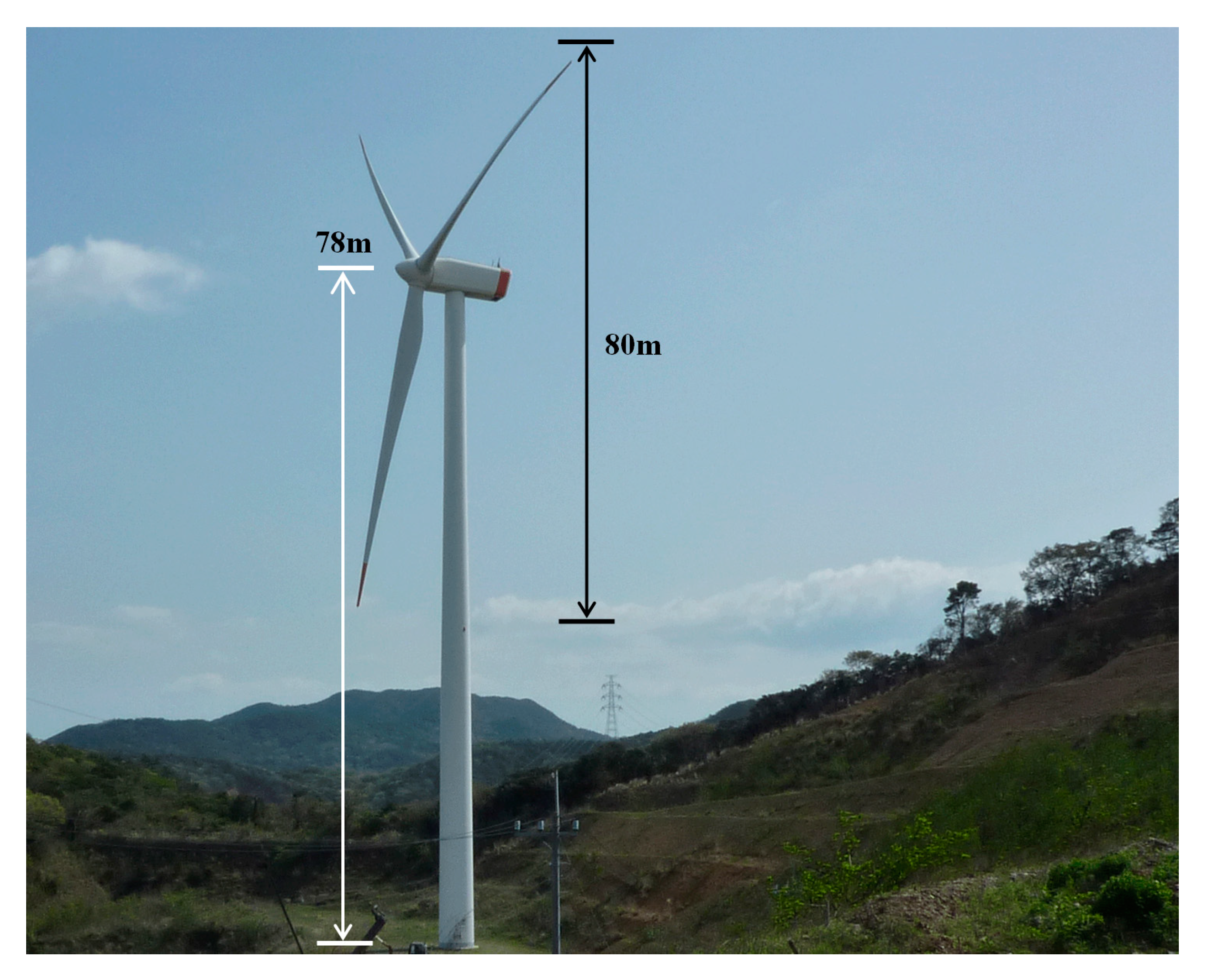
Wind turbine height (ground surface to hub center height)78 m
Blade diameter80 m

