A Distributed PV System Capacity Estimation Approach Based on Support Vector Machine with Customer Net Load Curve Features

Abstract

Most distributed photovoltaic systems (DPVSs) are normally located behind the meter and are thus invisible to utilities and retailers. The accurate information of the DPVS capacity is very helpful in many aspects. Unfortunately, the capacity information obtained by the existing methods is usually inaccurate due to various reasons, e.g., the existence of unauthorized installations. A two-stage DPVS capacity estimation approach based on support vector machine with customer net load curve features is proposed in this paper. First, several features describing the discrepancy of net load curves between customers with DPVSs and those without are extracted based on the weather status driven characteristic of DPVS output power. A one-class support vector classification (SVC) based DPVS detection (DPVSD) model with the input features extracted above is then established to determine whether a customer has a DPVS or not. Second, a bootstrap-support vector regression (SVR) based DPVS capacity estimation (DPVSCE) model with the input features describing the difference of daily total PV power generation between DPVSs with different capacities is proposed to further estimate the specific capacity of the detected DPVS. A case study using a realistic dataset consisting of 183 residential customers in Austin (TX, U.S.A.) verifies the effectiveness of the proposed approach.

1. Introduction

1.1. Background and Motivation

Grid-connected distributed photovoltaic system (DPVS) is playing an increasingly significant role as an electric supply resource. The worldwide rooftop photovoltaic (PV) installations reached nearly 40 GW by the end of 2017, which is twice as much as in 2016 [1]. It is estimated by the International Energy Agency (IEA) that the total distributed PV capacity installed in 2016 in the U.S., Germany, Sweden, Spain and China is 4169 MW, 1225 MW, 70.7 MW, 36.1 MW and 4230 MW, respectively [2]. Particularly, the growth of DPVS installations in China is predicted to be 20 GW per year from 2017 to 2020.

Introducing a high penetration of DPVSs to the grid could have significant impacts on many aspects, including demand response (DR) capacity estimation [3,4,5,6], customer baseline load estimation [7,8], load forecasting [9,10] and distribution network planning [11,12]. Specifically, in terms of DR capacity estimation, the DR aggregators need to estimate how much DR capacity they have in order to formulate the reasonable bidding strategy in the electricity market. The DR capacity is highly related to the load profiles. The DPVS installations will significantly affect the load profiles and thereby affect the available DR capacity. Large errors will occur in DR capacity estimation if the latest DPVS capacity information is unknown. Similarly, a lack of knowledge about the installed DPVSs will also lead to biased baseline load estimation results, high errors in load forecasting and improper network planning.

Generally, most DPVSs are normally located behind meters, and their real online operating capacity cannot be easily obtained from existing measurements. Hence, there is a growing need among utilities, retailers and third party companies (e.g., DR aggregators) to obtain such high quality capacity information. However, the existing methods for collecting the capacity information such as original installation records or surveys are usually incomplete, costly and time consuming [13]. What’s more, the information obtained by the existing methods is usually inaccurate due to the following reasons: (1) the existence of unauthorized DPVS. For example, a large number of unauthorized DPVSs were recognized by Hawaii Electric Company in 2014 [14]. These unauthorized DPVSs have no installation records; (2) DPVS capacity expansion without permission applications; (3) DPVSs that have totally or partly stopped running due to faults. These unauthorized, expanded and faulty DPVSs are invisible from the measurements and thus it is difficult to obtain the accurate capacity information by the existing methods. Therefore, it is essential to explore new methods to realize reliable and accurate DPVS capacity estimation (DPVSCE).

1.2. Literature Review

The research on DPVSCE has recently started to receive attention in the past few years. To date, very few papers have attempted to estimate the capacity of each individual DPVS. Malof et al. presented an object detection algorithm for automatically identifying the location and size of small-scale solar PV arrays using high-resolution color satellite imagery [15]. This work demonstrates the feasibility of collecting distributed PV information over large areas using aerial or satellite imagery, however, some limitations can be observed. First, manual annotations of true rooftop PV locations are needed in this method for training and validating, which is time-consuming. Second, it is not easy to obtain such latest high-resolution (≤0.3 km) color satellite imagery in reality. More importantly, this method only can roughly estimate the physical size of PV arrays but is unable to estimate the specific capacity because the capacity of PV arrays of the same size of could be different.

Zhang et al. proposed a data-driven approach for the detection, verification, and estimation of residential PV systems based on smart meter data [16]. The authors first adopted a change-point detection algorithm to identify the potential unauthorized PV installations and then used a statistical inference to further verify them. Finally, local cloud cover index was integrated with smart meter data to estimate the capacity of PV system. This method is effective under an impractical assumption that only when the characteristics of all other loads before and after unauthorized PV installations are almost unchanged. This method needs the load data before and after PV installations, which make it unable to work if the load data is unavailable before installations.

1.3. Contributions

In order to address the above problems, a two-stage DPVS capacity estimation approach based on support vector machine (SVM) with customer net load curve features is proposed in this paper. The main contributions of this paper are summarized as follows:

• A one-class support vector classification (SVC)-based DPVS detection (DPVSD) model with the input features extracted according to the unique weather status driven characteristic of DPVS output power is proposed to distinguish customers with DPVSs from those without. This model can not only accurately detect the existence of DPVS, but also reliably distinguish load components showing similar output characteristic to DPVS, such as electric vehicles and energy storage devices, which means it is robust to the interference from those load components that are most likely misrecognized by other methods.
• A bootstrap-support vector regression (SVR) based DPVSCE model with the input features describing the difference of daily total PV power generation between DPVSs with different capacities is proposed to further estimate the specific capacity of the detected DPVS. This model can keep stable promising performance under the scenario of limited training samples and imbalance dataset.
• The effectiveness of the proposed approach is verified on a realistic dataset. Furthermore, the robustness of the model under several scenarios (e.g., the existence of storage devices, different lengths of available historical data) is analyzed and discussed.

1.4. Structure of This Paper

The rest of the paper is organized as follows: Section 2 illustrates the problem formulation and presents the framework of the proposed method. In Section 3, a one-class SVC-based DPVSD model is presented. In Section 4, a bootstrap-SVR-based DPVSCE model is proposed to further estimate the capacities for those detected DPVSs. In Section 5, a case study is presented to verify the effectiveness of the proposed approach. Section 6 tests the robustness of the proposed approach under different scenarios. Section 7 highlights the concluding remarks and further works in future.

2. Problem Formulation

2.1. Problem Statement

Assume the smart meter collects the historical electricity load consumption data for several days, denoted by a set $\mathit{D}$, $\mathit{D}=\{d|d=1,2,\dots ,D\}$. For a certain day, it can be divided into several timeslots, denoted by $\mathit{T}=\{t|t=1,2,\dots ,T\}$. The net load power on day $d$ at timeslot $t$ can be expressed using Equation (1):

$$P_{net}(d,t)=P_{use}(d,t)-P_{pv}(d,t),d\in \mathit{D},t\in \mathit{T}$$

(1)

where $P_{use}(d,t)$ and $P_{pv}(d,t)$ are the actual load power and PV output power on day d at timeslot t. For those customers without DPVSs, the PV output power is equal to 0, i.e., $P_{pv}(d,t)=0\forall d\in \mathit{D},t\in \mathit{T}$.

For those authorized customers, utilities usually know the detailed information about their DPVSs, including the capacity, location and installation date, etc. The aim of this paper is to detect whether other customers have installed DPVSs or not and further estimate their capacities, which can be formulated as a supervised learning problem.

2.2. Framework of the Proposed Approach

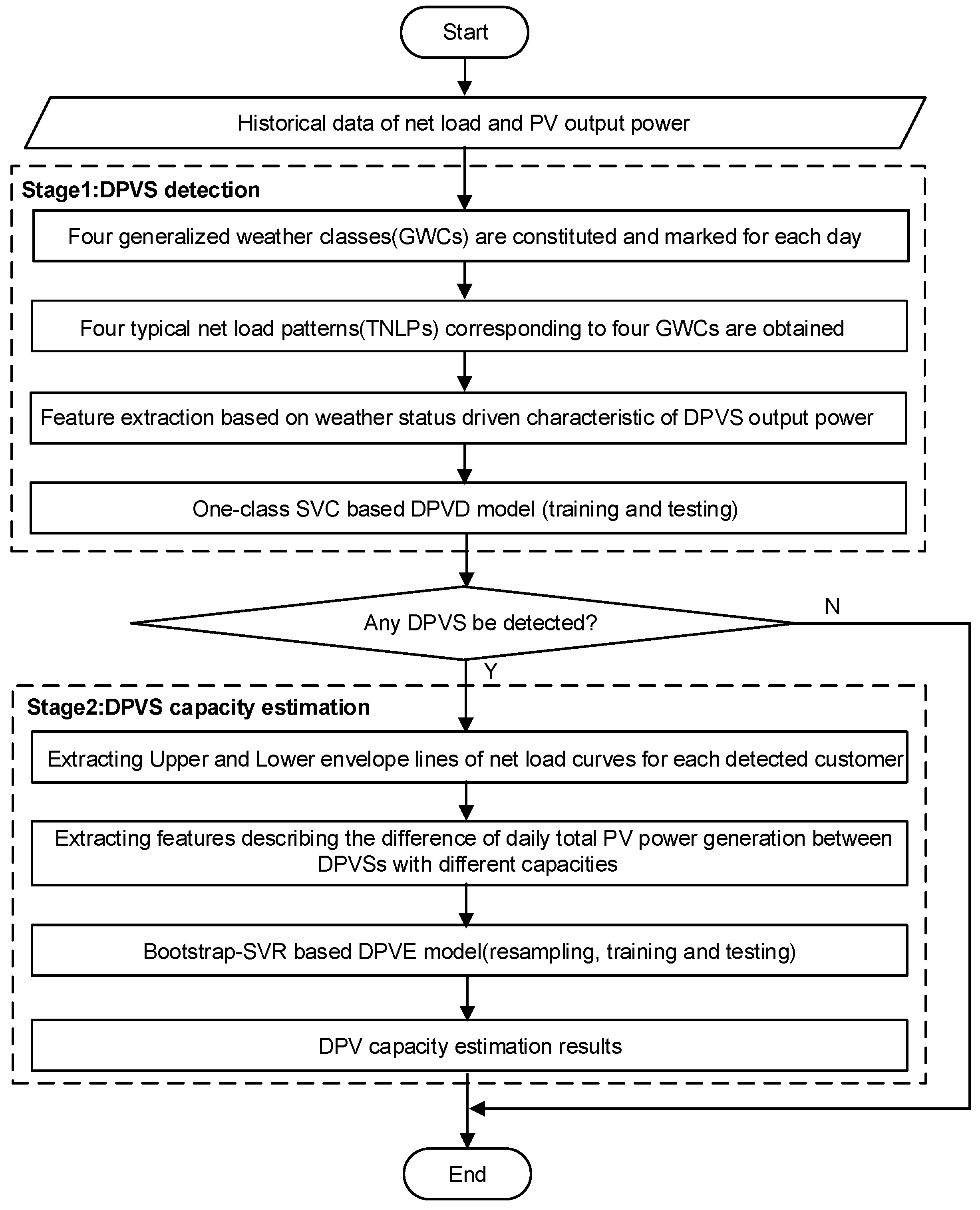
Due to the possible interference from other load components that exhibit similar output characteristics like DPVS, such as electric vehicles and energy storage systems, it is difficult to directly estimate the capacity of DPVS. Hence, the proposed DPVSCE approach has been split into two stages named detection and estimation. The framework of the proposed approach is shown in Figure 1 and the details are illustrated in the following sections.

3. One-Class SVC Based DPVSD Model

The significant distinction between DPVS and other load components is that the output power DPVS is weather status driven while other load components are not. In this section, several features utilizing this distinction are extracted to distinguish the DPVS from other load components. Then a one-class SVC model with the extracted features will be used to determine whether a customer has a DPVS or not.

3.1. Generalized Weather Classes

To depict the weather status driven characteristic of DPVS output power, the first step is to perform weather status classification. Four generalized weather classes (GWCs), denoted by GWC-A, B, C, D, covering all weather types were described in our previous work [17]. Different GWCs correspond to different PV output power levels. Historical weather type data is usually needed for generating the GWC labels for each day to show which GWC it belongs to. In order to make the proposed approach be independent of any external weather type data resource, a voting-based GWC label generating method is designed using the actual PV output power data of some customers whose output power is known. The flow chart of the GWC label generating method is shown in Figure 2. Joining K-means clustering and voting method generate a GWC label for each day. It should be noted that multiple rather than single customer’s PV output data has been used to determine the specific GWC label for each day so as to make the final results more reliable. As such, the GWC label of each day can be obtained. Then the set $\mathit{D}$ can be divided into four subsets named ${\mathit{D}}_A,{\mathit{D}}_B,{\mathit{D}}_C,{\mathit{D}}_D$ according to the GWC label. Each subset contains all days belonging to the corresponding GWC.

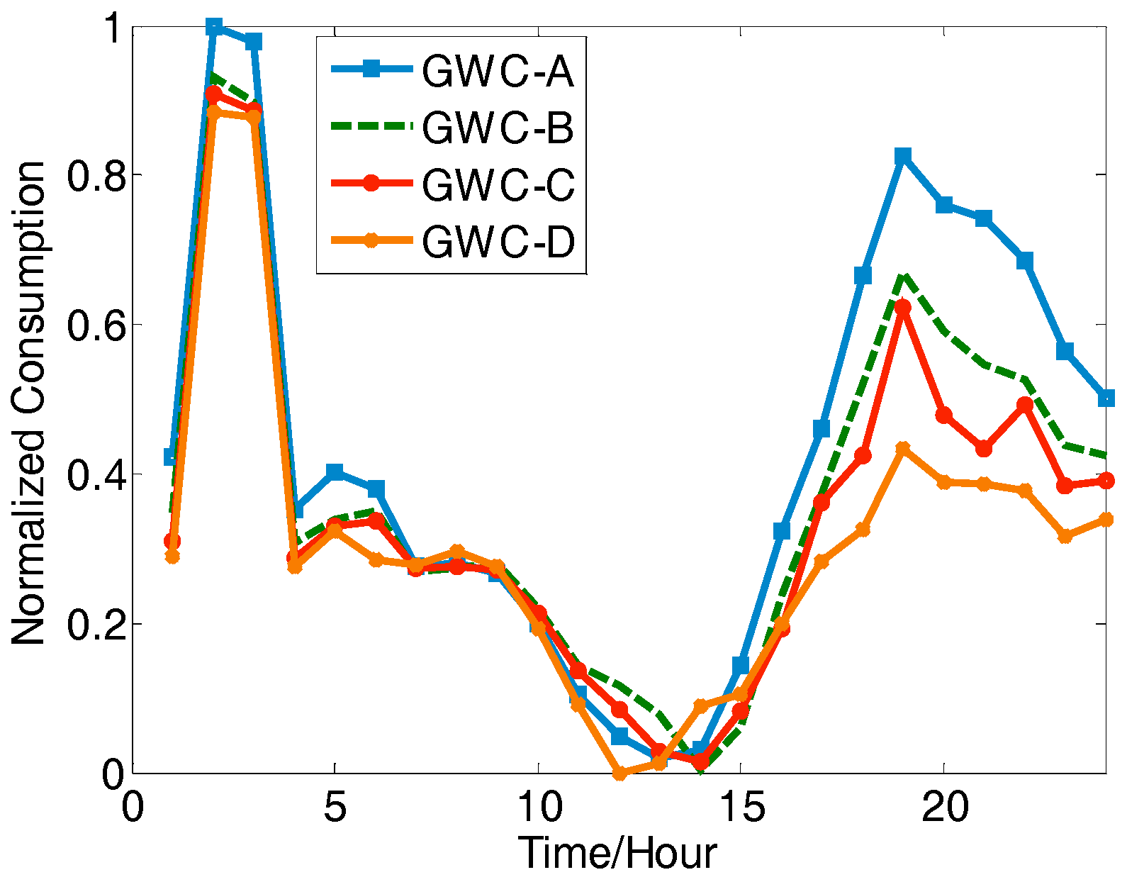
3.2. Typical Net Load Pattern

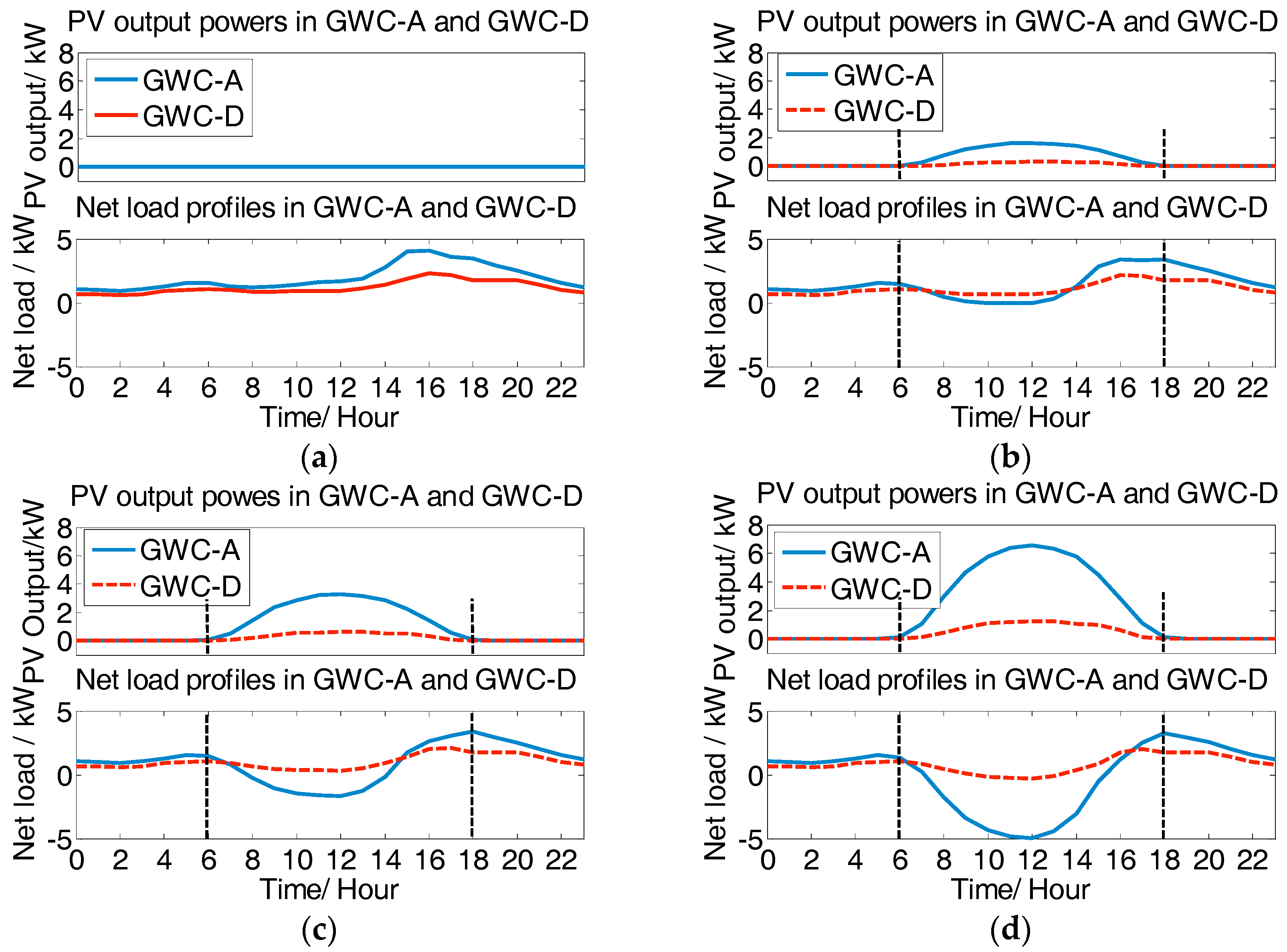
The installation of DPVS will reshape customers’ net load profiles. As shown in Figure 3, the net load profiles in GWC-A and GWC-D show different shapes. This difference becomes more and more obvious with the increase of PV capacity, which means that the net load profile contains abundant information about whether the customer has an operating DPVS or not and the specific PV capacity. Hence, it can be utilized to perform the DPVS detection and estimation.

The main difficulty of using net loads to detect DPVSs is that the other load components will also affect a customer’s net load shape. Compared with industrial and commercial customers, residential customers show more variable load patterns due to their random electricity consumption behaviors. To mitigate the negative impact of the variability of daily load profiles on the detection and reveal the typical consumption behaviors of customers, four typical net load patterns (TNLPs) of each customer in four GWCs are extracted by averaging the daily load profiles in the same GWC, given by Equation (2).

$$TNL{P}^{D_w}(t)=\frac{1}{\left|D_w\right|}{\displaystyle \sum _{d\in D_w}{P}_{net}(d,t)},w\in \{A,B,C,D\}$$

(2)

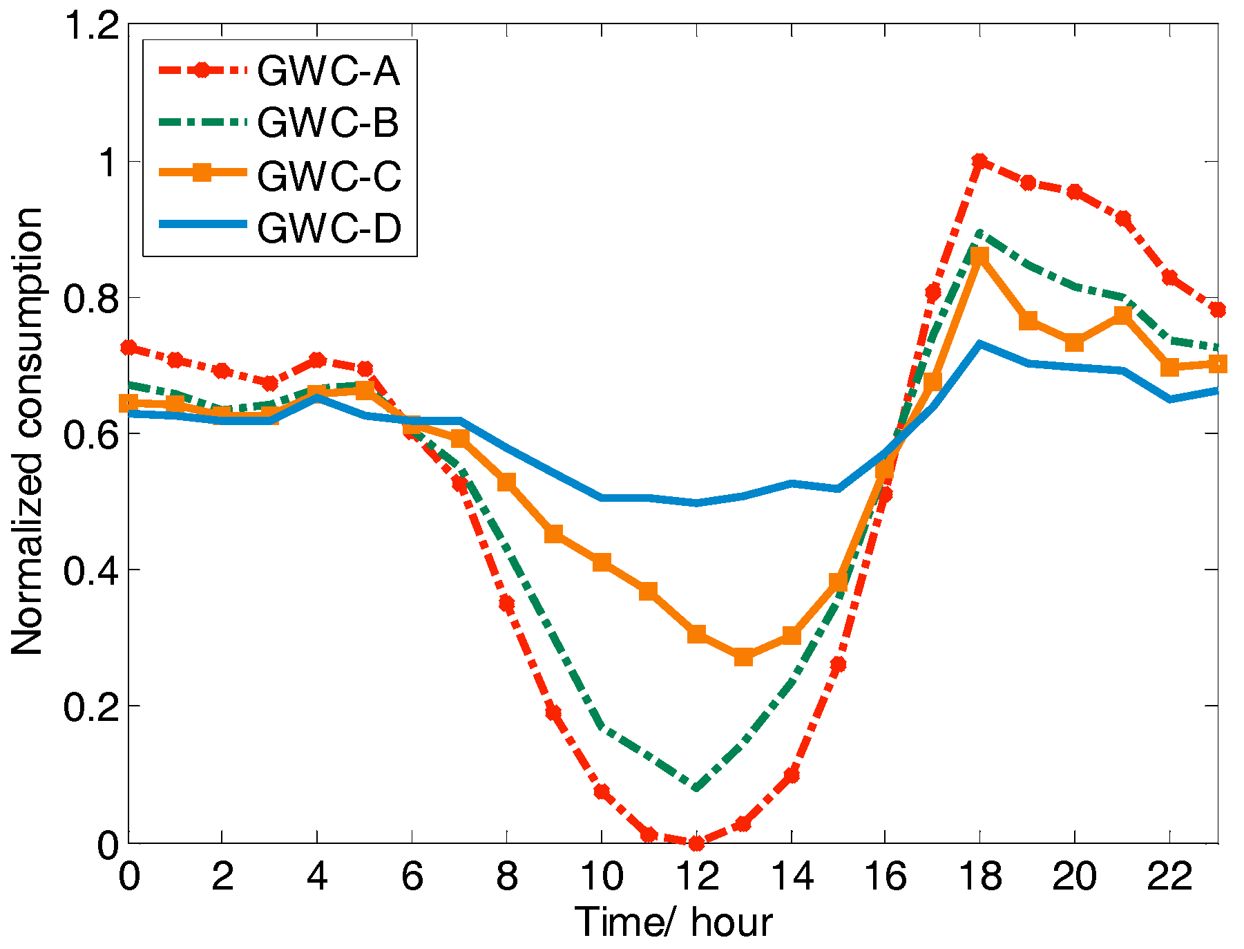
where $\left|D_w\right|$ represents the number of elements in set $D_w$. An example of TNLPs in different GWCs is shown in Figure 4. Then several features will be extracted from these TNLPs in the next section.

3.3. Feature Extraction

As one of the important steps, feature extraction has a large impact on the performance of machine learning methods [18,19]. Suitable features should be able to distinguish between the customers with DPVSs from those who don’t have. It is noted that the TNLPs of customers with DPVSs are considerably different in different GWCs, while these TNLPS are similar for those customers without DPVSs. This is because the output power of DPVSs is weather status driven, while other load components are not. This unique characteristic makes it possible to detect the DPVSs using net load data. Therefore, analysis of the difference between TNLPs in different GWCs is the key point for extracting suitable features.

To further mitigate the negative influence of load pattern variation on the detection, attention is paid to the time period in which the solar power generation is obvious. Hence, we select a time window $\mathbf{\delta }=[t_s,t_e]$ and use the TNLP segment $TNLP(\mathbf{\delta })$ to extract features instead of using the whole TNLP (the time window is set to be 9:00 to 16:00 in this paper). Four weather status-driven features describing the discrepancy between customers with DPVSs and those who don’t have are extracted as follows.

3.3.1. Ratio of Total Electricity Consumption in GWC-A to GWC-D

The amplitudes of TNLPs in different GWCs are different, this difference is particularly obvious between GWC-A and GWC-D. The first feature, denoted by $F_1$, is the ratio of the absolute value of total consumption during time window in GWC-A to it in GWC-D, which is defined as Equation (3).

$$F_1=\frac{{\displaystyle {\sum }_{t=t_s}^{t=t_e}\left|TNL{P}^A(t)\right|}}{{\displaystyle {\sum }_{t=t_s}^{t=t_e}\left|TNL{P}^D(t)\right|}}$$

(3)

For customers with DPVSs, the value of this feature should be greater or much greater than 1, while for those customers without DPVSs, this index should be close to 1.

3.3.2. Concave Shape Index

The integration of DPVSs will affect the net load shape. Specifically, the net load curve will be concave during time window $\mathbf{\delta }$. This phenomenon is more evident in GWC-A, because the solar PV generation is much larger in this GWC compared with other GWCs. Thus, the second feature named concave shape index denoted by $F_2$ is extracted based on the TNLP in GWC-A, namely $TNL{P}^A$.

Once the time window $\mathbf{\delta }$ is determined, there exists a line $\mathit{l}$ connecting the start point and the end point. And the linear equation of this line $\mathit{l}$ can be described by Equation (4):

$$y(t)=TNL{P}^A(t_s)+(t-t_s)\ast \frac{TNL{P}^A(t_e)-TNL{P}^A(t_s)}{t_e-t_s}$$

(4)

where $y(t)$ represents the sampling point on this line $\mathit{l}$ at timeslot t. All of these sampling points form a set, named $\mathit{S}$ and $\mathit{S}=\{y(t)|t\in [t_s,t_e]\}$.The TNLP sampling points below the line $\mathit{l}$ can be expressed as Equation (5):

$${\mathit{S}}^{-}=\{TNL{P}^A(t)|t\in [t_s,t_e],TNL{P}^A(t)<y(t)\}$$

(5)

Then the concavo shape index can be calculated by Equation (6):

$$F_2=\mathrm{card}({\mathit{S}}^{-})/\mathrm{card}(\mathit{S})$$

(6)

where $\mathrm{card}(·)$ represents the counts of elements in a set. This feature describes the proportion of the sampling points below the line $\mathit{l}$, which can be used to characterize the concavity of the TNLP curve during time window $\mathbf{\delta }$.

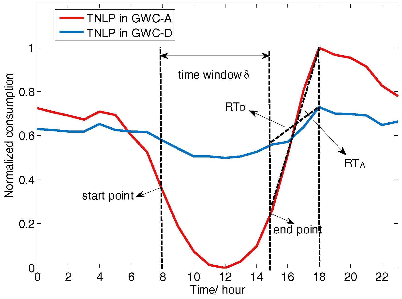
3.3.3. Concavity Degree

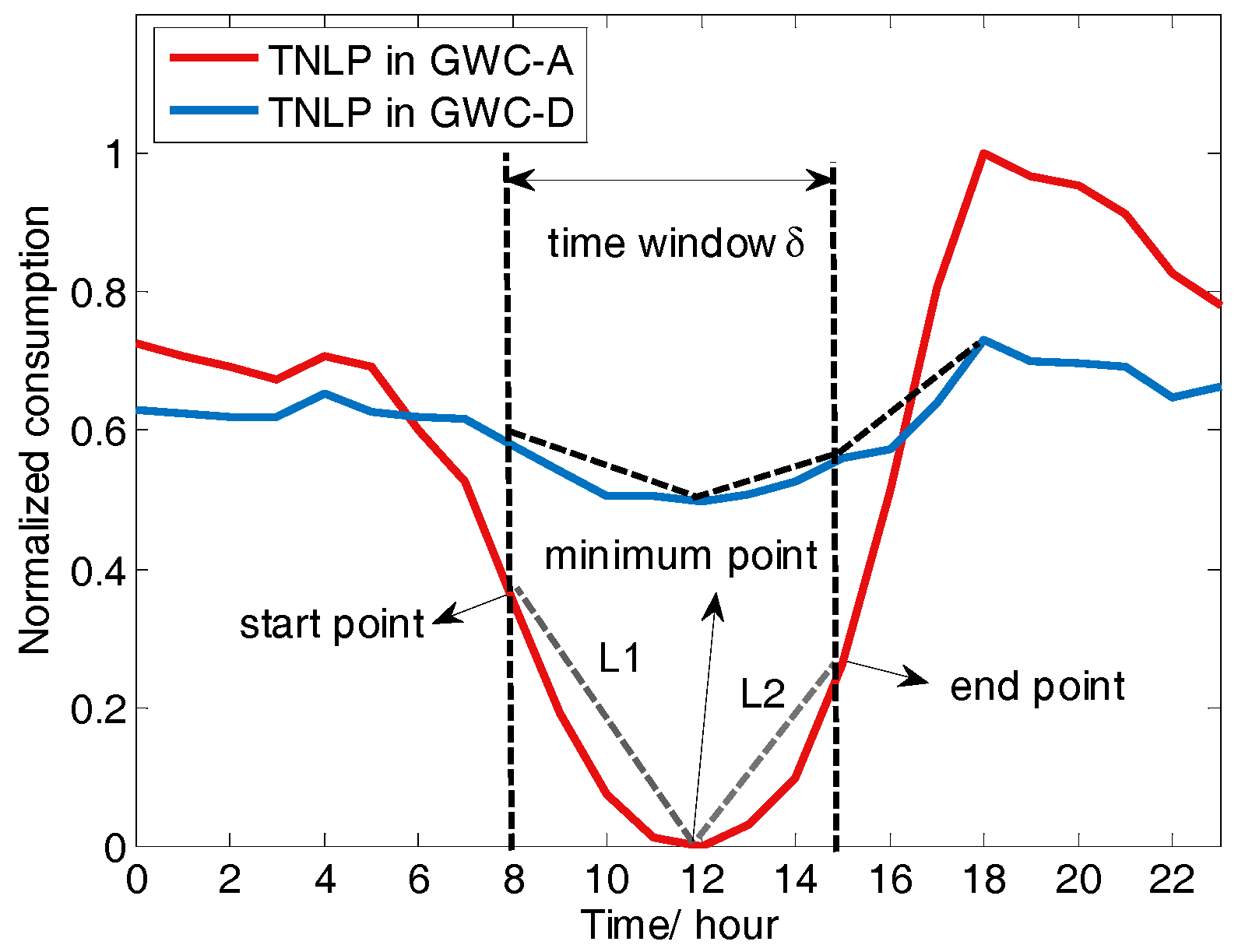
The second feature $F_2$ can only identify whether the $TNL{P}^A$ is concave or not. This feature will be ineffective in some cases, for example, some households without DPVSs but consume lower electricity in the midday. Hence, to further confirm whether the customer has a DPVS or not, other features should be extracted. The PV output power in different GWCs is different, thus the concavity degree of TNLP is also different in different GWCs. A new feature named concavity degree denoted by $F_3$ is extracted based on the above analysis. The specific process is illustrated as follows.

As shown in Figure 5, find a minimum point of the TNLP segment, denoted by $(t_m,TNLP(t_m))$. There are two lines $L_1$ and $L_2$ connecting this minimum point to the start point and the end point. Calculate the slope of these two lines, respectively. The sum of these two slopes can be used to describe the concavity degree:

$$\{\begin{array}{l}{k}_{\mathrm{A}}=|\frac{TNL{P}^A(t_s)-TNL{P}^A(t_m)}{t_s-t_m}|+\left|\frac{TNL{P}^A(t_e)-TNL{P}^A(t_m)}{t_e-t_m}\right|\\ k_{\mathrm{D}}=|\frac{TNL{P}^D(t_s)-TNL{P}^D(t_m)}{t_s-t_m}|+\left|\frac{TNL{P}^D(t_e)-TNL{P}^D(t_m)}{t_e-t_m}\right|\end{array}$$

(7)

$$F_3=k_{\mathrm{A}}/k_{\mathrm{D}}$$

(8)

For those customers with DPVSs, these two slopes should be different. That is, the value of $k_{\mathrm{A}}$ is much larger than $k_{\mathrm{D}}$. By contrast, the value of this feature will be close to 1 for customers without DPVSs, since there are no other load components are weather status driven.

3.3.4. Load Ramping Rate

The output power of DPVSs will rapidly decrease around the time of sunset, thus there will be a rapid increase in the net load curve. This phenomenon is defined as load ramping in this paper. To describe the ramping speed, an index named load ramping rate is defined, which is illustrated in Figure 6. Find a point $(t_f,TNLP(t_f))$ (it is set to be 19:00 in this paper) when the solar PV generation is close to 0, there is a line connecting this point and end point of time window $\mathbf{\delta }$, the slope of this line is defined as the load ramping rate. Apparently, the load ramping rate in different GWCs is different. Another feature denoted by $F_4$ is extracted according to the above analysis, expressed by Equations (9) and (10):

$$\{\begin{array}{l}R{T}_{\mathrm{A}}=\frac{TNL{P}^A(t_f)-TNL{P}^A(t_e)}{t_f-t_e}\\ R{T}_{\mathrm{D}}=\frac{TNL{P}^D(t_f)-TNL{P}^D(t_e)}{t_f-t_e}\end{array}$$

(9)

$$F_4=R{T}_{\mathrm{A}}/R{T}_{\mathrm{D}}$$

(10)

3.4. One-Class SVC Based DPVSD Model

A variety of supervised machine learning methods have been proposed to address classification and regression problems in the past years, such as SVM, artificial neural network (ANN) [19], K-Nearest Neighbor (KNN), Random Forests (RF), etc. Among these techniques, we choose SVM in this research due to its excellent performance in many applications (e.g., solar PV power forecasting [20,21]). SVM can be divided into two categories: SVC and SVR. The SVC model is used here because DPVSD is a classification problem.

The input of SVC model is the four features extracted in Section 3.3. The output is the label showing whether a customer has installed a DPVS or not. Specifically, the customers with DPVSs are marked as 1, while those customers without DPVSs are marked as 0. Radial basis function (RBF) is chosen as the kernel function in this paper.

4. Bootstrap-SVR Based DPVSCE Model

Once a DPVS is detected, the next step is to estimate its capacity. Similar to DPVSD, the DPVSCE also can be formulated as a supervised machine learning problem. The key to accurate estimation is still the feature extraction. Those features extracted for DPVSD focus on the difference between customers with DPVSs and those without are not effective for distinguishing DPVSs with different capacities. Therefore, new features should be extracted to describe the distinction between DPVSs with different capacities.

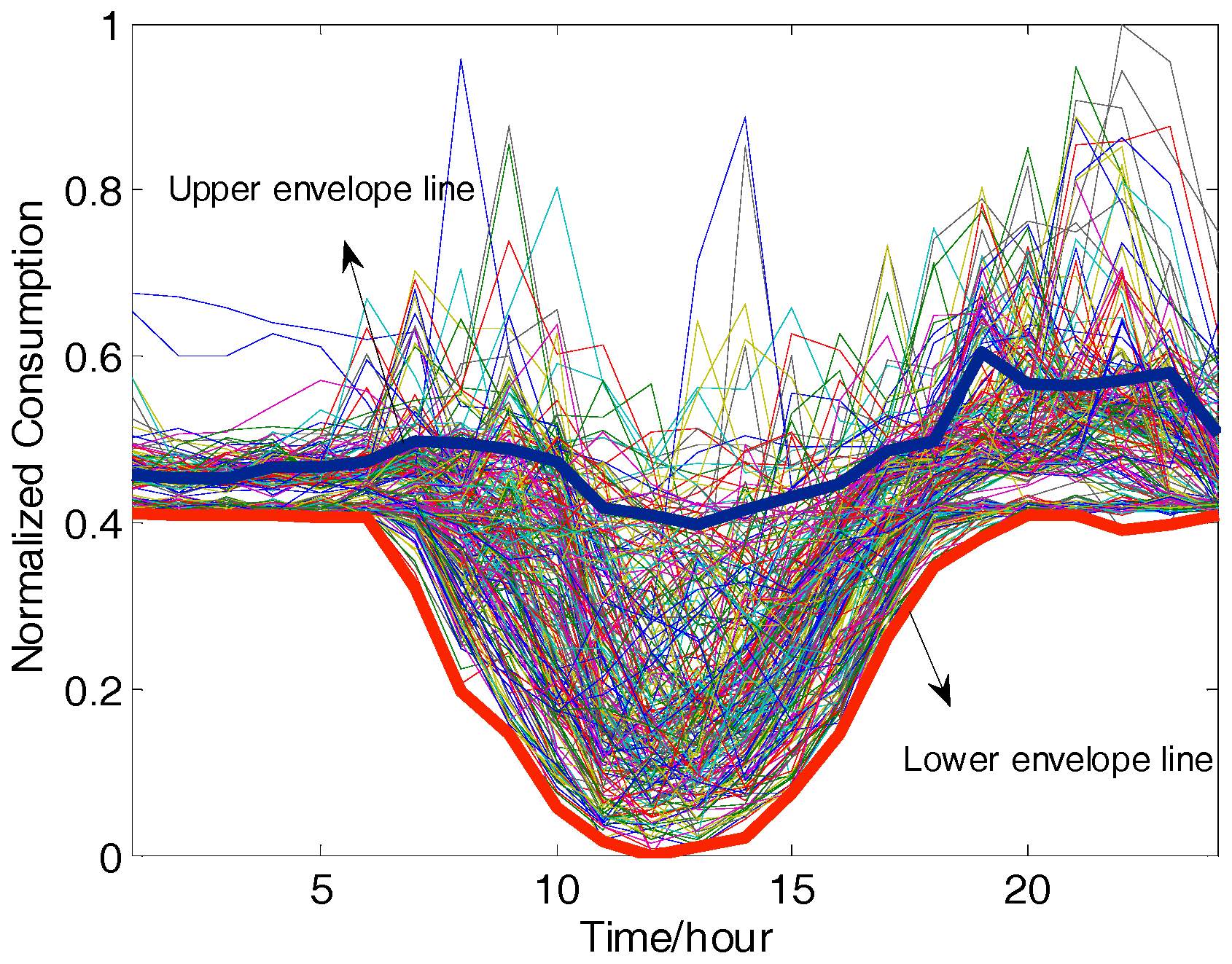
4.1. Extraction of Envelope Lines

One of the main differences between DPVSs with different capacities is the total amount of daily PV power generation. To estimate the daily total PV power generation only using the net load curves, two “special lines” need to be extracted from the net load curves for each customer. The first line defined as lower envelop line (LEL) should be able to reflect the net load level when the DPVS operates near to its maximum power generation capability. In contrast, the other line defined as upper envelope line (UEL) should be able to reflect the net load level when the DPVS output power is near to zero. These two envelope lines can be used to create features to describe the distinction between DPVSs with different capacities. The specific extraction process is illustrated as follows.

4.1.1. Extraction of LEL

Since GWC-A corresponds to the highest PV output power level among the four GWCs, all daily net load curves in GWC-A are used to extract the LEL. For each $t\in \mathit{T}$, find the minimum value $L_i^{-}(t)$ of all daily net load curves, expressed by Equation (11):

$$L^{-}(t)=\underset{d\in {\mathit{D}}_A}{\min }{P}_{net}(d,t),t\in \mathit{T}$$

(11)

As such, the LEL ${\mathit{L}}^{-}$ can be obtained by Equation (12):

$${\mathit{L}}^{-}=[L^{-}(1),L^{-}(2),\dots ,L^{-}(T)]$$

(12)

Apparently, this LEL reflects the net load level when the actual load level is minimum and the output power level of DPVS is maximum.

4.1.2. Extraction of UEL

A suitable UEL should be able to represent the net load level when the PV output power is minimum and the actual load level is minimum. Since GWC-D corresponds to the lowest PV output power level, all daily net load curves in GWC-D are used to extract the UEL. Similarly, for each $t\in \mathit{T}$, we calculate the minimum value of all net load curves to obtain the UEL ${\mathit{L}}^{+}$, given by Equations (13) and (14).

$$L^{+}(t)=\underset{d\in {\mathit{D}}_D}{\min }(P_{net}(d,t))$$

(13)

$${\mathit{L}}^{+}=[L^{+}(1),L^{+}(2),\dots ,L^{+}(T)]$$

(14)

An example of envelope lines extraction is shown in Figure 7.

4.2. Extremum Difference Based Feature Extraction

Three features reflecting the size of DPVS capacity can be extracted based on the obtained LEL and UEL. To obtain the most obvious features for estimation, the influence from the part of load curve within which DPVS is unable to produce electricity should be avoided. So we still use the segment within the time period $\mathbf{\delta }$ of the envelop line to extract features.

4.2.1. Minimum Net Load Power

The first feature denoted by $F_1^{DPVE}$ is equal to the minimum value of the LEL, which is given by Equation (15):

$$F_1^{DPVE}=\min (L^{-}(t)),t\in \mathbf{\delta }$$

(15)

This feature can be used to describe the maximum DPVS generation capacity. Apparently, when the electricity consumption levels of two customers are same, smaller $F_1^{DPVE}$ indicates a larger DPVS capacity.

4.2.2. Maximum Difference of PV Output Power

The second feature denoted by $F_2^{DPVE}$ is defined as the maximum value of the difference between UEL and LEL, given by Equation (16):

$$F_2^{DPVE}=\max (L^{+}(t)-L^{-}(t)),t\in \mathbf{\delta }$$

(16)

4.2.3. Total PV Power Generation during Time Window

The area between UEL and LEL can be used to characterize the solar PV generation and distinguish different DPVSs with different capacities. Hence, this index is selected as the third feature denoted by $F_3^{DPVE}$, which can be calculated by Equation (17):

$$F_3^{DPVE}={\displaystyle {\int }_{t=t_s}^{t=t_e}(L^{+}(t)-L^{-}(t))dt}$$

(17)

4.3. Bootstrap-SVR Based DPVSCE Model

Since the DPVS capacity is numerically continuous, hence regression model can be used to estimate it. To achieve higher estimation accuracy, sufficient data is usually needed for training. However, it is common in practice that the dataset is imbalanced, i.e., not uniformly distributed. The imbalanced dataset will not only significantly affect the accuracy of classification model, but also has a negative impact on the performance of the regression model. To address this issue, a bootstrap-SVR based DPVSCE model is proposed in this paper.

First, the typical output power (TOP) curve of a local DPVS with capacity of 1 kWp is defined as $P_{TPV}(d,t),d\in \mathit{D},t\in \mathit{T}$. It can be approximated by those authorized customers whose DPVS capacity and the output power are known. The output power of DPVSs with various capacities can be simulated by TOP, as follows:

$$P_{pv}^s(d,t)=C^s{P}_{TPV}(d,t),d\in \mathit{D},t\in \mathit{T}$$

(18)

where $C^s$ is the simulated capacity and $P_{pv}^s(d,t)$ is the simulated output power of the DPVS with capacity of $C^s$.

Second, bootstrap method is used to simulate more electricity consumption data from the known samples. The core of bootstrap is resampling with replacement, which is particularly useful when there is a small amount of empirical data. In this way, various samples can be obtained.

Finally, a large number of net load profiles covering all distribution of DPVS capacities can be obtained through the random combination of the various simulated output power and the electricity consumption data.

Similar to the SVC-based DPVSD model, the input of the SVR is the three extracted features. The output is the corresponding actual DPVS capacity.

5. Case Study

5.1. Dataset

The dataset used in this research is obtained from the Pecanstreet Database which collects consumer energy recorded from residential houses in Austin (Texas, U.S.A.) [22]. In this paper, the smart meter readings containing electricity consumption data, PV output power data, and net load data with the sampling interval of 1 h from 183 households with rooftop solar systems in 2015 are used to test and verify the proposed approach.

5.2. Performance Metric

To evaluate the proposed DPVSD and DPVSCE models, several performance metrics are adopted.

5.2.1. Performance Metric for DPVSD Model

Confusion matrix is usually used to evaluate a classification model, which contains all the information about actual and predicted classes:

$$M=\left[\begin{array}{l}{m}_{11}\dots \dots m_{1N}\\ .......\\ m_{N1}\dots \dots m_{NN}\end{array}\right]=[m_{ij}]i,j=1,\dots \dots ,N$$

(19)

where $m_{ij}$ is the number of objects which actually belong to the class $i$ but be classified to the class $j$, $N$ is the number of total classes.

Performance of classification model is commonly evaluated by the following three indexes: product’s accuracy (PA), user’s accuracy (UA) and overall accuracy (OA) using the data in confusion matrix:

$$P{A}_i=\frac{m_{ii}}{{\displaystyle {\sum }_{j=1}^N{m}_{ij}}},i=1,\dots \dots ,N$$

(20)

$$U{A}_i=\frac{m_{ii}}{{\displaystyle {\sum }_{j=1}^N{m}_{ji}}},i=1,\dots \dots ,N$$

(21)

$$OA=\frac{{\displaystyle {\sum }_{i=1}^N{m}_{ii}}}{{\displaystyle {\sum }_{i=1}^N{\displaystyle {\sum }_{j=1}^N{m}_{ij}}}}$$

(22)

PA is used to describe the classification accuracy of one specific actual class. UA is the indicator to describe the correct identified ratio of one specific output class. OA is used to describe the classification accuracy of all actual classes or the correct identified ratio of all output classes.

5.2.2. Performance Metric for DPVSCE Model

Two indicators defined in Equations (23) and (24) are adopted to evaluate the performance of the proposed DPVSCE model:

$$MAPE=\frac{1}{N}{\displaystyle \sum _{n=1}^N\left|\frac{C_n^p-C_n^a}{C_n^a}\right|}$$

(23)

$$R^2=\frac{{\left(N{\displaystyle \sum _{n=1}^N\left(C_n^p{C}_n^a\right)}-{\displaystyle \sum _{n=1}^N{C}_n^p}{\displaystyle \sum _{n=1}^N{C}_n^a}\right)}^2}{\left(N{\displaystyle \sum _{n=1}^N{\left(C_n^p\right)}^2}-{\left({\displaystyle \sum _{n=1}^N{C}_n^p}\right)}^2\right)\left(N{\displaystyle \sum _{n=1}^N{\left(C_n^a\right)}^2}-{\left({\displaystyle \sum _{n=1}^N{C}_n^a}\right)}^2\right)}$$

(24)

where $C_n^a$ and $C_n^p$ represent the actual and predict capacity of the nth test sample, respectively. Smaller MAPE values indicate better performance of the DPVSCE model. The larger the $R^2$ is, the better the model is.

5.3. Experiment Design

In this section, two experiments are designed to test and verify the effectiveness of the proposed approach. Experiment 1 is designed for testing the performance of the proposed DPVSD model and the other one is for the DPVSCE model.

5.3.1. Experiment 1: Performance Test of the DPVSD Model

To test the performance of the proposed DPVSD model, some electricity consumption data of those customers without DPVSs is needed. Since the dataset used contains the total electricity use data of each customer. Hence, it is feasible to simulate some virtual customers without DPVSs by using the total electricity use data. As such, another 183 customers without DPVSs can be obtained. In order to make the results reliable, we use the K cross-validation technique. These 366 customers are randomly divided into 4-folds (about 92 samples for each fold). The SVM classifier is then trained (using three folds) and evaluated (using one fold) four times. The four results from the 4-folds are averaged to produce a single result. The above procedure is run 100 rounds and the performance metrics are calculated and recorded for each round. The simulation of the SVC-based DPVSD model is implemented using MATLAB R2014a (MathWorks, Natick, MA, USA) and LIBSVM tools (Version 3.17). The grid search method is adopted to optimize the penalty parameter c and kernel parameter of RBF.

In order to illustrate the advantage of the proposed voting method for GWC label generation, a comparison is conducted between the voting method and the simple clustering method (i.e., just use the output power data from a single DPVS to generate the GWC label). The comparison results of these two methods in different cases are shown in

Table 1. The classification evaluation results of the proposed DPVSD model in different cases: a comparison between two GWC label generation methods.

GWC Label Generation Based on the Output Power Data from Single PV System
Label	Performance Metrics	Best (%)	Average (%)	Worst (%)
Label = 1	PA1	95.35	91.33	84.44
	UA1	100	97.25	95.74
Label = 0	PA2	100	97.05	95.00
	UA2	96.08	90.76	86.54
OA		97.83	93.73	90.22
GWC Label Generation Based on the Voting Method
Label = 1	PA1	100	92.04	84.44
	UA1	100	98.89	95.74
Label = 0	PA2	100	98.96	95.00
	UA2	100	92.61	86.54
OA		100	95.51	90.22

. Several findings can be summarized as follows. First, the proposed voting method achieves more accurate classification results than the simple clustering method in terms of the best and average cases. This finding verifies our hypothesis that the labels generated by multi-sources are more reliable. Second, the DPVSD model presents very good overall performance in all cases. The OA of the proposed method can reach 100% in the best case. Even in the worst case, the proposed DPVSD also can achieve a high accuracy of 90.22%, which verifies the effectiveness of the proposed features.

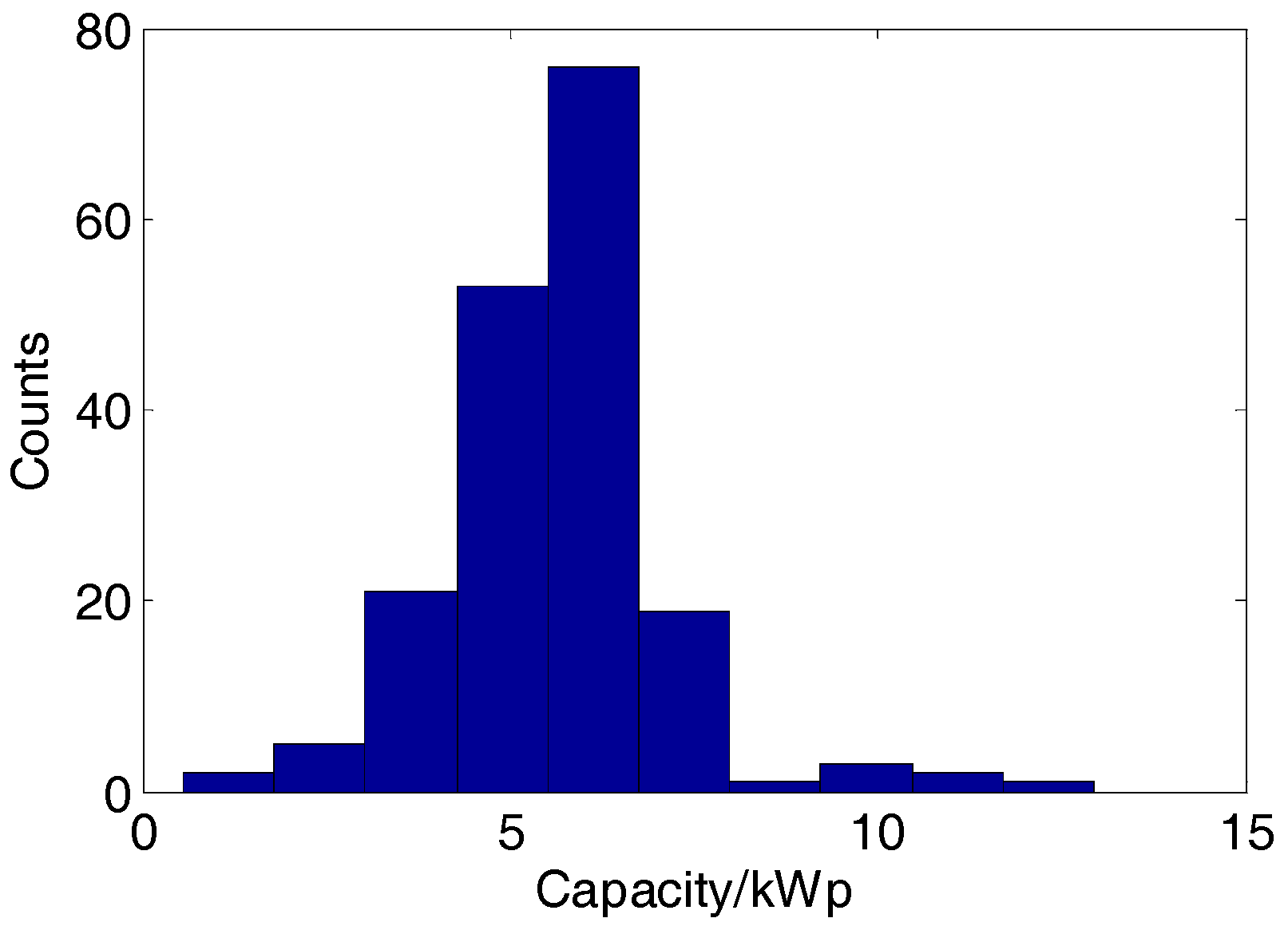
5.3.2. Experiment 2: Performance Test of the DPVSCE Model

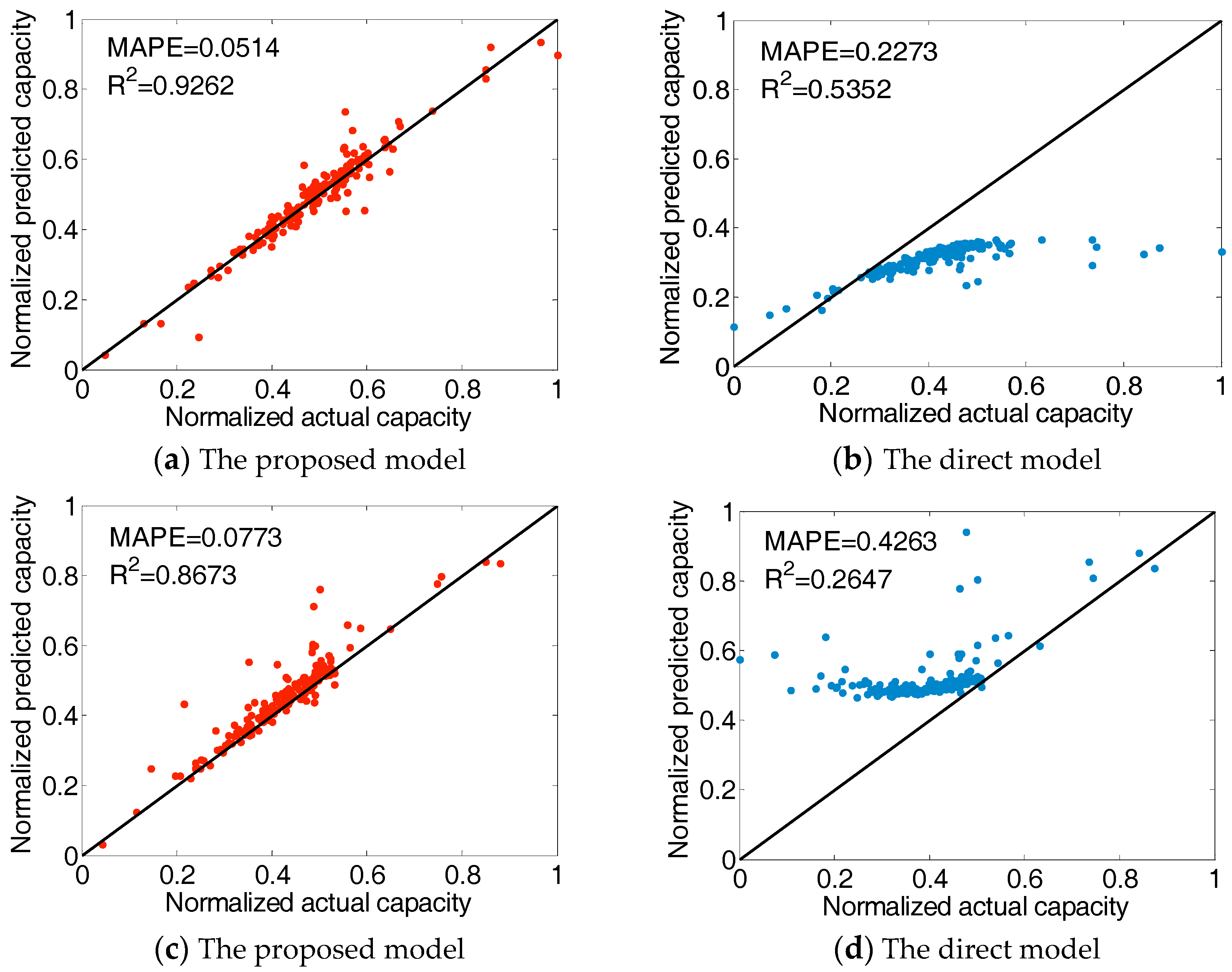
The distribution of DPVS capacities for the 183 customers is shown in Figure 8. These customers can be divided into three groups according to their DPVSs capacities: “small” (<4 kWp), “middle” (4–6 kWp) and “large” (>6 kWp). Apparently, the customers in the “middle” group account for the largest proportion (about 70%). To test the performance of the proposed DPVSCE model in such an imbalance dataset, 10 customers are randomly selected from the “small” group and “large” group for training, the other 173 customers are used for testing. 1000 virtual customers are generated by the bootstrap method. The proposed bootstrap-SVR model is compared with the direct SVR model i.e., directly using the training samples to train the model. The comparison results are shown in Figure 9. It can be seen that the proposed bootstrap-SVR model presents high accuracy estimation results in both cases. The value of MAPE is only between 5~7% and the value of $R^2$ is between 0.86~0.92. However, in terms of the direct model, it shows biased estimation results in both cases. Specifically, large errors occur when only the samples in “small” or “large” group are used for training, which reveals the low adaptability of direct model to imbalance dataset.

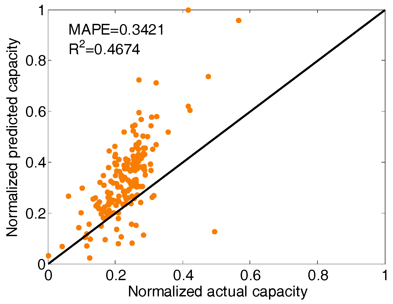
Furthermore, we also compare our DPVSCE method with the method proposed in the literature [16] on this dataset. The estimation results of the method proposed in that literature is shown in Figure 10. It produced large estimation errors and the value of MAPE is up to 34%. It is pointed in that literature that it is almost impossible to get an accurate DPVS capacity estimation without the local cloud cover index information. For our method, high estimation accuracy can be achieved without any weather information and very few training samples are required in our method.

6. Discussion

In this section, we analyze the relative importance of the proposed features for both classification and capacity estimation and further test the robustness of the proposed method under several scenarios.

6.1. Correlation Analysis

The input feature showing more strong correlation with the output is usually considered as a more important feature [23]. Maximal information coefficient (MIC) is used to analyze the relative importance of the proposed input features for both classification and capacity estimation, which can not only quantify the linear relation but also quantify the non-linear relation between two variables [24]. The analysis results are shown in

Table 2. The MIC values between the four features used for classification and classification label.

Feature	$F_1$	$F_2$	$F_3$	$F_4$
MIC value	0.688	0.445	0.565	0.367

and

Table 3. The MIC values between the three features used for estimation and capacity values.

Feature	$F_1^{DPVE}$	$F_2^{DPVE}$	$F_3^{DPVE}$
MIC value	0.937	0.505	0.602

, respectively.

From Table 2, we can see that correlation between classification label and (i.e., Ratio of total electricity consumption in GWC-A to GWC-D) is stronger than others, which indicates it is the most important feature for classification model. (i.e., load ramping rate) shows the weakest correlation, which indicates it is relatively unimportant compared with other features.

It is shown in Table 3 that the order of relative importance of the proposed three feature for capacity estimation is $F_1^{DPVE}>F_3^{DPVE}>F_2^{DPVE}$.

6.2. The Impact of Energy Storage on DPVSD Model

Some loads such as energy storage devices (ESDs) can act as generators in some cases, which will also reshape the load profiles and probably affect the detection results of the DPVSD model. To test the robustness of the proposed DPVSD model, a scenario in which some customers have ESDs but without DPVSs is designed.

The Powerwall, a household ESD produced by Tesla is selected for simulation [25]. The useable storage capacity of the Powerwall is 10 kWh. In our simulation, the EBS is set to charge in the low electricity price period (0:00–6:00) and discharge in the high electricity price period (12:00–20:00) for each day. The charging/discharging power is set to be 5 kW and the duration of charging/discharging is set to be 2 h. Assume that all customers without DPVS have installed an ESD. The simulated normalized TNLPs of a customer after introducing a household ESD are shown in Figure 11. The classification accuracy of the proposed DPVSD model after introducing ESDs is shown in

Table 4. The classification accuracy after introducing ESDs.

Label	Performance Metrics	Best (%)	Average (%)	Worst (%)
Label = 1	PA1	93.18	83.92	80.00
	UA1	95.35	96.20	97.78
Label = 0	PA2	95.83	97.05	97.30
	UA2	93.88	85.48	76.60
OA		94.57	90.16	86.96

.

It can be overserved from Table 4 that the proposed DPVSD model can still achieve high detection accuracy after introducing the ESDs. This is because that the charging/discharging behaviors are not weather status driven. Hence, as shown in Figure 11, the TNLPs of a customer without DPVS in different GWC are similar. The extracted features can accurately reflect the unique WSDDFs of DPVSs so that the DPVSs can be distinguished with the ESDs.

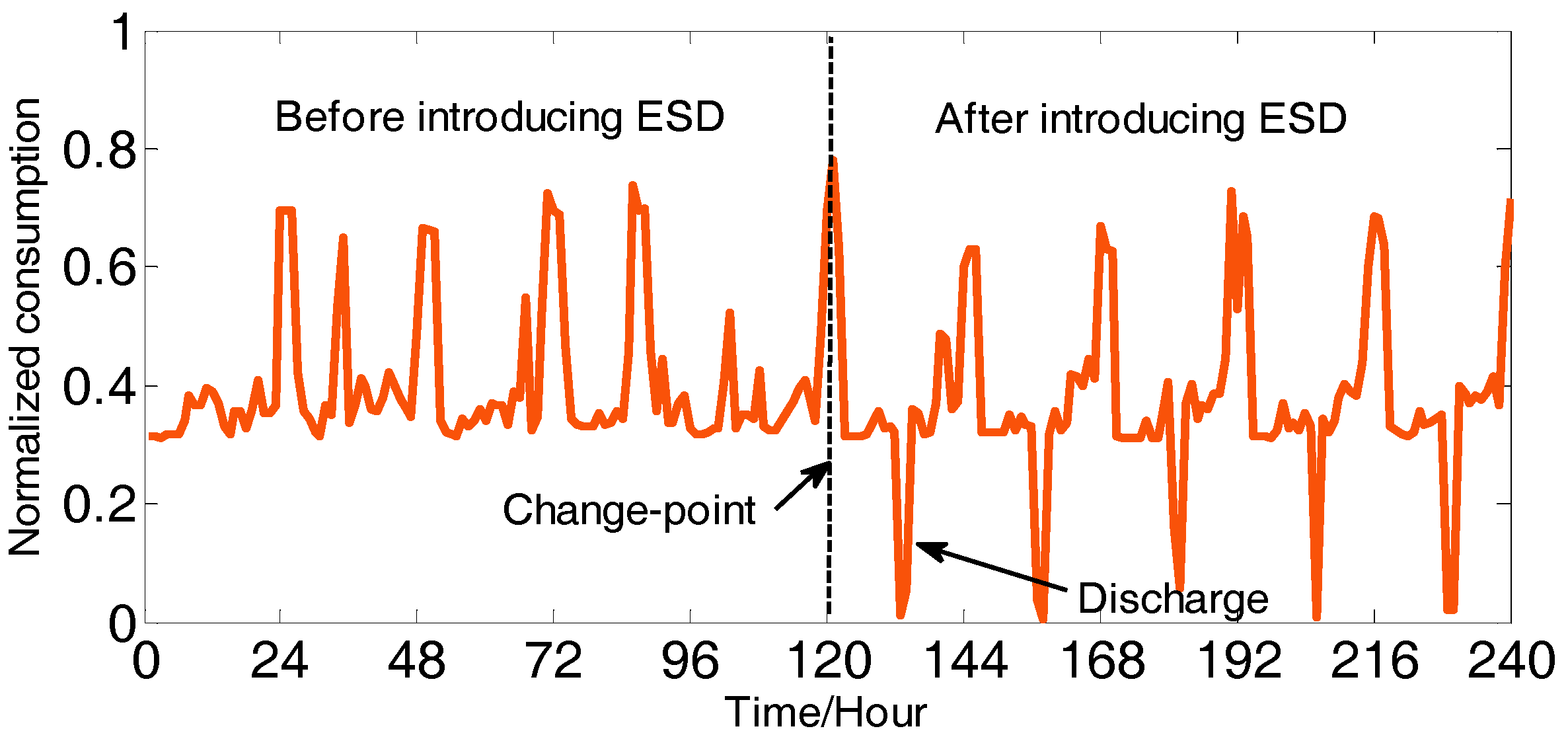
Figure 12 presents the simulated net load profiles for 10 consecutive days. Assume the ESD is introduced in the 6th day, there is a high possibility for the change-point detection algorithm to identify this customer as a DPVS owner in this case. The daily net load profiles after introducing the ESDs are totally different with before. Hence, a change-point will be detected by the algorithm. Moreover, the concave-down net load profiles caused by the discharging of ESD make them difficult to be distinguished from those DPVS owners.

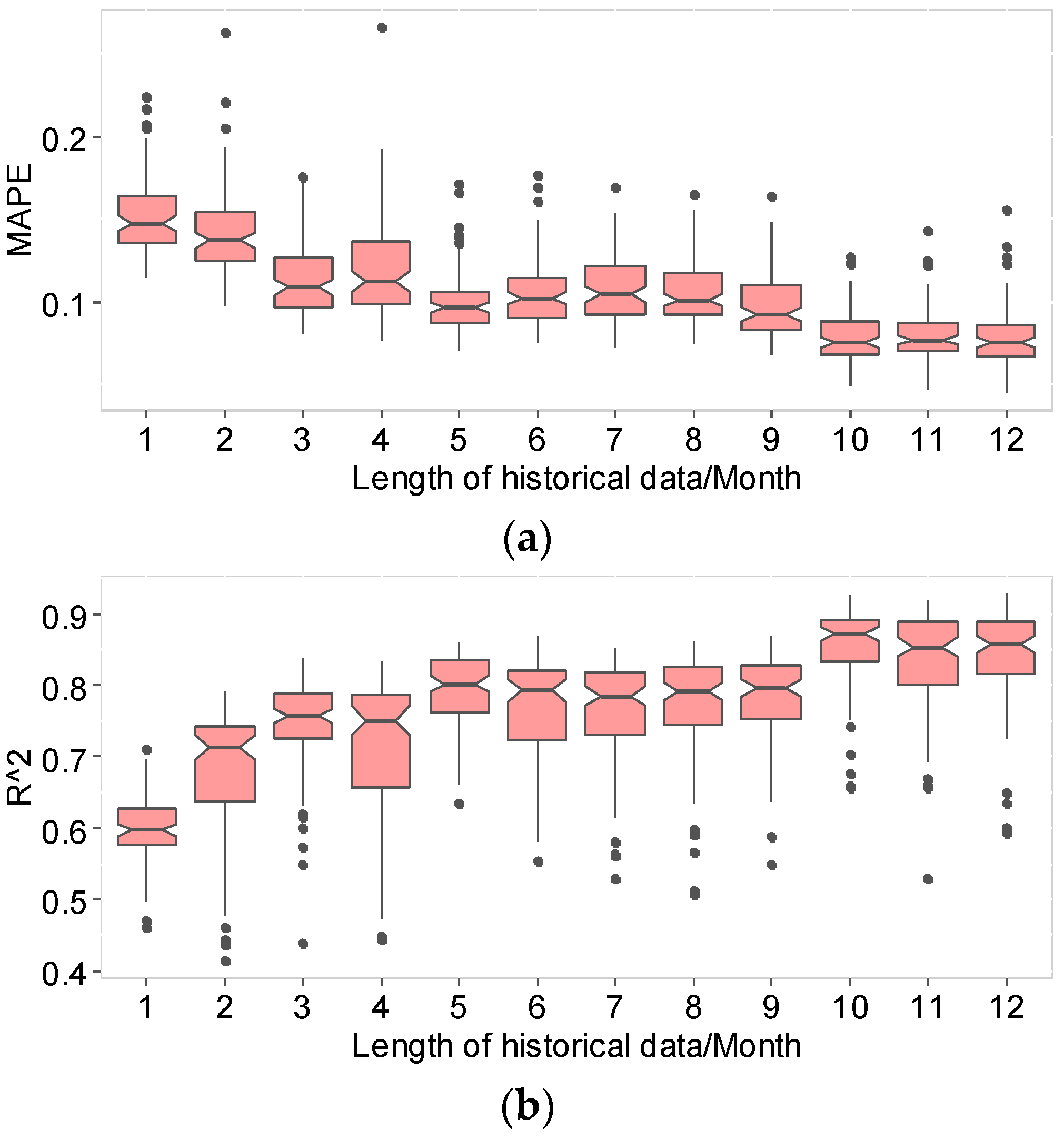
6.3. The Impact of Length of Historical Data on the DPVSCE Model

Various lengths of historical data from 1 month up to 12 months are set to explore its impact on the performance of the proposed DPVSCE method. The model is run 100 rounds for each length and MAPE and $R^2$ are calculated in each round. The distribution for the estimation results of 100 rounds is presented in Figure 13.

We find that both of MAPE and $R^2$ become worse with the decrease of the available historical data. The value of MAPE and $R^2$ are 15% and 0.6, respectively, in the worst case, i.e., only one month of data can be used. The above findings indicate that the proposed approach relies on the historical data. Hence, it’s better to obtain sufficient data to achieve higher accuracy in practice. However, the proposed approach still outperforms the model proposed in the literature [16] even with limited historical data.

7. Conclusions

In this paper, a two-stage DPVS capacity estimation approach was proposed. In the first stage, a one-class SVC-based DPVSD model was proposed to detect whether a customer has a DPVS or not. In the second stage, a bootstrap-SVR model without the requirement of a large number of training data and any weather information is proposed to further estimate the capacities of the detected DPVSs. A realistic dataset from Austin (TX, U.S.A.) consisting of 183 residential customers with DPVSs was used to test the performance of the proposed approach. The results showed that the proposed approach had very good overall performance. Moreover, the proposed DPVSCE model can well accommodate to the imbalance dataset. Furthermore, we also investigated the impact of household ESDs and lengths of available historical data on the performance of the proposed approach. The result indicated that the proposed DPVSD model was robust to the existence of ESDs. The proposed DPVSCE model relied on the length of historical data. To achieve higher accuracy of the DPVS estimation results, sufficient historical data is usually needed. However, our method still outperforms the current estimation methods even with limited historical data.

Future work possibilities are as follows:

• Testing the proposed approach in other sites with different latitudes and user profiles to further verify its effectiveness.
• Explore DPVS output power simulation methods to improve the performance of the DPVSCE model in the case of limited historical data.
• Investigating the robustness of the proposed approach in the presence of DR (e.g., the TOU price DR [26]).
• Extending the proposed approach to detect the orientation of the installed PV to check whether the PV system is operating on the optimal orientation.

References

- Preliminary Market Report. Available online: http://www.iea-pvps.org/index.php?id=266 (accessed on 21 April 2018).
- National Survey Reports, International Energy Agency Photovoltaic Power Systems Programme. Available online: http://www.iea-pvps.org/index.php?id=93 (accessed on 21 April 2018).
- Wang, F.; Xu, H.; Xu, T.; Li, K.; Shafie-khah, M.; João, P.S.; Catalão, J.P.S. The values of market-based demand response on improving power system reliability under extreme circumstances. Appl. Energy 2017, 193, 220–231. [Google Scholar] [CrossRef]
- Chen, Q.; Wang, F.; Hodge, B.M.; Zhang, J.; Li, Z.; Shafie-Khah, M.; Catalao, J.P.S. Dynamic Price Vector Formation Model-Based Automatic Demand Response Strategy for PV-Assisted EV Charging Stations. IEEE Trans. Smart Grid 2017, 8, 2903–2915. [Google Scholar] [CrossRef]
- Wang, F.; Liu, L.; Yu, Y.; Li, G.; Li, J.; Shafie-khah, M.; Catalão, J. Impact Analysis of Customized Feedback Interventions on Residential Electricity Load Consumption Behavior for Demand Response. Energies 2018, 11, 770. [Google Scholar] [CrossRef]
- Talari, S.; Shafie-khah, M.; Wang, F.; Aghaei, J.; Catalao, J.P.S. Optimal Scheduling of Demand Response in Pre-emptive Markets based on Stochastic Bilevel Programming Method. IEEE Trans. Ind. Electron. 2017. [Google Scholar] [CrossRef]
- Wang, F.; Li, K.; Liu, C.; Mi, Z.; Shafie-khah, M.; Catalao, J.P.S. Synchronous Pattern Matching Principle Based Residential Demand Response Baseline Estimation: Mechanism Analysis and Approach Description. IEEE Trans. Smart Grid 2018. [Google Scholar] [CrossRef]
- Wijaya, T.K.; Vasirani, M.; Aberer, K. When bias matters: An economic assessment of demand response baselines for residential customers. IEEE Trans. Smart Grid 2014, 5, 1755–1763. [Google Scholar] [CrossRef]
- Kaur, A.; Pedro, H.T.C.; Coimbra, C.F.M. Impact of onsite solar generation on system load demand forecast. Energy Convers. Manag. 2013, 75, 701–709. [Google Scholar] [CrossRef]
- Massidda, L.; Marrocu, M. Decoupling Weather Influence from User Habits for an Optimal Electric Load Forecast System. Energies 2017, 10, 2721. [Google Scholar] [CrossRef]
- Yu, Y.; Wen, X.; Zhao, J.; Xu, Z.; Li, J. Co-Planning of Demand Response and Distributed Generators in an Active Distribution Network. Energies 2018, 11, 354. [Google Scholar] [CrossRef]
- Yang, Y.; Wang, X.; Luo, J.; Duan, J.; Gao, H.; Xiao, X. Multi-Objective Coordinated Planning of Distributed Generation and AC/DC Hybrid Distribution Networks Based on a Multi-Scenario Technique Considering Timing Characteristics. Energies 2017, 10, 2137. [Google Scholar] [CrossRef]
- EIA Electricity Data Now Include Estimated Small-Scale Solar PV Capacity and Generation. Available online: https://www.eia.gov/todayinenergy/detail.cfm?id=23972 (accessed on 1 December 2018).
- Hawaiian Electric. Hawaiian Electric Asking Customers with Unauthorized Rooftop PV Systems to Disconnect to Ensure Safety, Fairness for All. Available online: https://www.hawaiianelectric.com/hawaiian-electric-asking-customers-with-unauthorized-rooftop-pv-systems-to-disconnect-to-ensure-safety-fairness-for-all (accessed on 3 June 2018).
- Malof, J.M.; Bradbury, K.; Collins, L.M.; Newell, R.G. Automatic detection of solar photovoltaic arrays in high resolution aerial imagery. Appl. Energy 2016, 183, 229–240. [Google Scholar] [CrossRef] [Green Version]
- Zhang, X.; Grijalva, S. A Data-Driven Approach for Detection and Estimation of Residential PV Installations. IEEE Trans. Smart Grid 2016, 7, 2477–2485. [Google Scholar] [CrossRef]
- Wang, F.; Zhen, Z.; Mi, Z.; Sun, H.; Su, S.; Yang, G. Solar irradiance feature extraction and support vector machines based weather status pattern recognition model for short-term photovoltaic power forecasting. Energy Build. 2015, 86, 427–438. [Google Scholar] [CrossRef]
- Sun, Y.; Wang, F.; Wang, B.; Chen, Q.; Engerer, N.; Mi, Z. Correlation Feature Selection and Mutual Information Theory Based Quantitative Research on Meteorological Impact Factors of Module Temperature for Solar Photovoltaic Systems. Energies 2017, 10, 7. [Google Scholar] [CrossRef]
- Wang, F.; Mi, Z.; Su, S.; Zhao, H. Short-term solar irradiance forecasting model based on artificial neural network using statistical feature parameters. Energies 2012, 5, 1355–1370. [Google Scholar] [CrossRef]
- Wang, F.; Zhen, Z.; Wang, B.; Mi, Z. Comparative Study on KNN and SVM Based Weather Classification Models for Day Ahead Short Term Solar PV Power Forecasting. Appl. Sci. 2017, 8, 28. [Google Scholar] [CrossRef]
- Wang, F.; Zhen, Z.; Liu, C.; Mi, Z.; Hodge, B.M.; Shafie-khah, M.; Catalão, J.P.S. Image phase shift invariance based cloud motion displacement vector calculation method for ultra-short-term solar PV power forecasting. Energy Convers. Manag. 2018, 157, 123–135. [Google Scholar] [CrossRef]
- PECAN STREET. Available online: http://www.pecanstreet.org/what-is-pecan-street-inc/ (accessed on 15 September 2017).
- Wang, F.; Li, K.; Duić, N.; Mi, Z.; Hodge, B.M.; Shafie-khah, M.; Catalão, J.P.S. Association rule mining based quantitative analysis approach of household characteristics impacts on residential electricity consumption patterns. Energy Convers. Manag. 2018, 171, 839–854. [Google Scholar] [CrossRef]
- Reshef, D.N.; Reshef, Y.A.; Finucane, H.K.; Grossman, S.R.; McVean, G.; Turnbaugh, P.J.; Lander, E.S.; Mitzenmacher, M.; Sabeti, P.C. Detecting novel associations in large data sets. Science 2011, 334, 1518–1524. [Google Scholar] [CrossRef] [PubMed]
- Powerwall. Available online: https://www.tesla.com/powerwall (accessed on 12 September 2017).
- Wang, F.; Zhou, L.; Ren, H.; Liu, X.; Shafie-khah, M. Multi-objective Optimization Model of Source-Load-Storage Synergetic Dispatch for Building Energy System Based on TOU Price Demand Response. IEEE Trans. Ind. Appl. 2018, 54, 1017–1028. [Google Scholar] [CrossRef]
© 2018 by the authors. Licensee MDPI, Basel, Switzerland. This article is an open access article distributed under the terms and conditions of the Creative Commons Attribution (CC BY) license (http://creativecommons.org/licenses/by/4.0/).