Full- and Reduced-Order State-Space Modeling of Wind Turbine Systems with Permanent Magnet Synchronous Generator

 ,
,  , and
, and
Abstract
1. Introduction
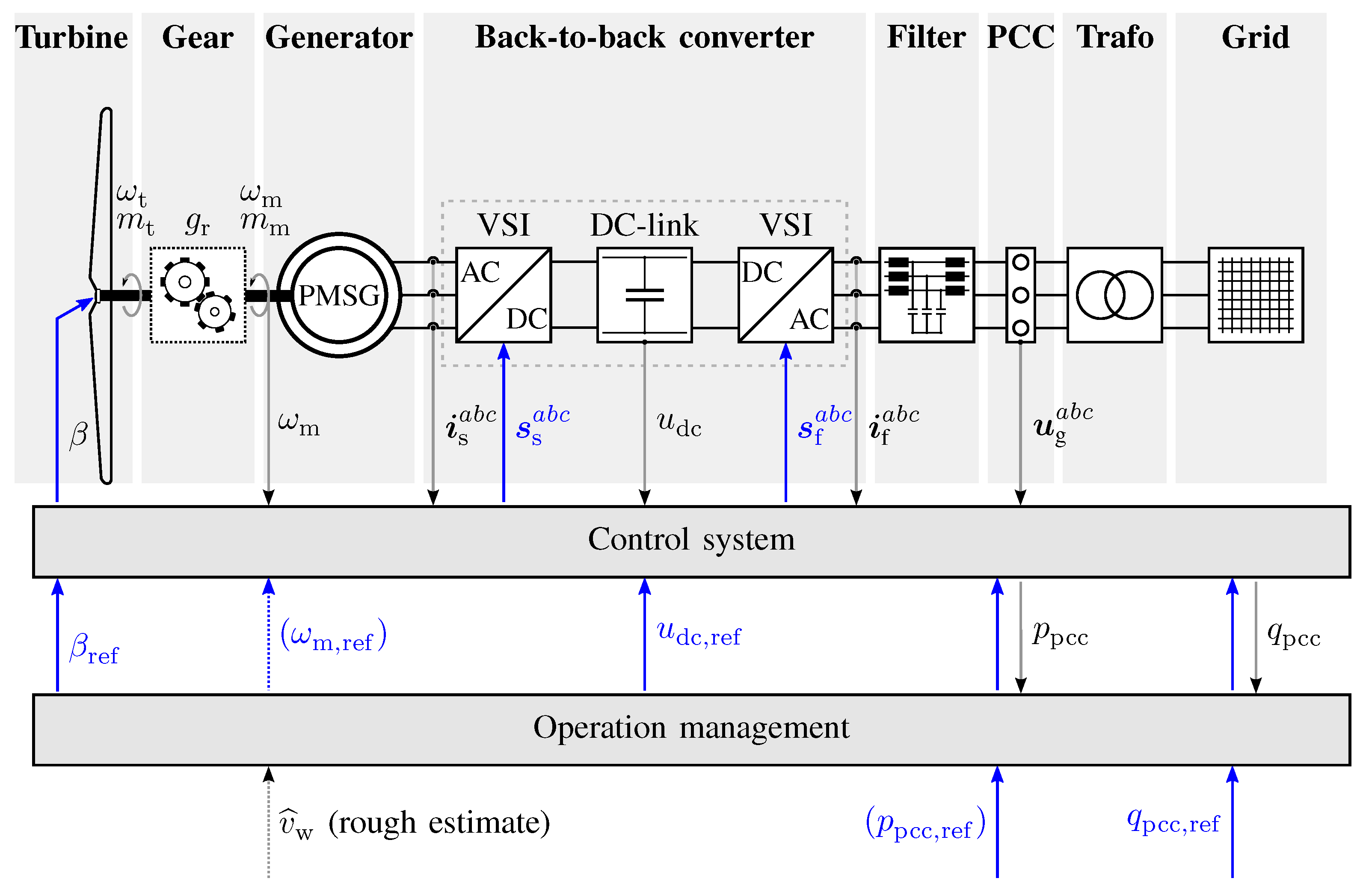
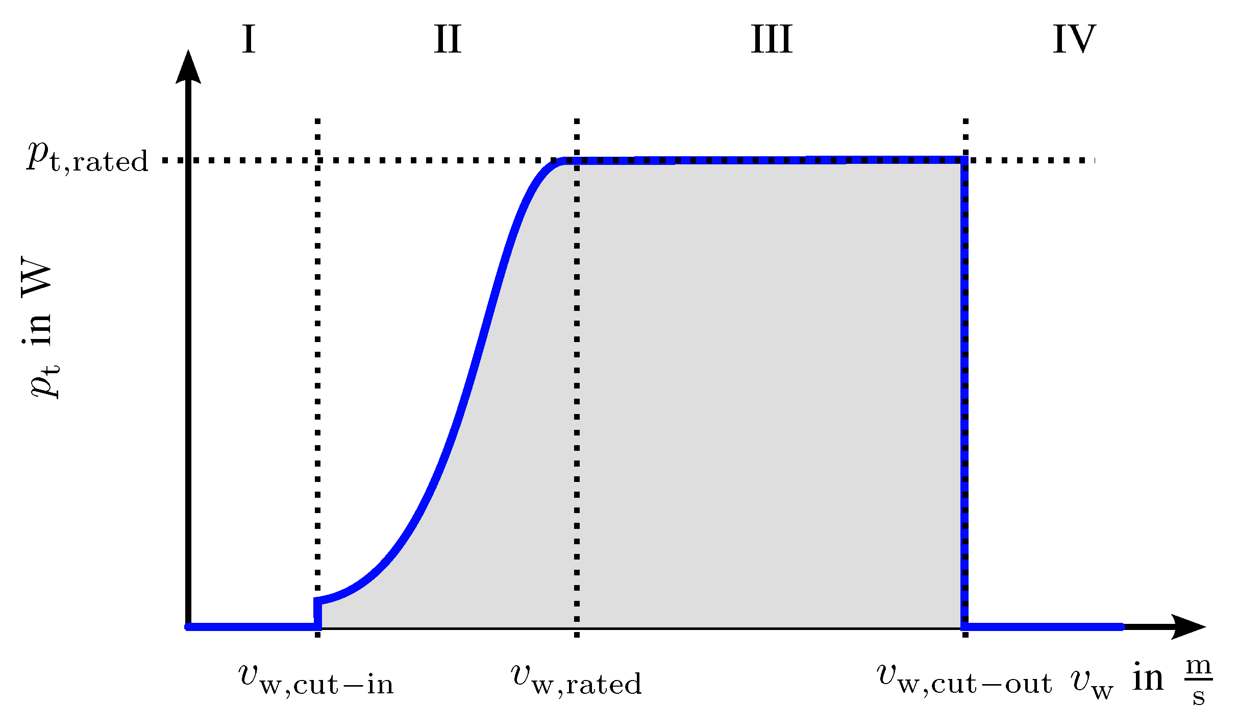
2. System Description
3. Full-Order Models
3.1. Aerodynamics, Turbine Torque and Drive Train
3.1.1. Aerodynamics
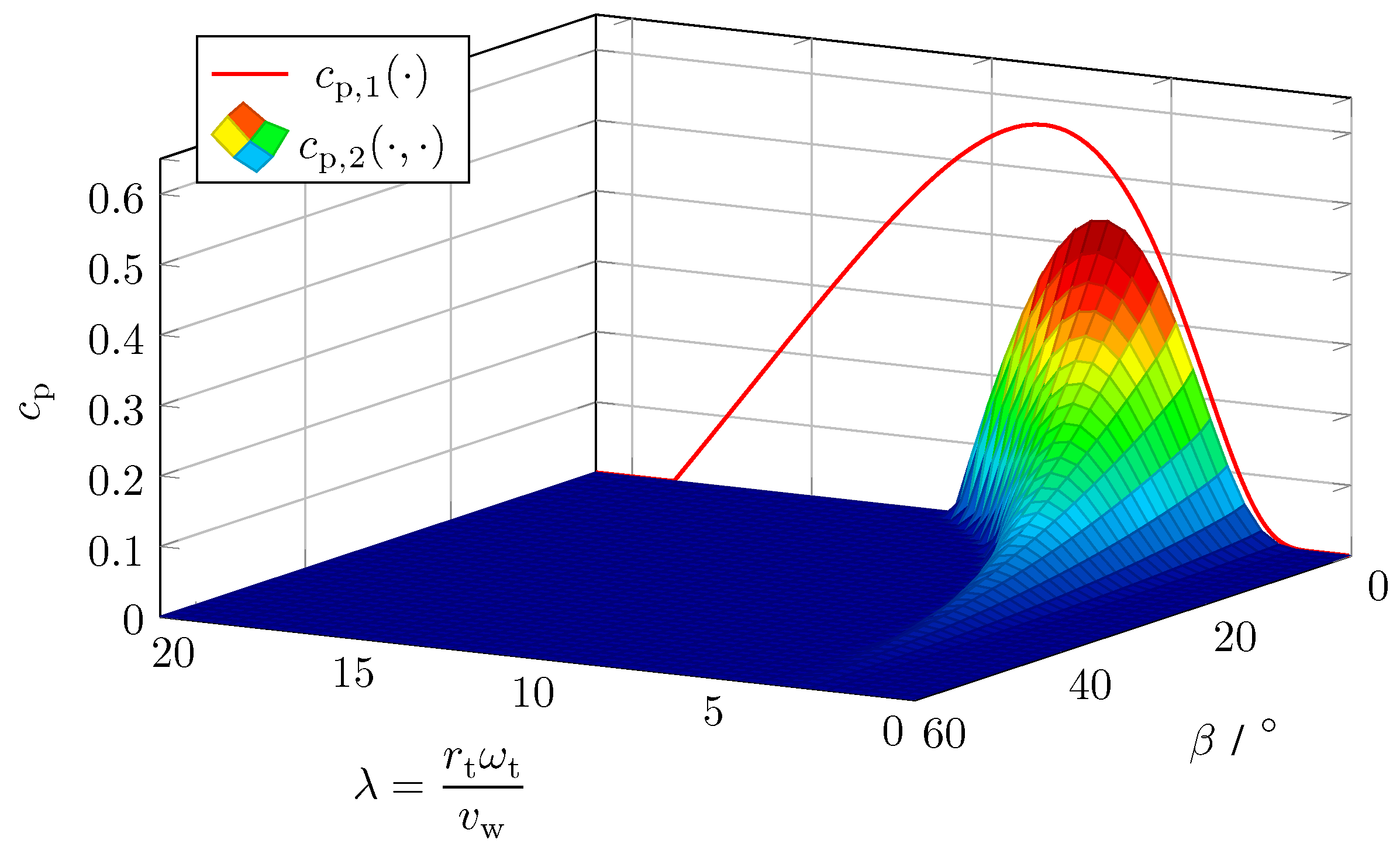
- Power coefficient without pitch control system (i.e., ) :which has a global maximum at with .
- Power coefficient with pitch control system (i.e., ):which, for , has its maximum at with .
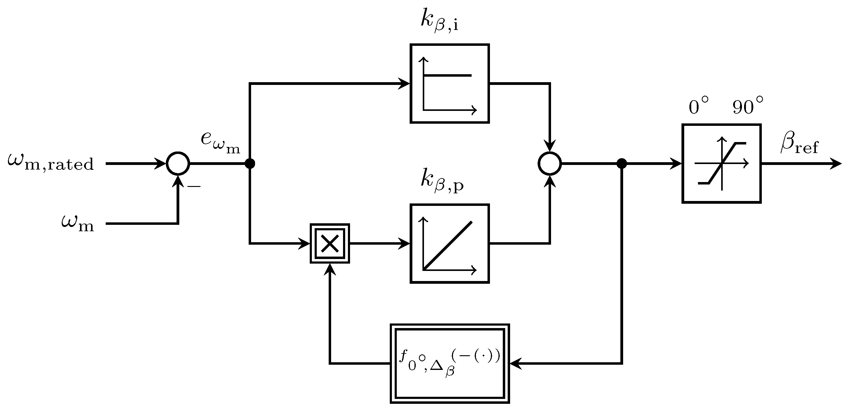
3.1.2. Pitch Control System
3.1.3. Turbine Torque
3.1.4. Drive Train
3.2. Electrical System in Three-Phase -Reference Frame
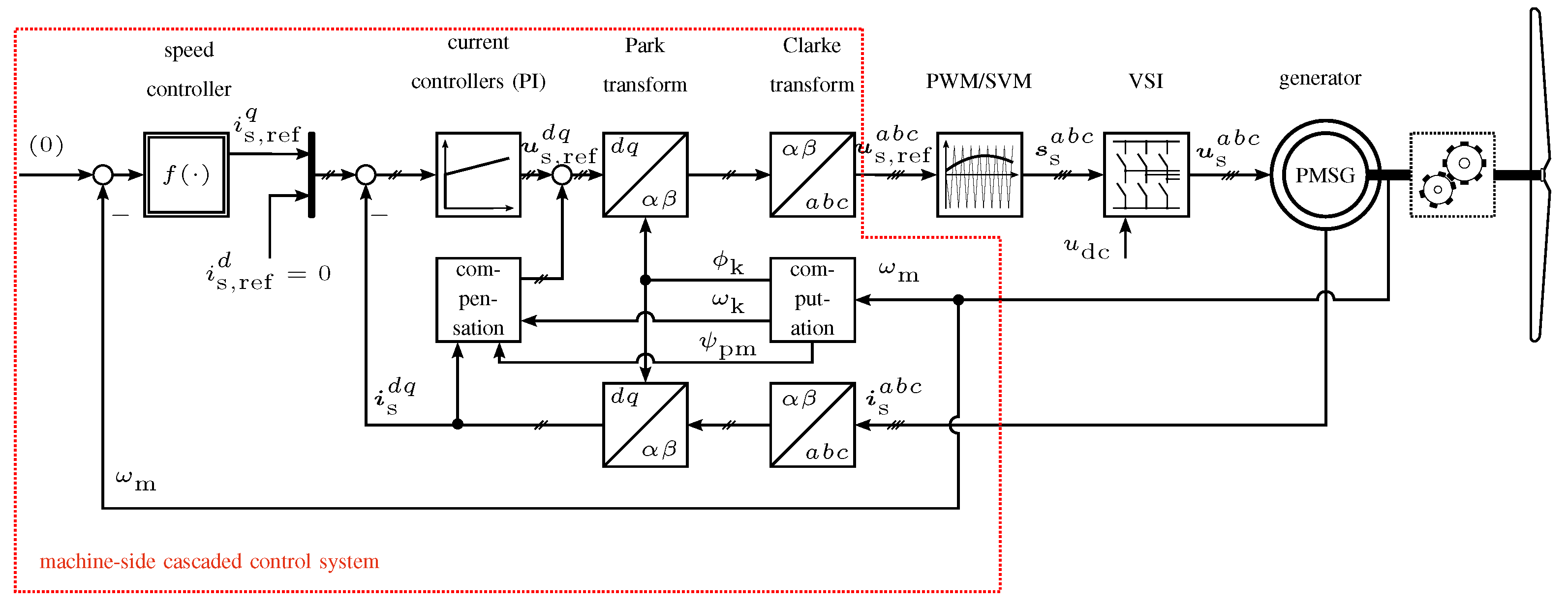
3.2.1. Machine-sIde Dynamics (Electrical Machine/Generator and Drive Train)
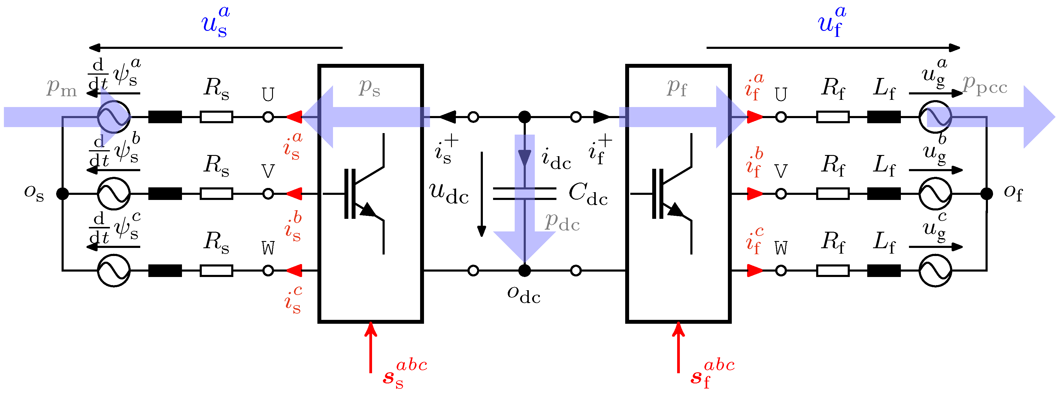
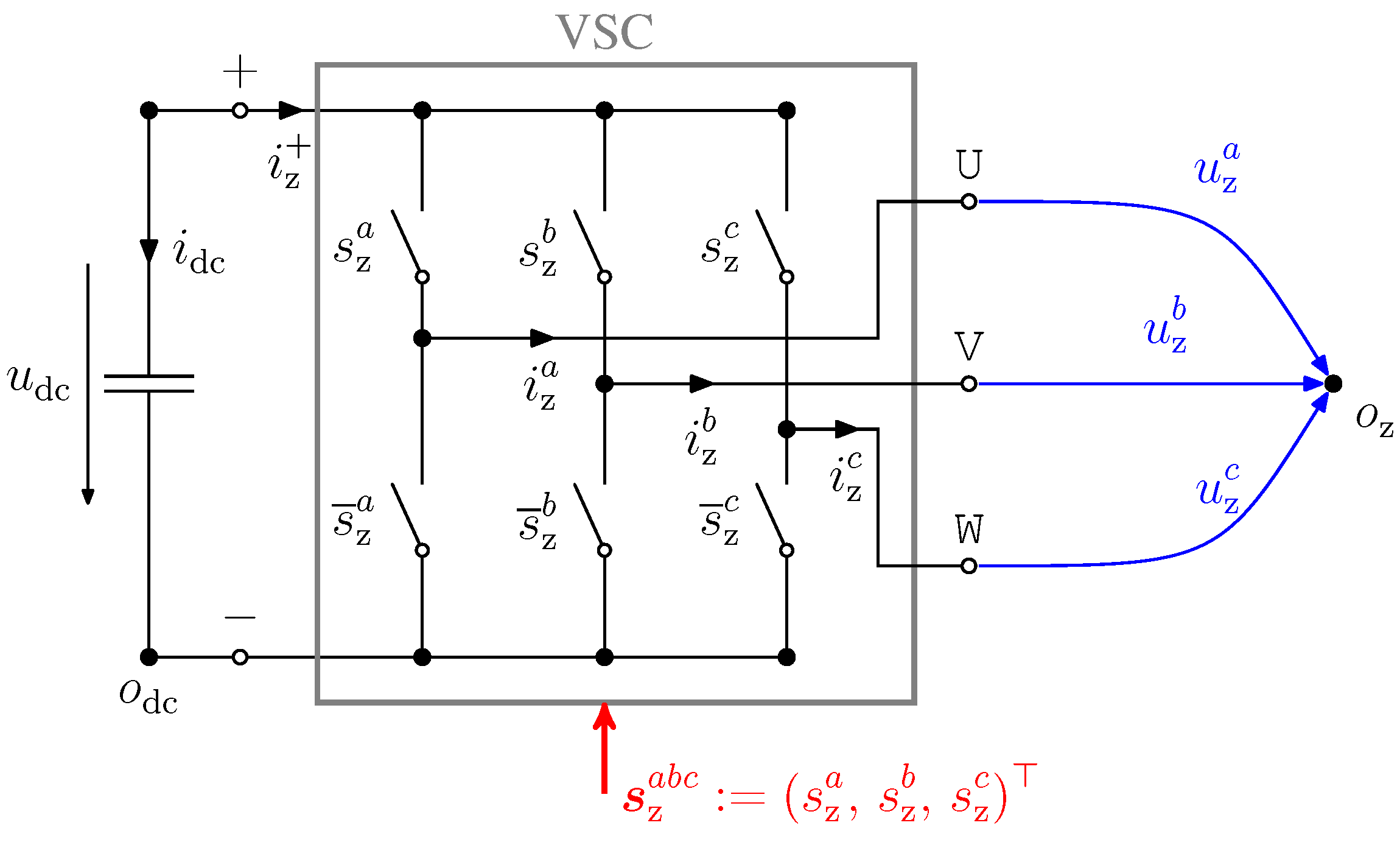
3.2.2. Power Electronics and DC-Link Dynamics (back-to-back Converter)
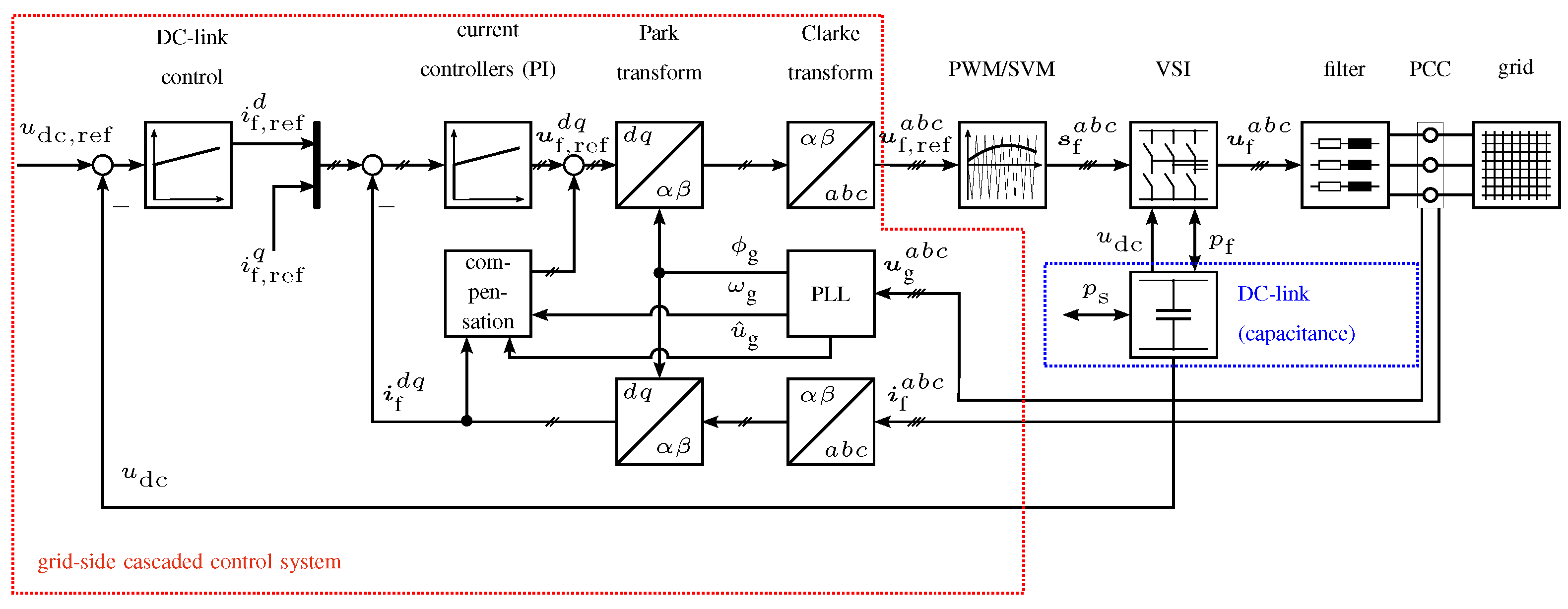
3.2.3. Grid-Side Dynamics (Filter, PCC and Grid)
3.2.4. Power Output
3.2.5. Overall Dynamics in Nonlinear State-Space Representation
3.3. Electrical System in (Simplified) Synchronously Rotating -Reference Frame
3.3.1. Machine-Side Dynamics: Electrical Machine (Generator) and Drive Train
3.3.2. Power Electronics and DC-Link Dynamics (Back-to-Back Converter)
3.3.3. Grid-Side Dynamics (Filter, PCC, and Grid)
3.3.4. Power Output
3.3.5. Overall Dynamics in Nonlinear State-Space Representation
4. Control Systems and Operation Management
4.1. Controllers
4.1.1. Machine-Side and Grid-Side Current Controllers ()
4.1.2. Speed Controller (Regime II)
4.1.3. Torque Controller and Pitch Reference Controller (Regime III)
4.1.4. DC-Link Voltage Controller and Reactive Power Feedforward Controller
4.2. Operation Management
5. Reduced-Order Models
5.1. Non-Switching Model (Nsm) or Averaging Model
5.2. Reduced-Order Model (ROM)
6. Implementation and Comparative Simulations
- Figure 10 compares DC-link voltage , mechanical angular velocity , pitch angle and tip speed ratio of all three models;
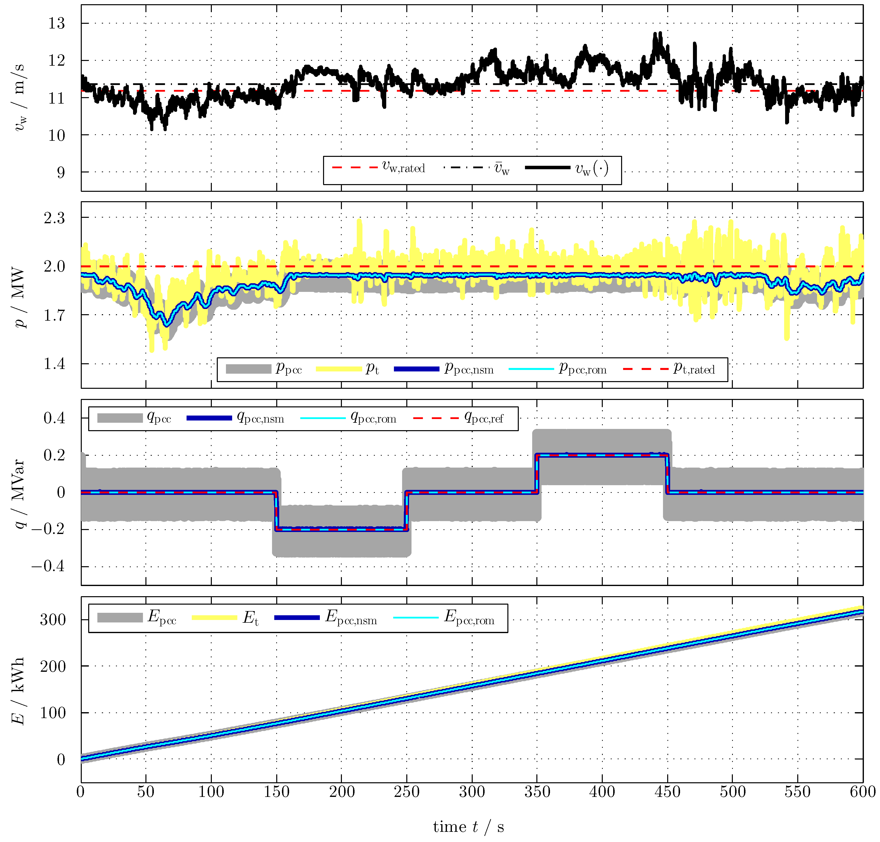
- Figure 11 compares turbine , active and reactive power (at the PCC) and the produced energy E of all three models; and
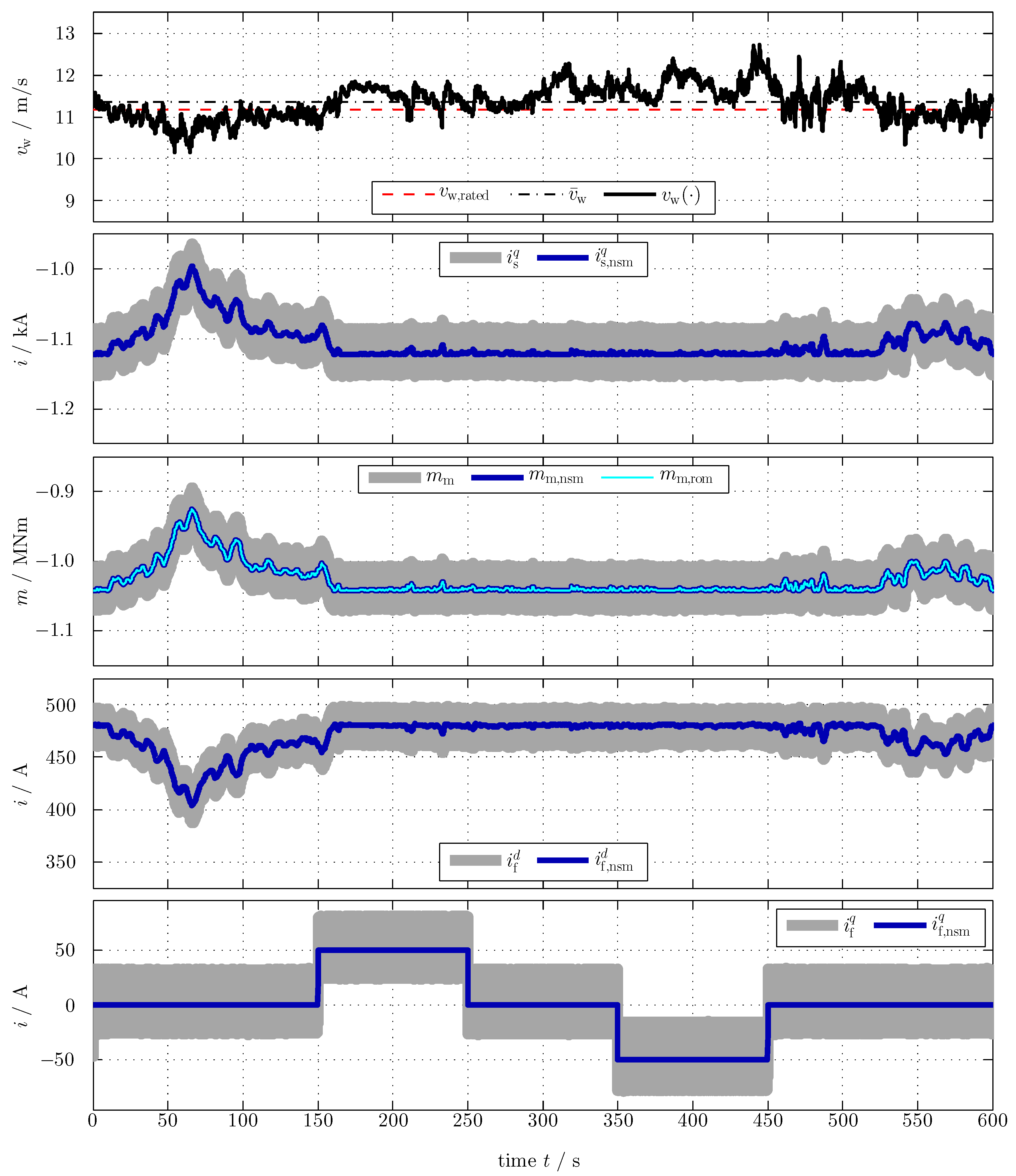
- Figure 12 compares machine torque of all three models and currents , , & of full-order model and non-switching model.
7. Conclusions
Author Contributions
Funding
Conflicts of Interest
Nomenclature
| Mathematical symbols and functions | |
| natural, real, complex numbers | |
| ; () | real numbers greater than (and equal to) |
| space of continuous functions mapping | |
| column vector with (where “” and “” mean “transposed” and “is defined as”, resp.) | |
| ; | zero; unity vector |
| scalar product of the vectors and | |
| (square) matrix with n rows and columns | |
| ; | inverse matrix; transposed inverse of (if exists). |
| ; | identity; zero matrix with |
x | saturation functions, for and , given by |
| transition function, for and , given by | |
| Reference frames and transformation/rotation matrices for modeling | |
| quantity vector in the three-phase -reference frame | |
| quantity vector in the synchronously rotating -reference frame | |
| ; | (reduced) Clarke-Park-transformation matrix; its inverse matrix, relating , and, for given by [60] (Appendix A.5) |
| ; | rotation matrices (counter-clock wise by ), given by |
| Physical quantitities | |
| ; ; ; ; | stator voltages; currents in or -reference frame; power |
| ; ; ; | stator resistance; main; mutual; leakage (stray) inductance |
| ; | stator inductance matrices in or -reference frame |
| ; ; ; | stator and permanent-magnet flux linkages in or -reference frame |
| ; ; ; | filter voltages; currents in or -reference frame; power |
| ; | filter resistance; inductance |
| ; ; ; ; | grid voltages in or -reference frame; voltage amplitude; angle; angular frequency |
| ; ; ; | DC-link voltage; current; power; capacitance |
| ; ; | switching vector for machine (stator); grid (filter); switching frequency |
| ; ; ; ; ; | turbine angular frequency; torque; radius; power; inertia; gear ratio |
| ; ; ; ; | wind speed; power; pitch angle; tip speed ratio; power coefficient |
| ; ; ; ; ; | machine (generator) angular position; angular frequency; torque; power; inertia; number of pole pairs |
| ; | active; reactive (instantaneous) power at point of common coupling (PCC) |
References
- Global Wind Energy Council. Global Wind Report 2017; Technical Report; GWEC: Brussels, Belgium, 2017. [Google Scholar]
- Park, G.L. Planning Manual for Utility Application of WECS. In Technical Report, Michigan State University, East Lansing (USA); Division of Engineering Research: Room, Italy, 1979. [Google Scholar]
- Øye, S. Unsteady Wake Effects Caused by Pitch-Angle Changes. In IEA R&D WECS Joint Action on Aerodynamics of Wind Turbines; IEA: Paris, France, 1986; pp. 58–79. [Google Scholar]
- Anderson, P.M.; Bose, A. Stability Simulation of Wind Turbine Systems. IEEE Trans. Power Appar. Syst. 1983, PAS-102, 3791–3795. [Google Scholar] [CrossRef]
- Petru, T.; Thiringer, T. Modeling of Wind Turbines for Power System Studies. IEEE Trans. Power Syst. 2002, 17, 1132–1139. [Google Scholar] [CrossRef]
- Papathanassiou, S.A.; Papadopoulos, M.P. Dynamic Behavior of Variable Speed Wind Turbines under Stochastic Wind. IEEE Trans. Energy Convers. 1999, 14, 1617–1623. [Google Scholar] [CrossRef]
- Wu, B.; Lang, Y.; Zargari, N.; Kouro, S. Power Conversion and Control of Wind Energy Systems; John Wiley & Sons: Hoboken, NJ, USA, 2011. [Google Scholar]
- Behnke, M.; Ellis, A.; Kazachkov, Y.; McCoy, T.; Muljadi, E.; Price, W.; Sanchez-Gasca, J. Development and Validation of WECC Variable Speed Wind Turbine Dynamic Models for Grid Integration Studies; Technical Report; National Renewable Energy Laboratory (NREL); U.S. Department of Energy: Washington, DC, USA, 2007.
- Kojabadi, H.M.; Chang, L.; Boutot, T. Development of a Novel Wind Turbine Simulator for Wind Energy Conversion Systems Using an Inverter-Controlled Induction Motor. IEEE Trans. Energy Convers. 2004, 19, 547–552. [Google Scholar] [CrossRef]
- Slootweg, J.G.; Polinder, H.; Kling, W.L. Dynamic Modelling of a Wind Turbine with Doubly Fed Induction Generator. In Proceedings of the Power Engineering Society Summer Meeting, Vancouver, BC, Canada, 15–19 July 2001; pp. 644–649. [Google Scholar]
- Miller, N.W.; Sanchez-Gasca, J.J.; Price, W.W.; Delmerico, R.W. Dynamic Modeling of GE 1.5 and 3.6 MW Wind Turbine-Generators for Stability Simulations. In Proceedings of the IEEE Power Engineering Society General Meeting, Toronto, ON, Canada, 13–17 July 2003; pp. 1977–1983. [Google Scholar]
- Ekanayake, J.B.; Holdsworth, L.; Wu, X.; Jenkins, N. Dynamic Modeling of Doubly Fed Induction Generator Wind Turbines. IEEE Trans. Power Syst. 2003, 18, 803–809. [Google Scholar] [CrossRef]
- Lei, Y.; Mullane, A.; Lightbody, G.; Yacamini, R. Modeling of the Wind Turbine with a Doubly Fed Induction Generator for Grid Integration Studies. IEEE Trans. Energy Convers. 2006, 21, 257–264. [Google Scholar] [CrossRef]
- Chowdhury, B.H.; Chellapilla, S. Double-Fed Induction Generator Control for Variable Speed Wind Power Generation. Electr. Power Syst. Res. 2006, 76, 786–800. [Google Scholar] [CrossRef]
- Sun, Z.; Wang, H.; Li, Y. Modelling and Simulation of Doubly-Fed Induction Wind Power System Based on Matlab/Simulink. In Proceedings of the International Conference on Sustainable Power Generation and Supply, Hangzhou, China, 8–9 September 2012. [Google Scholar]
- Subramanian, C.; Casadei, D.; Tani, A.; Rossi, C. Modeling and Simulation of Grid Connected Wind Energy Conversion System Based on a Doubly Fed Induction Generator (DFIG). Int. J. Electr. Energy 2014, 2. [Google Scholar] [CrossRef]
- Singh, M.; Santoso, S. Dynamic Models for Wind Turbines and Wind Power Plants; Technical Report, National Renewable Energy Laboratory (NREL); U.S. Department of Energy: Washington, DC, USA, 2011.
- Lalor, G.; Mullane, A.; O’Malley, M. Frequency control and wind turbine technologies. IEEE Trans. Power Syst. 2005, 20, 1905–1913. [Google Scholar] [CrossRef]
- Tobías-González, A.; Pena-Gallardo, R.; Morales-Saldana, J.; Gutiérrez-Urueta, G. Modeling of a Wind Turbine with a Permanent Magnet Synchronous Generator for Real Time Simulations. In Proceedings of the 2015 IEEE International Autumn Meeting on Power, Electronics and Computing, Ixtapa, Mexico, 4–6 November 2015; pp. 1–6. [Google Scholar]
- Singh, M.; Santoso, S. Dynamic Model for Full-Converter Wind Turbines Employing Permanent Magnet Alternators. In Proceedings of the IEEE Power and Energy Society General Meeting, Detroit, MI, USA, 24–29 July 2011. [Google Scholar]
- Yin, M.; Li, G.; Zhou, M.; Zhao, C. Modeling of the Wind Turbine with a Permanent Magnet Synchronous Generator for Integration. In Proceedings of the Power Engineering Society General Meeting, Tampa, FL, USA, 24–28 June 2007; pp. 1–6. [Google Scholar]
- Sanchez, J.A.; Veganzones, C.; Martinez, S.; Blazquez, F.; Herrero, N.; Wilhelmi, J.R. Dynamic Model of Wind Energy Conversion Systems with Variable Speed Synchronous Generator and Full-Size Power Converter for Large-Scale Power System Stability Studies. Renew. Energy 2008, 33, 1186–1198. [Google Scholar] [CrossRef]
- Rolan, A.; Luna, A.; Vazquez, G.; Aguilar, D.; Azevedo, G. Modeling of a Variable Speed Wind Turbine With a Permanent Magnet Synchronous Generator. In Proceedings of the IEEE International Symposium on Industrial Electronics, Seoul, South Korea, 5–8 July 2009; pp. 734–739. [Google Scholar]
- Elbeji, O.; Hamed, M.B.; Sbita, L. PMSG Wind Energy Conversion System: Modeling and Control. Int. J. Mod. Nonlinear Theory Appl. 2014, 3, 88–97. [Google Scholar] [CrossRef]
- Rekioua, D. Wind Energy Conversion and Power Electronics Modeling. In Wind Power Electric System: Modeling, Simulation and Control; Springer: Berlin, Germany, 2014; pp. 51–76. [Google Scholar]
- Munteanu, I.; Bratcu, A.I.; Cutululis, N.A.; Ceanga, E. Optimal Control of Wind Energy Systems; Springer: Berlin, Germany, 2008. [Google Scholar]
- Burton, T.; Sharpe, D.; Jenkins, N.; Bossanyi, E. Wind Energy Handbook; John Wiley & Sons: Hoboken, NJ, USA, 2001. [Google Scholar]
- Schlipf, D.; Schlipf, D.; Kühn, M. Nonlinear model predictive control of wind turbines using LIDAR. Wind Energy 2012, 16, 1107–1129. [Google Scholar] [CrossRef]
- Zribi, M.; Alrifai, M.; Rayan, M. Sliding Mode Control of a Variable-Speed Wind Energy Conversion System Using a Squirrel Cage Induction Generator. Energies 2017, 10, 604. [Google Scholar] [CrossRef]
- Soliman, M.; Malik, O.P.; Westwick, D.T. Multiple Model Predictive Control for Wind Turbines with Doubly Fed Induction Generators. IEEE Trans. Sustain. Energy 2011, 2, 215–225. [Google Scholar] [CrossRef]
- Bououden, S.; Chadli, M.; Filali, S.; El Hajjaji, A. Fuzzy Model Based Multivariable Predictive Control of a Variable Speed Wind Turbine: LMI Approach. Renew. Energy 2012, 37, 434–439. [Google Scholar] [CrossRef]
- Rocha, R.; Martins Filho, L.S.M.; Bortolus, M.V. Optimal Multivariable Control for Wind Energy Conversion System—A Comparison Between H2 and H∞ Controllers. In Proceedings of the Conference on Decision and Control and the European Control Conference, Seville, Spain, 15 December 2005; pp. 7906–7911. [Google Scholar]
- Henriksen, L.C.; Poulsen, N.K.; Hansen, M.H. Nonlinear Model Predictive Control of a Simplified Wind Turbine. In IFAC World Congress; Elsevier: New York, NY, USA, 2011; pp. 551–556. [Google Scholar]
- Liu, X.; Kong, X. Nonlinear Model Predictive Control for DFIG-Based Wind Power Generation. IEEE Trans. Autom. Sci. Eng. 2014, 11, 1046–1055. [Google Scholar] [CrossRef]
- Yaramasu, V.; Wu, B.; Rivera, M.; Rodriguez, J. A New Power Conversion System for Megawatt PMSG Wind Turbines Using Four-Level Converters and a Simple Control Scheme Based on Two-Step Model Predictive Strategy—Part I: Modeling and Theoretical Analysis. IEEE J. Emerg. Sel. Top. Power Electron. 2014, 2, 3–13. [Google Scholar] [CrossRef]
- Lin, W.M.; Hong, C.M.; Ou, T.C.; Chiu, T.M. Hybrid intelligent control of PMSG wind generation system using pitch angle control with RBFN. Energy Convers. Manag. 2011, 52, 1244–1251. [Google Scholar] [CrossRef]
- Ou, T.C.; Lu, K.H.; Huang, C.J. Improvement of Transient Stability in a Hybrid Power Multi-System Using a Designed NIDC (Novel Intelligent Damping Controller). Energies 2017, 10, 488. [Google Scholar] [CrossRef]
- Zhang, Z.; Li, Z.; GAE, M.P.K.; Rodriguez, J.; GAE, R.K. Robust Predictive Control of Three-Level NPC Back-to-Back Converter PMSG Wind Turbine Systems with Revised Predictions. IEEE Trans. Power Electron. 2018, 1. [Google Scholar] [CrossRef]
- Arani, M.F.M.; Mohamed, Y.A.R.I. Assessment and Enhancement of a Full-Scale PMSG-Based Wind Power Generator Performance Under Faults. IEEE Trans. Energy Convers. 2016, 31, 728–739. [Google Scholar] [CrossRef]
- Shahriari, S.A.A.; Raoofat, M.; Dehghani, M.; Mohammadi, M.; Saad, M. Dynamic state estimation of a permanent magnet synchronous generator-based wind turbine. IET Renew. Power Gener. 2016, 10, 1278–1286. [Google Scholar] [CrossRef]
- Yu, S.; Emami, K.; Fernando, T.; Iu, H.H.C.; Wong, K.P. State estimation of doubly fed induction generator wind turbine in complex power systems. IEEE Trans. Power Syst. 2016, 31, 4935–4944. [Google Scholar] [CrossRef]
- Huerta, F.; Tello, R.L.; Prodanovic, M. Real-Time Power-Hardware-in-the-Loop Implementation of Variable-Speed Wind Turbines. IEEE Trans. Ind. Electron. 2017, 64, 1893–1904. [Google Scholar] [CrossRef]
- Bianchi, F.D.; Mantz, R.J.; De Battista, H. Modelling of Variable-Speed Variable-Pitch Wind Energy Conversion Systems. In Wind Turbine Control Systems: Principles, Modelling and Gain Scheduling Design; Springer: Berlin, Germany, 2007; pp. 29–48. [Google Scholar]
- Schubert, M. Verfahren Zur Regelung Einer Windenergieanlage und Windenergieanlage mit Einem Rotor. Germany Patent DE102004054608B4, 29 June 2006. [Google Scholar]
- Dirscherl, C.; Hackl, C.; Schechner, K. Modellierung und Regelung von modernen Windkraftanlagen: Eine Einführung (see https://arxiv.org/abs/1703.08661 for the English translation). In Elektrische Antriebe—Regelung von Antriebssystemen; Schröder, D., Ed.; Springer: Berlin, Germany, 2015; Chapter 24; pp. 1540–1614. [Google Scholar]
- Betz, A. Wind-Energie und ihre Ausnutzung durch Windmühlen; Vandenhoeck & Ruprecht: Göttingen, Germany, 1926. [Google Scholar]
- Heier, S. Windkraftanlagen: Systemauslegung, Netzintegration und Regelung, 5th ed.; Springer Vieweg+Teubner Verlag: Berlin, Germany, 2009. [Google Scholar]
- Hackl, C.M. Non-identifier based adaptive control in mechatronics: Theory and Application; Number 466 in Lecture Notes in Control and Information Sciences; Springer International Publishing: Berlin, Germany, 2017. [Google Scholar] [CrossRef]
- Koch, F.W. Simulation und Analyse der Dynamischen Wechselwirkung von Windenergieanlagen mit dem Elektroenergiesystem. Ph.D. Thesis, Universität Duisburg-Essen, Duisburg, Germany, 2005. [Google Scholar]
- Slootweg, J.; De Haan, S.W.H.; Polinder, H.; Kling, W. General model for representing variable speed wind turbines in power system dynamics simulations. IEEE Trans. Power Syst. 2003, 18, 144–151. [Google Scholar] [CrossRef]
- Slootweg, J.G.; Polinder, H.; Kling, W.L. Initialization of wind turbine models in power system dynamics simulations. In Proceedings of the 2001 IEEE Porto Power Tech Proceedings (Cat. No.01EX502), Porto, Portugal, 10–13 September 2001; Volume 4, p. 6. [Google Scholar] [CrossRef]
- Eldeeb, H.; Hackl, C.M.; Kullick, J. Efficient operation of anisotropic synchronous machines for wind energy systems. In Proceedings of the 6th Edition of the Conference “The Science of Making Torque from Wind” (TORQUE 2016), Munich, Germany, 5–7 October 2016; Volume 753. [Google Scholar] [CrossRef]
- Blaabjerg, F.; Liserre, M.; Ma, K. Power Electronics Converters for Wind Turbine Systems. IEEE Trans. Ind. Appl. 2012, 48, 708–718. [Google Scholar] [CrossRef]
- Schröder, D. Leistungselektronische Schaltungen: Funktion, Auslegung und Anwendung; Springer: Berlin, Germany, 2012. [Google Scholar]
- Bernet, S. Selbstgeführte Stromrichter am Gleichspannungszwischenkreis: Funktion, Modulation und Regelung; Springer: Berlin, Germany, 2012. [Google Scholar]
- Holmes, D.G.; Lipo, T.A. Pulse Width Modulation For Power Converters; IEEE Series on Power Engineering; IEEE Press: Piscataway, NJ, USA, 2003. [Google Scholar]
- Schröder, D. Leistungselektronische Schaltungen—Funktion, Auslegung und Anwendung (2. Auflage); Springer: Berlin, Germany, 2008. [Google Scholar]
- Böcker, J.; Beineke, S.; Bähr, A. On the Control Bandwidth of Servo Drives. In Proceedings of the 13th European Conference on Power Electronics and Applications, Barcelona, Spain, 8–10 September 2009; pp. 1–10. [Google Scholar]
- DIN Deutsches Institut für Normung e. V. DIN EN 50160:2011-02: Merkmale der Spannung in öffentlichen Elektrizitätsversorgungsnetzen; Norm 2011-02; Beuth Verlag: Berlin, Germany, 2011. [Google Scholar]
- Teodorescu, R.; Liserre, M.; Rodriguez, P. Grid Converters for Photovoltaic and Wind Power Systems; John Wiley & Sons, Ltd.: Chichester, UK, 2011. [Google Scholar]
- Dirscherl, C.; Fessler, J.; Hackl, C.M.; Ipach, H. State-feedback controller and observer design for grid-connected voltage source power converters with LCL-filter. In Proceedings of the 2015 IEEE International Conference on Control Applications (CCA), Sydney, NSW, Australia, 21–23 September 2015; pp. 215–222. [Google Scholar] [CrossRef]
- Hackl, C.M. MPC with analytical solution and integral error feedback for LTI MIMO systems and its application to current control of grid-connected power converters with LCL-filter. In Proceedings of the 2015 IEEE International Symposium on Predictive Control of Electrical Drives and Power Electronics (PRECEDE), Valparaiso, Chile, 5–6 October 2015; pp. 61–66. [Google Scholar] [CrossRef]
- Schröder, D. Elektrische Antriebe—Regelung von Antriebssystemen (3., Bearb. Auflage); Springer: Berlin, Germany, 2009. [Google Scholar]
- Hackl, C.M. On the equivalence of proportional-integral and proportional-resonant controllers with anti-windup. arXiv 2016, arXiv:1610.07133. [Google Scholar]
- Åström, K.J.; Rundqwist, L. Integrator windup and how to avoid it. In Proceedings of the American Control Conference, Pittsburgh, PA, USA, 21–23 June 1989; pp. 1693–1698. [Google Scholar]
- Peng, Y.; Vranic, D.; Hanus, R. Anti-windup, bumpless, and conditioned transfer techniques for PID controllers. IEEE Control Syst. Mag. 1996, 16, 48–57. [Google Scholar] [CrossRef]
- Kessler, G. Über die Vorausberechnung optimal abgestimmter Regelkreise—Teil 3: Die optimale Einstellung des Reglers nach dem Betragsoptimum. Regelungstechnik 1955, 3, 40–49. [Google Scholar]
- Hackl, C.; Schechner, K. Non-ideal feedforward torque control of wind turbines: Impacts on annual energy production & gross earnings. J. Phys. 2016, 753, 112010. [Google Scholar]
- Mullen, J.; Hoagg, J.B. Wind Turbine Torque Control for Unsteady Wind Speeds Using Approximate-Angular-Acceleration Feedback. In Proceedings of the 52nd IEEE Conference on Decision and Control (CDC), Florence, Italy, 10–13 December 2013; pp. 397–402. [Google Scholar]
- Dirscherl, C.; Hackl, C.M.; Schechner, K. Pole-placement based nonlinear state-feedback control of the DC-link voltage in grid-connected voltage source power converters: A preliminary study. In Proceedings of the 2015 IEEE International Conference on Control Applications (CCA) (CCA), Sydney, NSW, Australia, 21–23 September 2015; pp. 207–214. [Google Scholar] [CrossRef]
- Schechner, K.; Bauer, F.; Hackl, C.M. Nonlinear DC-link PI control for airborne wind energy systems during pumping mode. In Airborne Wind Energy: Advances in Technology Development and Research; Schmehl, R., Ed.; Springer: Berlin, Germany, 2016. [Google Scholar]
- Lescher, F.; Zhao, J.Y.; Borne, P. Switching LPV Controllers for a Variable Speed Pitch Regulated Wind Turbine. In Proceedings of the IMACS Multiconference on Computational Engineering in Systems Applications, Beijing, China, 4–6 October 2006; pp. 1334–1340. [Google Scholar]
- Duindam, V.; Macchelli, A.; Stramigioli, S.; Bruyninckx, H. (Eds.) Modeling and Control of Complex Physical Systems: The Port-Hamiltonian Approach; Springer: Berlin/Heidelberg, Germany, 2009. [Google Scholar]


| Description | Symbol | Value |
|---|---|---|
| Turbine & gear (direct drive) | ||
| Air density | ||
| Turbine radius | ||
| Turbine inertia | 8.6 × | |
| Power coefficient | as in (4) | |
| Maximal change rate of pitch angle | ||
| Pitch control time constant | ||
| Gear ratio | ||
| Permanent magnet synchronous generator (isotropic) | ||
| Number of pole pairs | 48 | |
| Stator resistance | ||
| Stator inductance(s) | ||
| Permanent magnet flux | ||
| Generator inertia | 1.3 × | |
| Back-to-back converter | ||
| DC-link capacitance | ||
| Switching frequency | ||
| Delay | ||
| Filter & grid voltage | ||
| Filter resistance | ||
| Filter inductance | ||
| Grid angular frequency | ||
| Grid voltage amplitude | ||
| Grid voltage initial angle | ||
| Controller parameters | ||
| PI current controller (33) | ||
| (grid-side) | ||
| 1 × | ||
| PI current controller (33) | ||
| (machine-side) | ||
| 1 × | ||
| Speed controller (34) | ||
| DC-link voltage | ||
| PI controller (36) | ||
| Phased-locked loop | ||
| PI controller as in [45] | ||
| Pitch angle reference | ||
| PI controller (35) | ||
| 1 × | ||
| Full-Order Model (29) | Non-Switching Model (40) | Reduced-Order Model (47) | |
|---|---|---|---|
| order | 9 | 7 | 3 |
| OS | Windows 10 | Windows 10 | Windows 10 |
| (Education 64-bit) | (Education 64-bit) | (Education 64-bit) | |
| CPU | Intel Xenon E5-1650 v3 | Intel Xenon E5-1650 v3 | Intel Xenon E5-1650 v3 |
| (3.50 GHz, 12 CPUs) | (3.50 GHz, 12 CPUs) | (3.50 GHz, 12 CPUs) | |
| RAM | 131,072 MB | 131,072 MB | 131,072 MB |
| Software | Matlab Simulink | Matlab Simulink | Matlab Simulink |
| (R2013b 64-bit) | (R2016a 64-bit) | (R2016a 64-bit) | |
| Step size | 4 × | 2 × | 2 × |
| Solver | Runge-Kutta (ode4) | Runge-Kutta (ode4) | Runge-Kutta (ode4) |
| Duration | 10,680 s (2:58 h) | 16 | 11 |
© 2018 by the authors. Licensee MDPI, Basel, Switzerland. This article is an open access article distributed under the terms and conditions of the Creative Commons Attribution (CC BY) license (http://creativecommons.org/licenses/by/4.0/).
Share and Cite
Hackl, C.M.; Jané-Soneira, P.; Pfeifer, M.; Schechner, K.; Hohmann, S. Full- and Reduced-Order State-Space Modeling of Wind Turbine Systems with Permanent Magnet Synchronous Generator. Energies 2018, 11, 1809. https://doi.org/10.3390/en11071809
Hackl CM, Jané-Soneira P, Pfeifer M, Schechner K, Hohmann S. Full- and Reduced-Order State-Space Modeling of Wind Turbine Systems with Permanent Magnet Synchronous Generator. Energies. 2018; 11(7):1809. https://doi.org/10.3390/en11071809
Chicago/Turabian StyleHackl, Christoph M., Pol Jané-Soneira, Martin Pfeifer, Korbinian Schechner, and Sören Hohmann. 2018. "Full- and Reduced-Order State-Space Modeling of Wind Turbine Systems with Permanent Magnet Synchronous Generator" Energies 11, no. 7: 1809. https://doi.org/10.3390/en11071809
APA StyleHackl, C. M., Jané-Soneira, P., Pfeifer, M., Schechner, K., & Hohmann, S. (2018). Full- and Reduced-Order State-Space Modeling of Wind Turbine Systems with Permanent Magnet Synchronous Generator. Energies, 11(7), 1809. https://doi.org/10.3390/en11071809