Shadow Pricing of Electric Power Interruptions for Distribution System Operators in Finland


Abstract
:1. Introduction
2. Directional Distance Function and the Shadow Pricing of Electric Power Interruptions
- l: the constant of the quadratic directional distance function,
- αn: the input coefficients,
- βm: the desirable output coefficients,
- γj: the undesirable output coefficients,
- αmn′: the quadratic of input coefficients,
- βmm′: the quadratic of desirable output coefficients,
- γjj′: the quadratic of undesirable output coefficients,
- δnm: the product of the inputs and desirable outputs coefficients,
- ηnj: the product of the inputs and undesirable outputs coefficients,
- μmj: the coefficients of the product of the desirable and undesirable outputs.
3. Empirical Study and Results
3.1. Empirical Study
3.2. Results
4. Discussion
5. Conclusions
Author Contributions
Funding
Conflicts of Interest
Appendix A

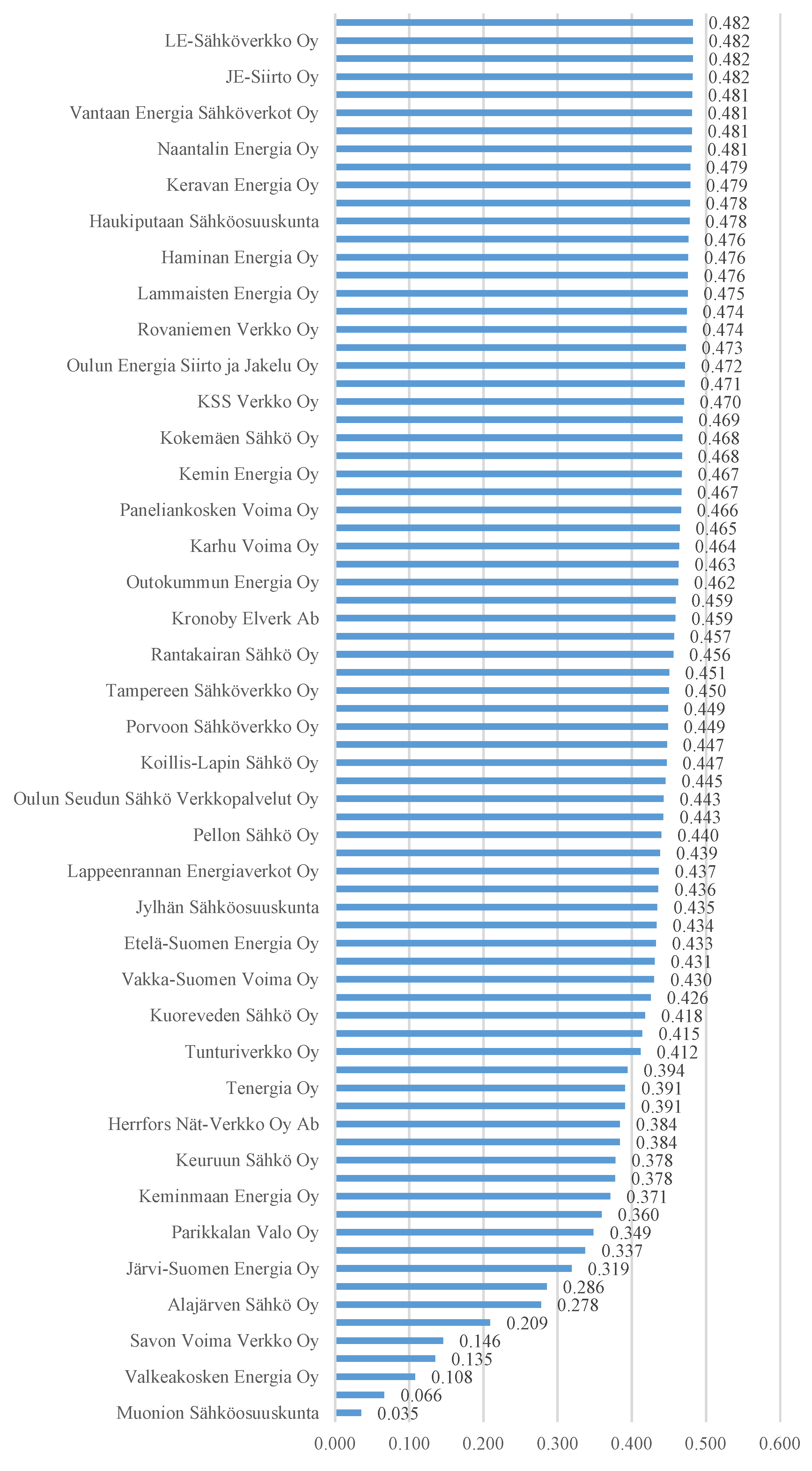
| DSO | 2013 | 2014 | 2015 | DSO | 2013 | 2014 | 2015 |
|---|---|---|---|---|---|---|---|
| Äänekosken Energia Oy | 0.454 | 0.449 | 0.457 | Lehtimäen Sähkö Oy | 0.457 | 0.461 | 0.443 |
| Alajärven Sähkö Oy | 0.447 | 0.466 | 0.278 | Leppäkosken Sähkö Oy | 0.457 | 0.470 | 0.468 |
| Caruna Espoo Oy | 0.462 | 0.472 | 0.474 | LE-Sähköverkko Oy | 0.477 | 0.481 | 0.482 |
| Caruna Oy | 0.348 | 0.447 | 0.439 | Mäntsälän Sähkö Oy | 0.458 | 0.474 | 0.467 |
| Ekenäs Energi Ab | 0.477 | 0.470 | 0.471 | Muonion Sähköosuuskunta | 0.426 | 0.343 | 0.035 |
| Elenia Oy | 0.295 | 0.445 | 0.209 | Naantalin Energia Oy | 0.479 | 0.479 | 0.481 |
| Enontekiön Sähkö Oy | 0.000 | 0.357 | 0.337 | Nurmijärven Sähköverkko Oy | 0.463 | 0.474 | 0.469 |
| ESE-Verkko Oy | 0.480 | 0.482 | 0.479 | Nykarleby Kraftverk Ab | 0.429 | 0.422 | 0.426 |
| Esse Elektro-Kraft Ab | 0.416 | 0.452 | 0.286 | Oulun Energia Siirto ja Jakelu Oy | 0.468 | 0.470 | 0.472 |
| Etelä-Suomen Energia Oy | 0.364 | 0.399 | 0.433 | Oulun Seudun S. Verkkopalvelut Oy | 0.452 | 0.467 | 0.443 |
| Forssan Verkkopalvelut Oy | 0.481 | 0.482 | 0.482 | Outokummun Energia Oy | 0.457 | 0.432 | 0.462 |
| Haminan Energia Oy | 0.478 | 0.480 | 0.476 | Paneliankosken Voima Oy | 0.414 | 0.472 | 0.466 |
| Haukiputaan Sähköosuuskunta | 0.471 | 0.474 | 0.478 | Parikkalan Valo Oy | 0.179 | 0.444 | 0.349 |
| Helen Sähköverkko Oy | 0.483 | 0.483 | 0.482 | Pellon Sähkö Oy | 0.465 | 0.449 | 0.440 |
| Herrfors Nät-Verkko Oy Ab | 0.347 | 0.433 | 0.384 | PKS Sähkönsiirto Oy | 0.376 | 0.376 | 0.066 |
| Iin Energia Oy | 0.477 | 0.478 | 0.459 | Pori Energia Sähköverkot Oy | 0.386 | 0.440 | 0.449 |
| Imatran Seudun Sähkönsiirto Oy | 0.268 | 0.448 | 0.394 | Porvoon Sähköverkko Oy | 0.399 | 0.439 | 0.449 |
| Järvi-Suomen Energia Oy | 0.242 | 0.438 | 0.319 | Raahen Energia Oy | 0.482 | 0.480 | 0.481 |
| Jeppo Kraft Andelslag | 0.454 | 0.453 | 0.445 | Rantakairan Sähkö Oy | 0.465 | 0.466 | 0.456 |
| JE-Siirto Oy | 0.481 | 0.480 | 0.482 | Rauman Energia Oy | 0.445 | 0.475 | 0.463 |
| Jylhän Sähköosuuskunta | 0.457 | 0.474 | 0.435 | Rovakaira Oy | 0.413 | 0.452 | 0.431 |
| Karhu Voima Oy | 0.481 | 0.477 | 0.464 | Rovaniemen Verkko Oy | 0.480 | 0.480 | 0.474 |
| Kemin Energia Oy | 0.478 | 0.479 | 0.467 | Sallila Sähkönsiirto Oy | 0.434 | 0.466 | 0.465 |
| Keminmaan Energia Oy | 0.446 | 0.478 | 0.371 | Savon Voima Verkko Oy | 0.175 | 0.287 | 0.146 |
| KENET Oy | 0.469 | 0.473 | 0.476 | Seiverkot Oy | 0.470 | 0.475 | 0.476 |
| Keravan Energia Oy | 0.472 | 0.468 | 0.479 | Tampereen Sähköverkko Oy | 0.449 | 0.478 | 0.450 |
| Keuruun Sähkö Oy | 0.355 | 0.414 | 0.378 | Tenergia Oy | 0.405 | 0.427 | 0.391 |
| Koillis-Lapin Sähkö Oy | 0.371 | 0.445 | 0.447 | Tornion Energia Oy | 0.469 | 0.473 | 0.447 |
| Koillis-Satakunnan Sähkö Oy | 0.441 | 0.443 | 0.415 | Tornionlaakson Sähkö Oy | 0.418 | 0.463 | 0.436 |
| Kokemäen Sähkö Oy | 0.425 | 0.466 | 0.468 | Tunturiverkko Oy | 0.443 | 0.451 | 0.412 |
| Köyliön-Säkylän Sähkö Oy | 0.452 | 0.469 | 0.473 | Turku Energia Sähköverkot Oy | 0.469 | 0.481 | 0.481 |
| Kronoby Elverk Ab | 0.440 | 0.410 | 0.459 | Vaasan Sähköverkko Oy | 0.417 | 0.430 | 0.434 |
| KSS Verkko Oy | 0.454 | 0.455 | 0.470 | Vakka-Suomen Voima Oy | 0.352 | 0.458 | 0.430 |
| Kuopion Sähköverkko Oy | 0.481 | 0.481 | 0.478 | Valkeakosken Energia Oy | 0.476 | 0.476 | 0.108 |
| Kuoreveden Sähkö Oy | 0.445 | 0.468 | 0.418 | Vantaan Energia Sähköverkot Oy | 0.479 | 0.480 | 0.481 |
| Kymenlaakson Sähköverkko Oy | 0.375 | 0.426 | 0.391 | Vatajankosken Sähkö Oy | 0.419 | 0.455 | 0.451 |
| Lammaisten Energia Oy | 0.457 | 0.473 | 0.475 | Verkko Korpela Oy | 0.323 | 0.253 | 0.378 |
| Lankosken Sähkö Oy | 0.274 | 0.410 | 0.384 | Vetelin Sähkölaitos Oy | 0.431 | 0.474 | 0.135 |
| Lappeenrannan Energiaverkot Oy | 0.401 | 0.455 | 0.437 | Vimpelin Voima Oy | 0.359 | 0.446 | 0.360 |
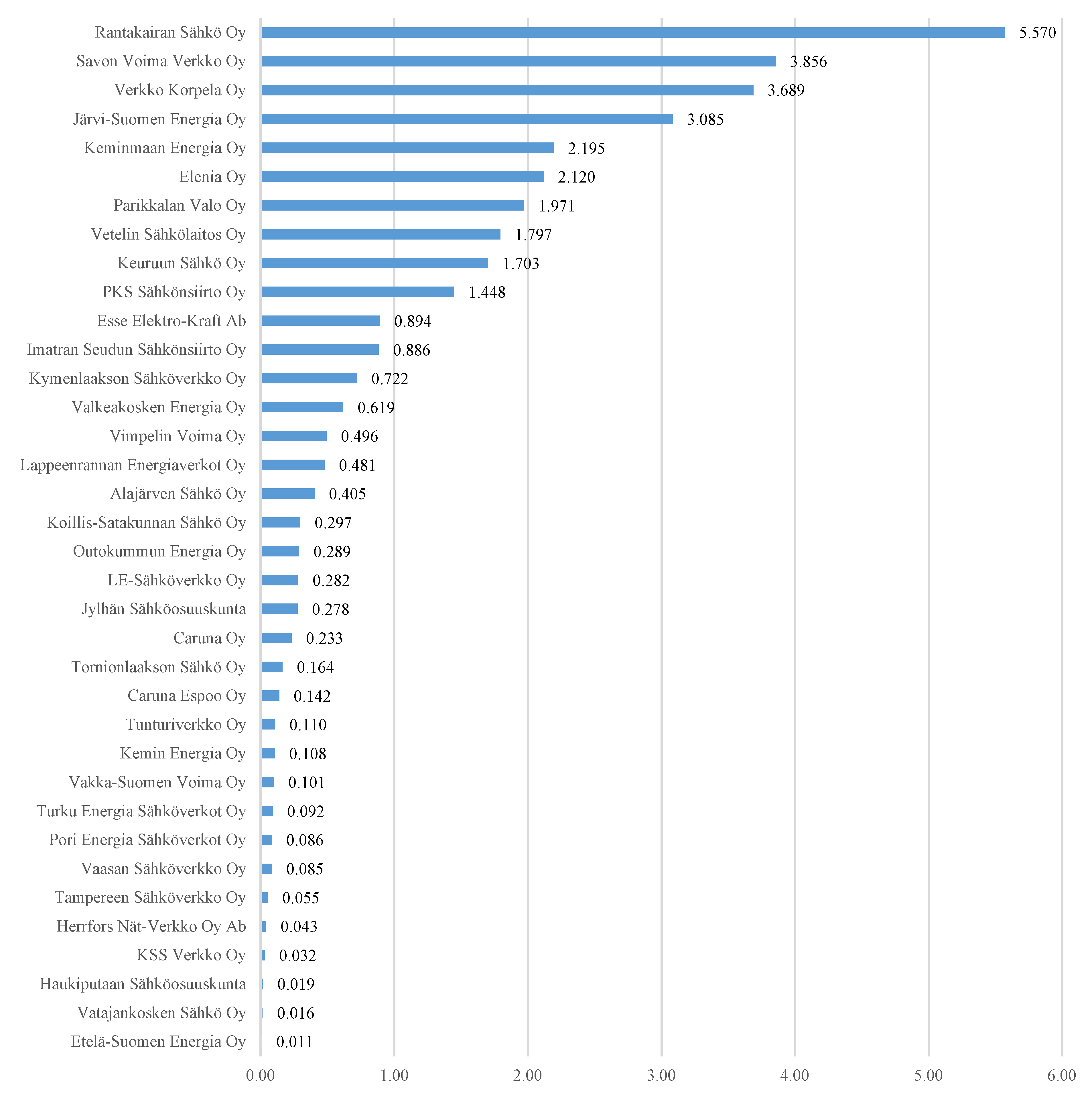
| DSO | 2013 | 2014 | 2015 | DSO | 2013 | 2014 | 2015 |
|---|---|---|---|---|---|---|---|
| Äänekosken Energia Oy | 1.87 | 2.20 | 1.68 | Lehtimäen Sähkö Oy | 1.66 | 1.44 | 2.57 |
| Alajärven Sähkö Oy | 2.29 | 1.10 | 13.29 | Leppäkosken Sähkö Oy | 1.67 | 0.87 | 1.02 |
| Caruna Espoo Oy | 1.37 | 0.74 | 0.60 | LE-Sähköverkko Oy | 0.42 | 0.17 | 0.11 |
| Caruna Oy | 8.69 | 2.30 | 2.85 | Mäntsälän Sähkö Oy | 1.62 | 0.65 | 1.07 |
| Ekenäs Energi Ab | 0.41 | 0.85 | 0.80 | Muonion Sähköosuuskunta | 3.35 | 9.00 | 30.21 |
| Elenia Oy | 12.16 | 2.41 | 17.93 | Naantalin Energia Oy | 0.32 | 0.29 | 0.20 |
| Enontekiön Sähkö Oy | 32.80 | 8.10 | 9.35 | Nurmijärven Sähköverkko Oy | 1.32 | 0.60 | 0.96 |
| ESE-Verkko Oy | 0.22 | 0.09 | 0.31 | Nykarleby Kraftverk Ab | 3.46 | 3.91 | 3.65 |
| Esse Elektro-Kraft Ab | 4.31 | 2.01 | 12.78 | Oulun Energia Siirto ja Jakelu Oy | 0.98 | 0.84 | 0.76 |
| Etelä-Suomen Energia Oy | 7.62 | 5.39 | 3.22 | Oulun Seudun S. Verkkopalvelut Oy | 1.99 | 1.05 | 2.56 |
| Forssan Verkkopalvelut Oy | 0.19 | 0.09 | 0.10 | Outokummun Energia Oy | 1.69 | 3.25 | 1.34 |
| Haminan Energia Oy | 0.35 | 0.27 | 0.49 | Paneliankosken Voima Oy | 4.38 | 0.73 | 1.10 |
| Haukiputaan Sähköosuuskunta | 0.82 | 0.59 | 0.38 | Parikkalan Valo Oy | 19.99 | 2.49 | 8.62 |
| Helen Sähköverkko Oy | 0.08 | 0.06 | 0.11 | Pellon Sähkö Oy | 1.18 | 2.18 | 2.74 |
| Herrfors Nät-Verkko Oy Ab | 8.71 | 3.22 | 6.31 | PKS Sähkönsiirto Oy | 6.86 | 6.85 | 27.96 |
| Iin Energia Oy | 0.44 | 0.40 | 1.56 | Pori Energia Sähköverkot Oy | 6.22 | 2.76 | 2.20 |
| Imatran Seudun Sähkönsiirto Oy | 13.98 | 2.26 | 5.67 | Porvoon Sähköverkko Oy | 5.38 | 2.80 | 2.21 |
| Järvi-Suomen Energia Oy | 15.73 | 2.87 | 10.54 | Raahen Energia Oy | 0.12 | 0.27 | 0.18 |
| Jeppo Kraft Andelslag | 1.90 | 1.95 | 2.41 | Rantakairan Sähkö Oy | 1.16 | 1.11 | 1.74 |
| JE-Siirto Oy | 0.20 | 0.26 | 0.13 | Rauman Energia Oy | 2.44 | 0.55 | 1.30 |
| Jylhän Sähköosuuskunta | 1.67 | 0.59 | 3.09 | Rovakaira Oy | 4.44 | 2.00 | 3.33 |
| Karhu Voima Oy | 0.19 | 0.40 | 1.24 | Rovaniemen Verkko Oy | 0.22 | 0.24 | 0.63 |
| Kemin Energia Oy | 0.39 | 0.33 | 1.03 | Sallila Sähkönsiirto Oy | 3.12 | 1.13 | 1.21 |
| Keminmaan Energia Oy | 2.36 | 0.37 | 7.16 | Savon Voima Verkko Oy | 20.28 | 12.66 | 22.32 |
| KENET Oy | 0.92 | 0.69 | 0.49 | Seiverkot Oy | 0.86 | 0.57 | 0.52 |
| Keravan Energia Oy | 0.73 | 0.97 | 0.32 | Tampereen Sähköverkko Oy | 2.17 | 0.37 | 2.12 |
| Keuruun Sähkö Oy | 8.20 | 4.38 | 6.71 | Tenergia Oy | 5.00 | 3.60 | 5.86 |
| Koillis-Lapin Sähkö Oy | 7.20 | 2.42 | 2.32 | Tornion Energia Oy | 0.95 | 0.68 | 2.29 |
| Koillis-Satakunnan Sähkö Oy | 2.71 | 2.59 | 4.37 | Tornionlaakson Sähkö Oy | 4.17 | 1.28 | 3.01 |
| Kokemäen Sähkö Oy | 3.68 | 1.15 | 1.00 | Tunturiverkko Oy | 2.57 | 2.08 | 4.52 |
| Köyliön-Säkylän Sähkö Oy | 1.99 | 0.91 | 0.69 | Turku Energia Sähköverkot Oy | 0.96 | 0.17 | 0.16 |
| Kronoby Elverk Ab | 2.77 | 4.69 | 1.57 | Vaasan Sähköverkko Oy | 4.24 | 3.40 | 3.17 |
| KSS Verkko Oy | 1.86 | 1.81 | 0.86 | Vakka-Suomen Voima Oy | 8.41 | 1.64 | 3.36 |
| Kuopion Sähköverkko Oy | 0.19 | 0.19 | 0.35 | Valkeakosken Energia Oy | 0.48 | 0.47 | 25.00 |
| Kuoreveden Sähkö Oy | 2.45 | 0.98 | 4.14 | Vantaan Energia Sähköverkot Oy | 0.31 | 0.27 | 0.17 |
| Kymenlaakson Sähköverkko Oy | 6.88 | 3.63 | 5.87 | Vatajankosken Sähkö Oy | 4.08 | 1.78 | 2.09 |
| Lammaisten Energia Oy | 1.67 | 0.67 | 0.53 | Verkko Korpela Oy | 10.33 | 14.93 | 6.73 |
| Lankosken Sähkö Oy | 13.56 | 4.67 | 6.31 | Vetelin Sähkölaitos Oy | 3.33 | 0.65 | 23.08 |
| Lappeenrannan Energiaverkot Oy | 5.27 | 1.78 | 2.96 | Vimpelin Voima Oy | 7.95 | 2.36 | 7.91 |
References
- Office of the Press Secretary. Presidential Policy Directive/Ppd-21, Critical Infrastructure Security and Resilience; The White House: Washington, DC, USA, 2013.
- Securing The U.S. Electrical Grid, Understanding the Threats to the Most Critical of Critical Infrastructure, While Securing a Changing Grid; Center for the Study of the Presidency & Congress: Washington, DC, USA, 2014.
- Küfeoğlu, S.; Prittinen, S.; Lehtonen, M. A summary of the recent extreme weather events and their impacts on electricity. Int. Rev. Electr. Eng. 2014, 9, 821–828. [Google Scholar] [CrossRef]
- Küfeoğlu, S.; Lehtonen, M. Interruption costs of service sector electricity customers, a hybrid approach. Int. J. Electr. Power Energy Syst. 2015, 64, 588–595. [Google Scholar] [CrossRef]
- Corwin, J.L.; Miles, W.T. Impact Assessment of the 1977 New York City Blackout; U.S. Department of Energy: Washington, DC, USA, 1978.
- Carlsson, F.; Martinsson, P.; Akay, A. The Effect of Power Outages and Cheap Talk on Willingness to Pay to Reduce Outages. Energy Econ. 2008, 30, 1232–1245. [Google Scholar] [CrossRef]
- Küfeoğlu, S.; Lehtonen, M. A Review on the Theory of Electric Power Reliability Worth and Customer Interruption Costs Assessment Techniques. In Proceedings of the 13th International Conference on the European Energy Market (EEM), Porto, Portugal, 6–9 June 2016. [Google Scholar]
- Sullivan, M.J.; Schellenberg, J.; Blundell, M. Updated Value of Service Reliability Estimates for Electric Utility Customers in the United States; Lawrence Berkeley National Laboratory: Berkeley, CA, USA, 2015.
- The Value of Lost Load (VoLL) for Electricity in Great Britain; Final Report for OFGEM and DECC; London Economics: London, UK, 2013.
- Growitsch, C.; Malischek, R.; Nick, S.; Wetzel, H. The Costs of Power Interruptions in Germany: A Regional and Sectoral Analysis. Ger. Econ. Rev. 2015, 16, 307–323. [Google Scholar] [CrossRef]
- Poudineh, R.; Jamasb, T. Electricity supply interruptions: Sectoral interdependencies and the cost of energy not served for the Scottish economy. Energy J. 2017, 38, 51–76. [Google Scholar] [CrossRef]
- Shivakumar, A.; Welsch, M.; Taliotis, C.; Jakšić, D.; Baričević, T.; Howells, M.; Gupta, S.; Rogner, H. Valuing blackouts and lost leisure: Estimating electricity interruption costs for households across the European Union. Energy Res. Soc. Sci. 2017, 34, 39–48. [Google Scholar] [CrossRef]
- Abrate, G.; Bruno, C.; Erbetta, F.; Fraquelli, G.; Lorite-Espejo, A. A choice experiment on the willingness of households to accept power outages. Util. Policy 2016, 43, 151–164. [Google Scholar] [CrossRef]
- Kim, K.; Cho, Y. Estimation of power outage costs in the industrial sector of South Korea. Energy Policy 2017, 101, 236–245. [Google Scholar] [CrossRef]
- Minnaar, U.; Visser, W.; Crafford, J. An economic model for the cost of electricity service interruption in South Africa. Util. Policy 2017, 48, 41–50. [Google Scholar] [CrossRef]
- Färe, R.; Grosskopf, S.; Lovell, C.; Yaisawarng, S. Derivation of Shadow Prices for Undesirable Outputs: A Distance Function Approach. Rev. Econ. Stat. 1993, 75, 374–380. [Google Scholar] [CrossRef]
- Chambers, R.; Chung, Y.; Färe, R. Profit, Directional Distance Functions, and Nerlovian Efficiency. J. Optim. Theory Appl. 1998, 98, 351–364. [Google Scholar] [CrossRef]
- Färe, R.; Grosskopf, S.; Weber, W. Shadow prices and pollution costs in U.S. agriculture. Ecol. Econ. 2006, 56, 89–103. [Google Scholar] [CrossRef]
- Tang, K.; Gong, C.; Wang, D. Reduction potential, shadow prices, and pollution costs of agricultural pollutants in China. Sci. Total Environ. 2016, 541, 42–50. [Google Scholar] [CrossRef] [PubMed]
- Molinos-Senante, M.; Mocholí-Arce, M.; Sala-Garrido, R. Estimating the environmental and resource costs of leakage in water distribution systems: A shadow price approach. Sci. Total Environ. 2016, 568, 180–188. [Google Scholar] [CrossRef] [PubMed]
- Färe, R.; Grosskopf, S.; Roland, B.; Weber, W.L. License fees: The case of Norwegian salmon farming. Aquac. Econ. Manag. 2009, 13, 1–21. [Google Scholar] [CrossRef]
- Fukuyama, H.; Weber, W.L. Japanese banking inefficiency and shadow pricing. Math. Comput. Model. 2008, 48, 1854–1867. [Google Scholar] [CrossRef]
- Lee, C.; Zhouc, P. Directional shadow price estimation of CO2, SO2 and NOx in the United States coal power industry 1990–2010. Energy Econ. 2015, 51, 493–502. [Google Scholar] [CrossRef]
- Coelli, T.J.; Gautier, A.; Perelman, S.; Saplacan-Pop, R. Estimating the cost of improving quality in electricity distribution: A parametric distance function approach. Energy Policy 2013, 53, 287–297. [Google Scholar] [CrossRef] [Green Version]
- Shephard, R.W. Theory of Cost and Production Functions; Princeton University Press: Princeton, NJ, USA, 1970. [Google Scholar]
- Hang, Y.; Sun, J.; Wang, Q.; Zhao, Z.; Wang, Y. Measuring energy inefficiency with undesirable outputs and technology heterogeneity in Chinese cities. Econ. Model. 2015, 49, 46–52. [Google Scholar] [CrossRef]
- Chung, Y.H.; Färe, R.; Grosskopf, S. Productivity and undesirable outputs: A directional distance function approach. J. Environ. Manag. 1997, 51, 229–240. [Google Scholar] [CrossRef]
- Luenberger, D.G. Benefit functions and duality. J. Math. Econ. 1992, 21, 461–486. [Google Scholar] [CrossRef]
- Wei, C.; Löschel, A.; Liu, B. Energy-saving and emission-abatement potential of Chinese coal-fired power enterprise: A non-parametric analysis. Energy Econ. 2013, 49, 33–43. [Google Scholar] [CrossRef]
- The Energy Market Authority (Energiavirasto), Energy Authority, Muut Tilastot ja Tunnusluvut. Available online: https://www.energiavirasto.fi/muut-tilastot (accessed on 11 November 2017).
- Electricity Market Act, (Sähkömarkkinalaki, in Finnish), Ministry of Trade and Industry, Finland. Available online: http://www.finlex.fi (accessed on 11 November 2017).
- Helen Newsletter, Electricity Distribution Prices to Rise in Helsinki. Available online: https://www.helen.fi/en/news/2016/electricity-distribution-prices-to-rise-in-helsinki (accessed on 2 March 2018).


| Inputs | Desirable Output | Undesirable Output | ||
|---|---|---|---|---|
| SC (%) | OPEX (k €) | ES (GWh) | CML (k mins) | |
| 2013 | ||||
| Mean | 47.27 | 3015.51 | 619.92 | 14,299.67 |
| Stdev. | 25.60 | 5674.63 | 1200.07 | 45,908.75 |
| Minimum | 3.04 | 35.35 | 16.67 | 0.81 |
| Maximum | 100.00 | 32,156.33 | 7492.00 | 300,711.21 |
| 2014 | ||||
| Mean | 48.65 | 2891.61 | 616.07 | 5367.14 |
| Stdev. | 25.46 | 5021.57 | 1189.88 | 14,184.51 |
| Minimum | 3.23 | 55.30 | 16.38 | 1.90 |
| Maximum | 100.00 | 25,616.35 | 7425.00 | 85,712.50 |
| 2015 | ||||
| Mean | 50.34 | 3134.97 | 613.64 | 14,575.97 |
| Stdev. | 25.27 | 5857.64 | 1177.45 | 56,013.63 |
| Minimum | 3.30 | 71.00 | 15.84 | 6.18 |
| Maximum | 100.00 | 29,906.08 | 7283.00 | 448,823.76 |
| Variables | 2013 | 2014 | 2015 |
|---|---|---|---|
| l | 16.3252 | 0.007764978 | 0.017882857 |
| α1 | 0 | 0 | 0 |
| α2 | −7 × 10⁻¹⁰ | 0.24284221 | 0.27902876 |
| β1 | −1 | −0.99987881 | −1 |
| γ1 | 0 | 0.000121188 | 0 |
| α11 | 0 | 0 | 0 |
| α22 | −1 × 10⁻¹⁰ | 0.050119522 | 0.020527845 |
| β11 | 0 | −1.977 × 10⁻⁷ | 0 |
| γ11 | 0 | −1.977 × 10⁻⁷ | 0 |
| α12 | 0 | 0 | 0 |
| δ11 | 0 | 0 | 0 |
| δ21 | 0 | 0.000204027 | 0 |
| η11 | 0 | 0 | 0 |
| η21 | 0 | 0.000204027 | 0 |
| μ11 | 0 | −1.977 × 10⁻⁷ | 0 |
| Standard Customer Compensation | |
|---|---|
| Outage Duration (h) | Compensation (%) |
| 12–24 | 10 |
| 24–72 | 25 |
| 72–120 | 50 |
| 120–192 | 100 |
| 192–288 | 150 |
| >288 | 200 |
© 2018 by the authors. Licensee MDPI, Basel, Switzerland. This article is an open access article distributed under the terms and conditions of the Creative Commons Attribution (CC BY) license (http://creativecommons.org/licenses/by/4.0/).
Share and Cite
Küfeoğlu, S.; Gündüz, N.; Chen, H.; Lehtonen, M. Shadow Pricing of Electric Power Interruptions for Distribution System Operators in Finland. Energies 2018, 11, 1831. https://doi.org/10.3390/en11071831
Küfeoğlu S, Gündüz N, Chen H, Lehtonen M. Shadow Pricing of Electric Power Interruptions for Distribution System Operators in Finland. Energies. 2018; 11(7):1831. https://doi.org/10.3390/en11071831
Chicago/Turabian StyleKüfeoğlu, Sinan, Niyazi Gündüz, Hao Chen, and Matti Lehtonen. 2018. "Shadow Pricing of Electric Power Interruptions for Distribution System Operators in Finland" Energies 11, no. 7: 1831. https://doi.org/10.3390/en11071831