Multi-Objective Optimisation of the Energy Performance of Lightweight Constructions Combining Evolutionary Algorithms and Life Cycle Cost


Abstract
:1. Introduction
2. Methodology
3. Building Data Collection
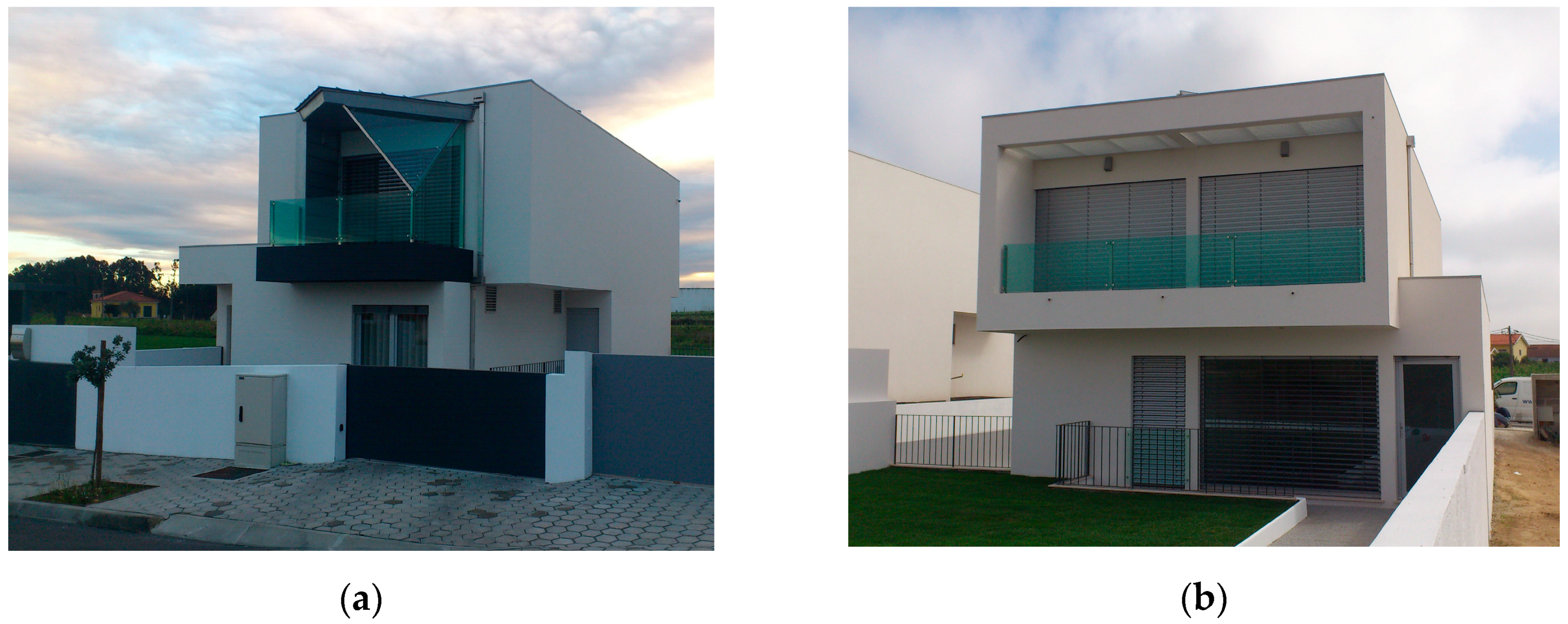
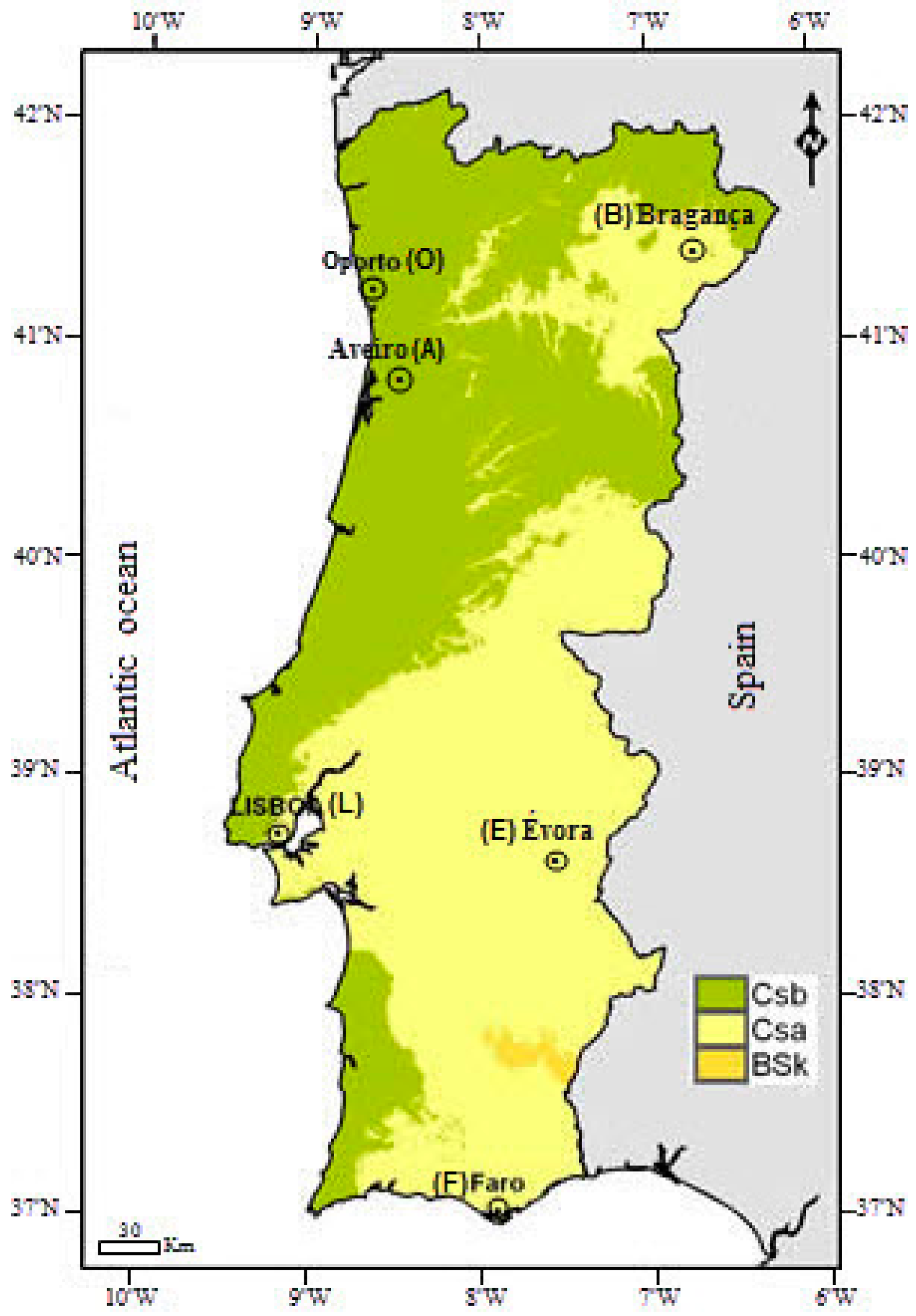
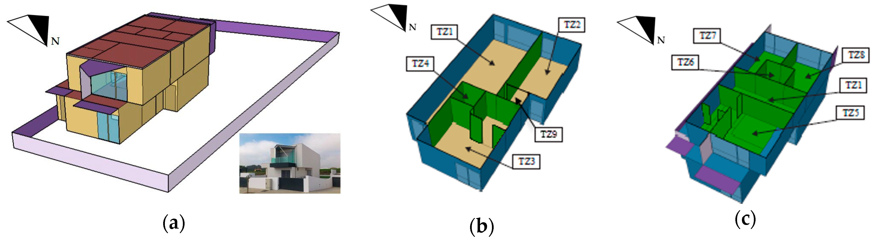
3.1. Building Location and General Characterisation
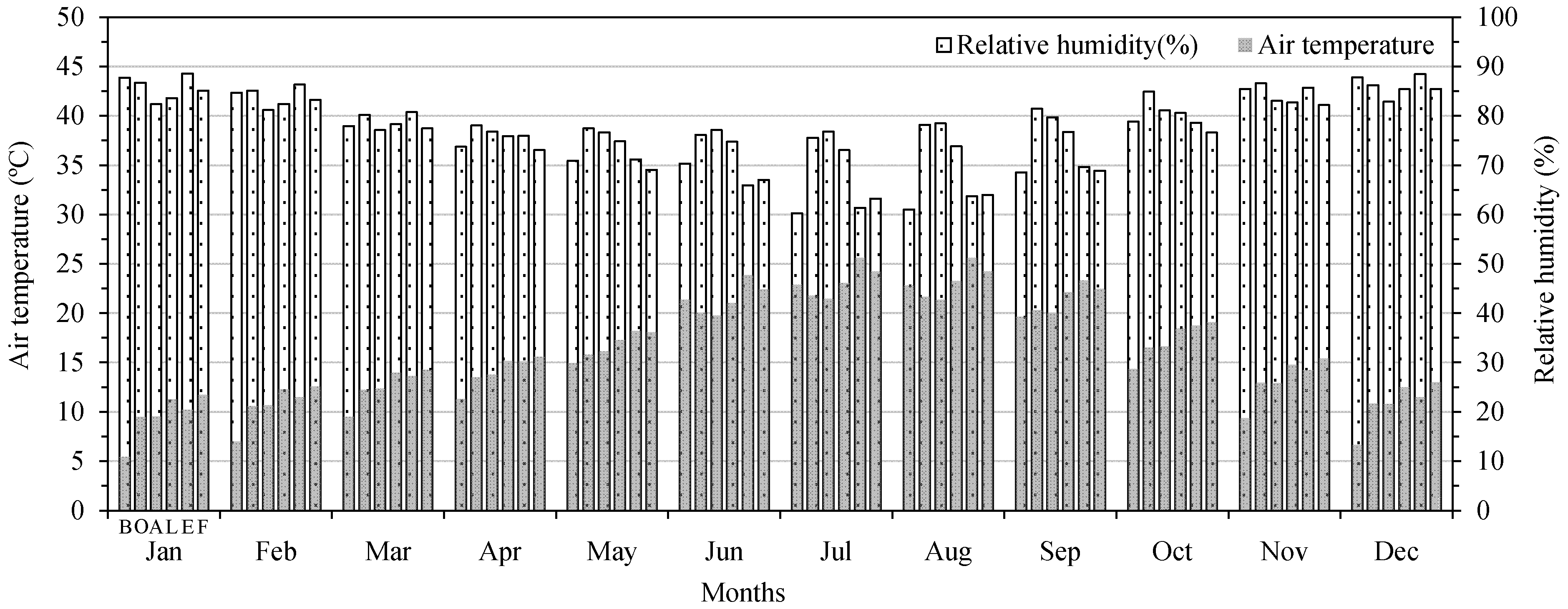
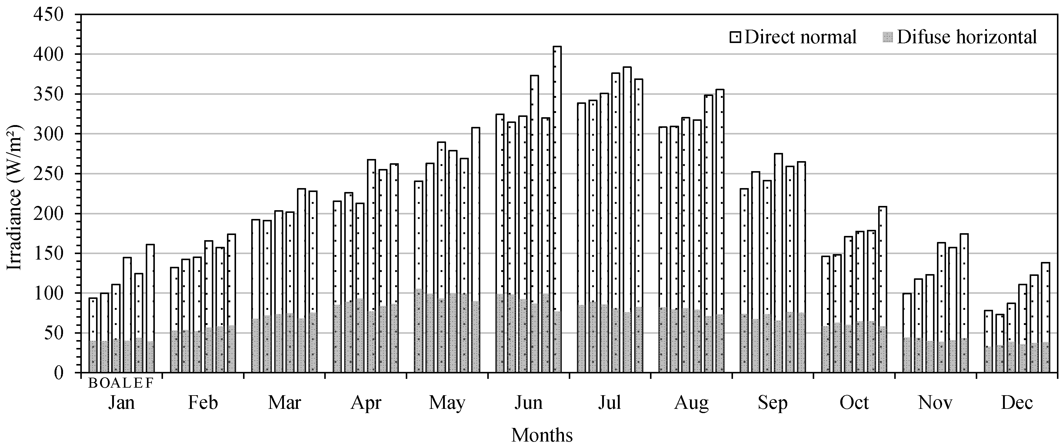
3.2. Weather Files Considered for BEM
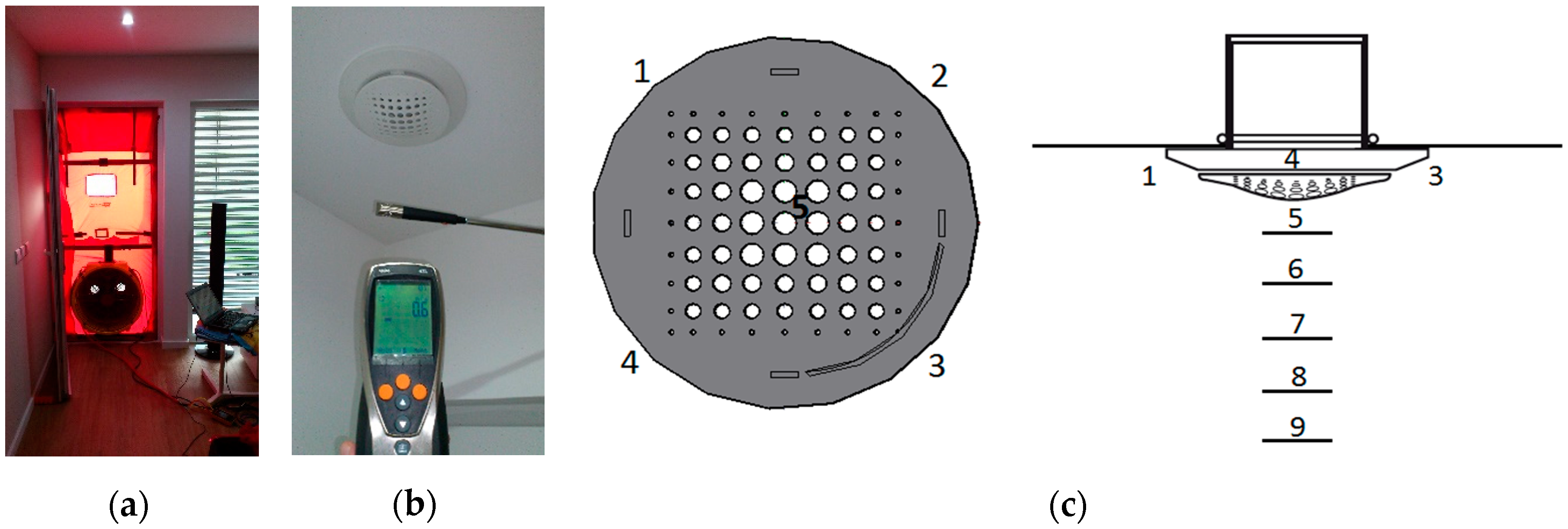
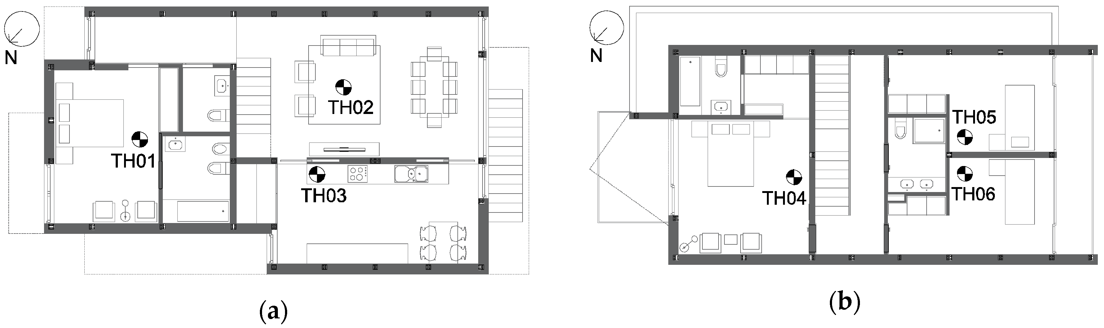
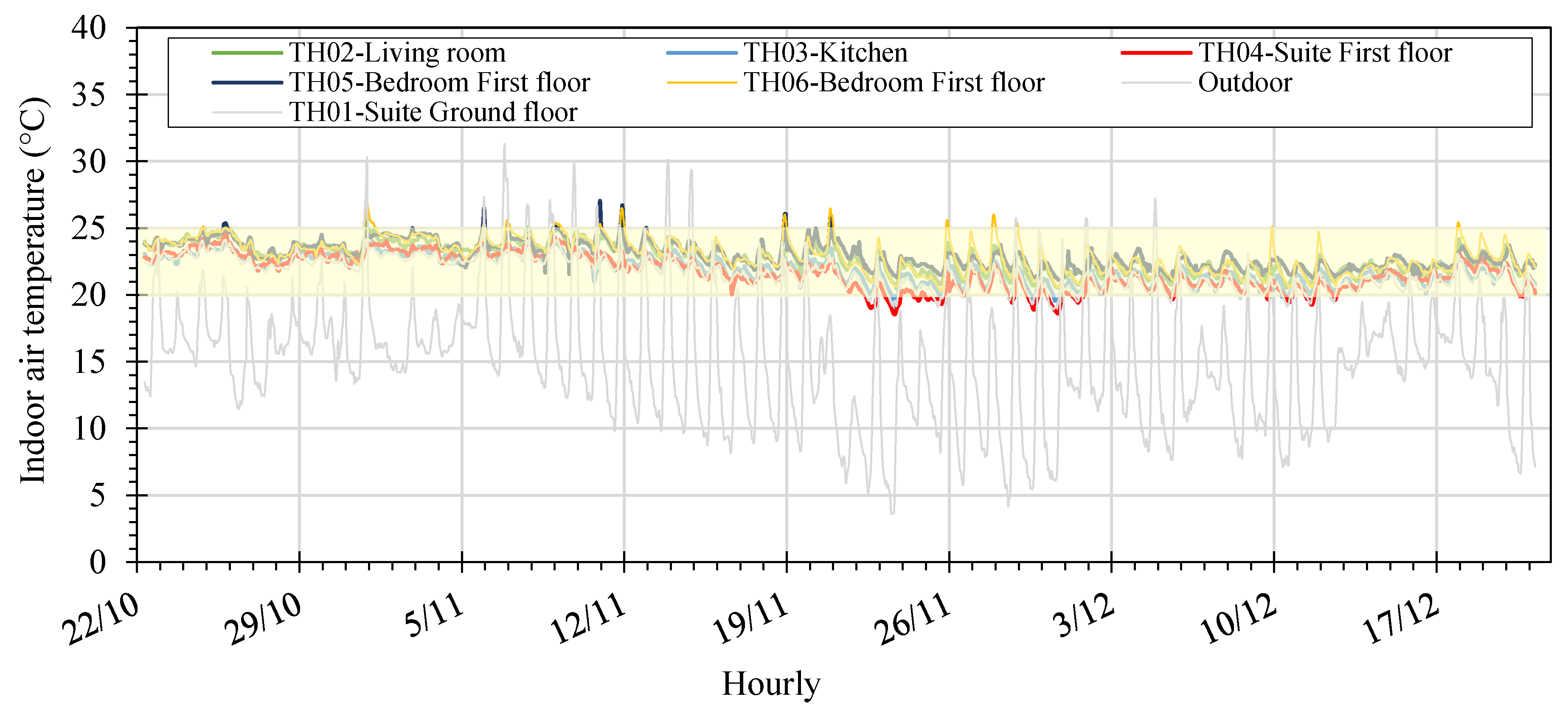
3.3. Monitoring of the Building
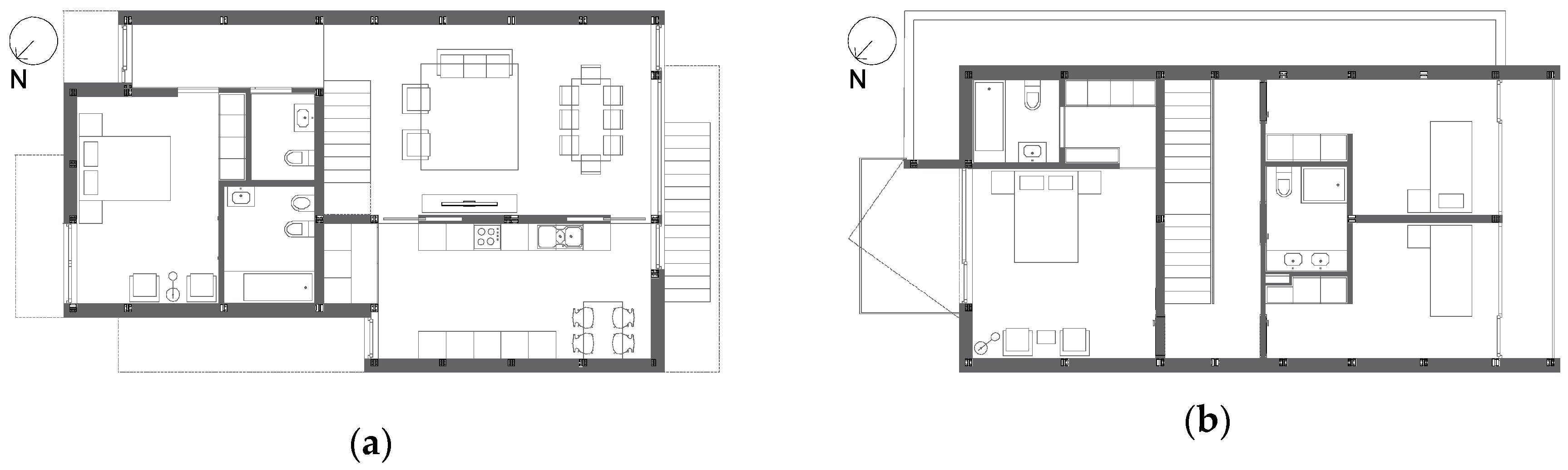
3.4. Numerical Model Definition
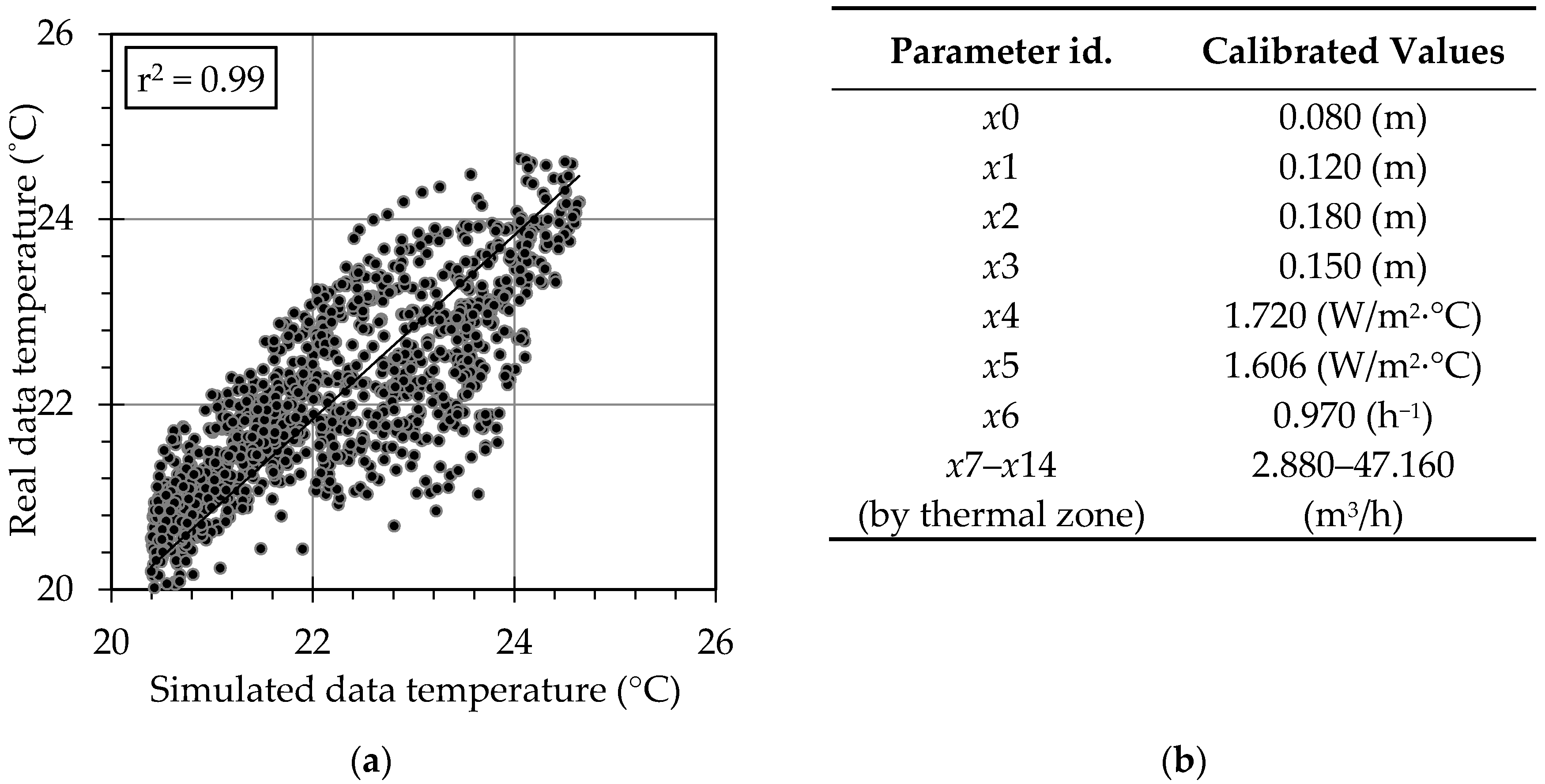
4. Model Calibration
4.1. Definition of the Unknown Parameters
4.2. Accuracy Criteria for the Building Energy Model
4.3. Evaluation of the Calibration Procedure
5. Passive House Optimisation for Different Regions
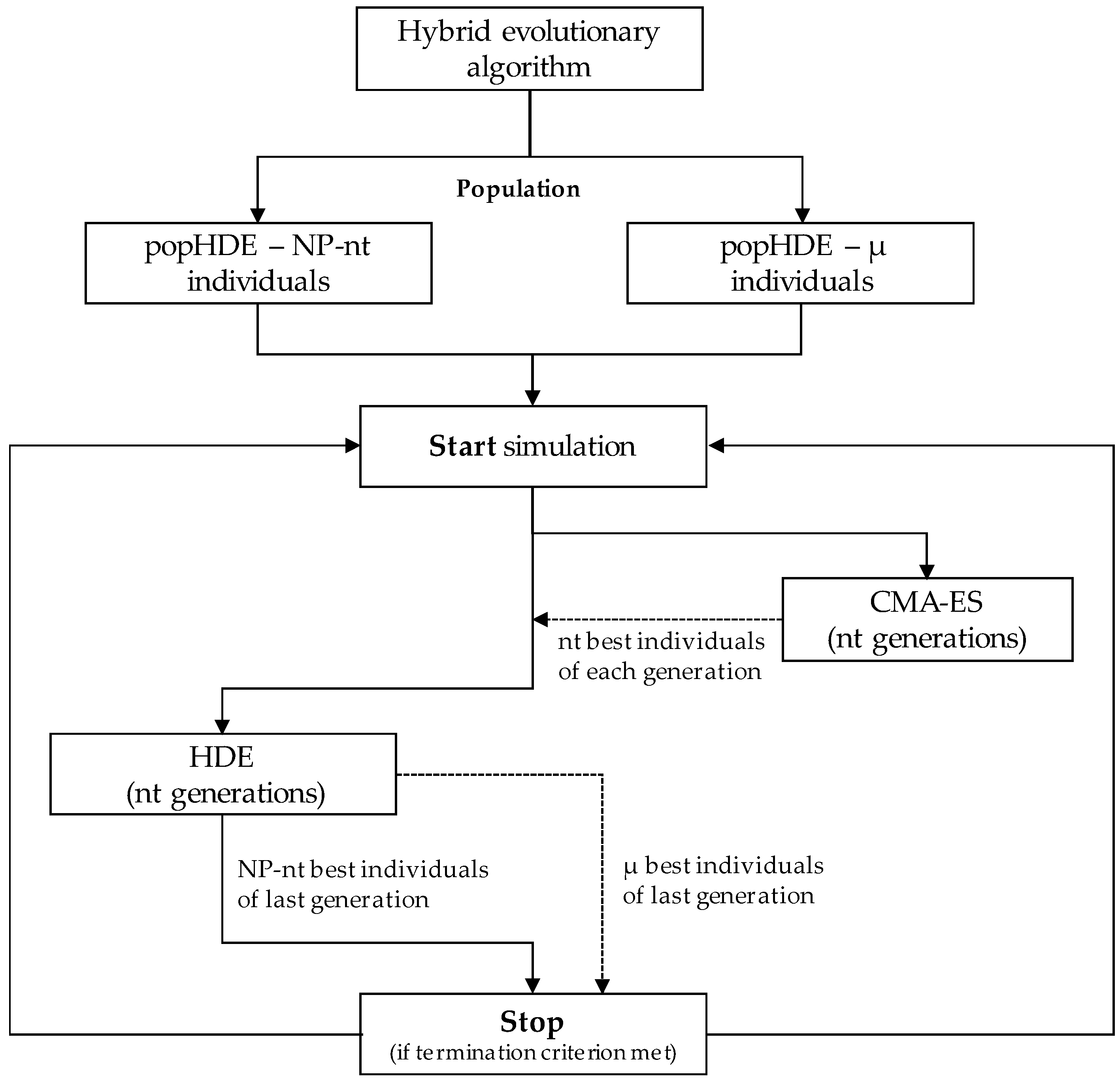
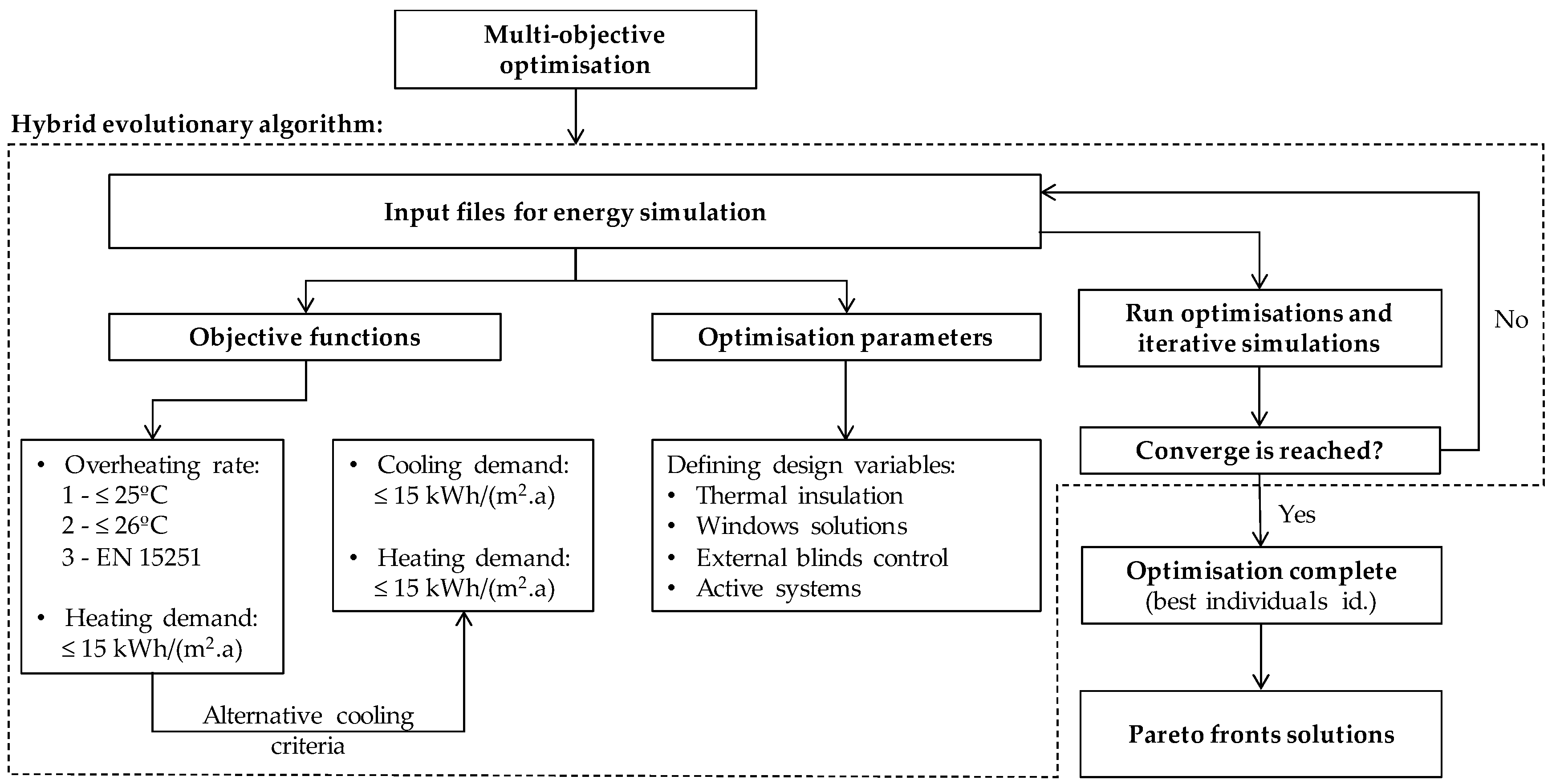
5.1. Multi-Objective Optimisation Using Evolutionary Algorithm
5.2. Objective Functions
5.3. Optimisation Parameters
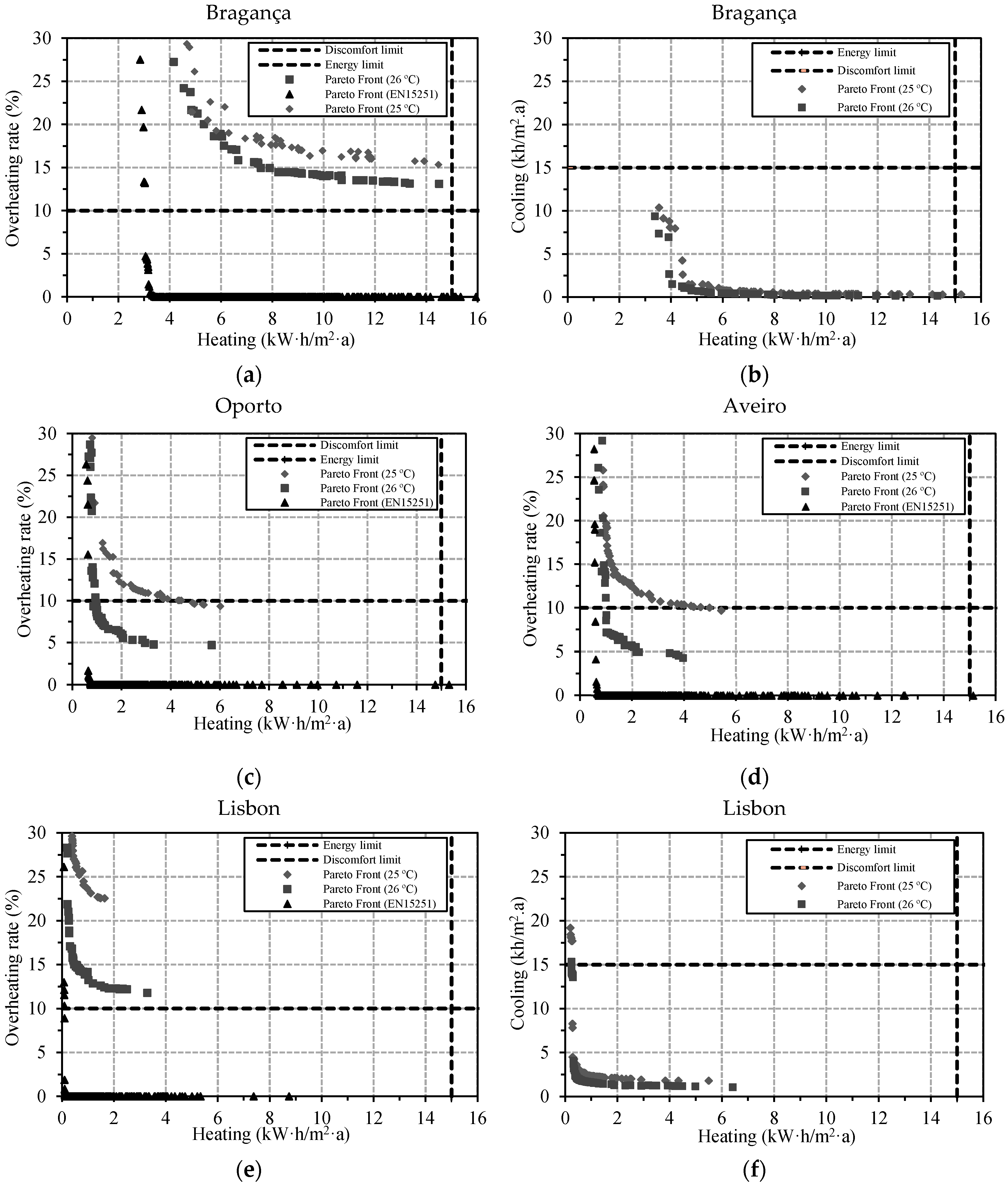
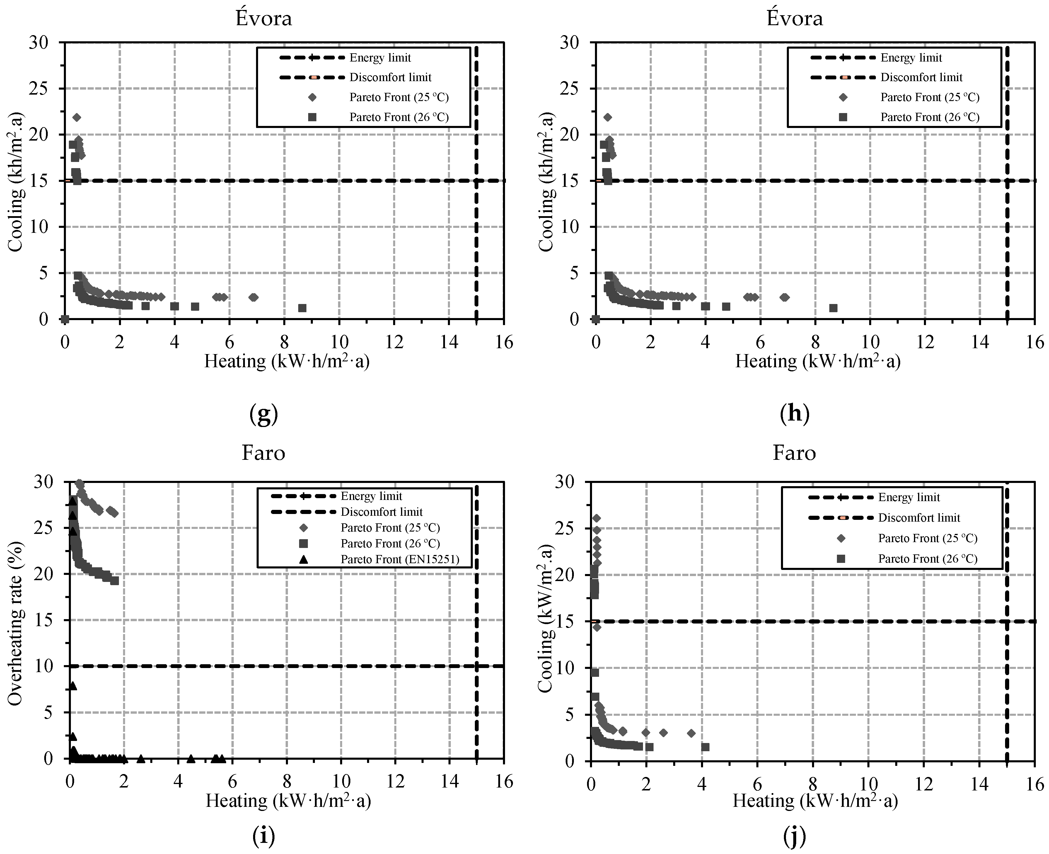
5.4. Numerical Results
5.5. Discussion
6. Life Cycle Costs Analysis
7. Conclusions
Author Contributions
Conflicts of Interest
References
- EPBD. Energy Performance of Buildings Directive 2010/31/EU (recast). In Official Journal of the European Union; European Commision: Brussels, Belgium, 2010; pp. 13–35. [Google Scholar]
- ADENE. Guia Da Eficiência Energética (Guide of Energy Efficiency); ADENE: Lisboa, Portugal, 2012; p. 94. (In Portuguese) [Google Scholar]
- REH. Regulamento de Desempenho Energético de Edifícios de Habitação (Portuguese Regulation on the Energy Performance of Residential Buildings). In Decree-Law No. 118/2013; Diário Da República—1.a Série—N° 159; REH: Lisbon, Portugal, 2013. (In Portuguese) [Google Scholar]
- RECS. Regulamento de Desempenho Energético dos Edifícios de Comércio e Serviços (Service Buildings Regulation). In Decree-Law No. 118/2013; Diário Da República—1.a Série—N° 159; RECS: Lisbon, Portugal, 2013. (In Portuguese) [Google Scholar]
- IPCC. Working Group III: Mitigation of Climate Change, Intergovernmental Panel on Climate; IPCC: Geneva, Switzerland, 2014. [Google Scholar]
- IEE. Very Low-Energy House Concepts in North European Countries; IEE (Intelligent Energy Europe): Brussels, Belgium, 2012. [Google Scholar]
- PHI. Passive House Institute; PHI: Darmstadt, Germany, 2016. [Google Scholar]
- Magnier, L.; Haghighat, F. Multiobjective optimization of building design using TRNSYS simulations, genetic algorithm, and Artificial Neural Network. Build. Environ. 2010, 45, 739–746. [Google Scholar] [CrossRef]
- Kämpf, J.H.; Robinson, D. A simplified thermal model to support analysis of urban resource flows. Energy Build. 2007, 39, 445–453. [Google Scholar] [CrossRef]
- Figueiredo, A.; Kämpf, J.; Vicente, R. Passive house optimization for Portugal: Overheating evaluation and energy performance. Energy Build. 2016, 118, 181–196. [Google Scholar] [CrossRef]
- Crawley, D.B.; Hand, J.W.; Kummert, M.; Griffith, B.T. Contrasting the capabilities of building energy performance simulation programs. Build. Environ. 2008, 43, 661–673. [Google Scholar] [CrossRef] [Green Version]
- Wang, W.; Zmeureanu, R.; Rivard, H. Applying multi-objective genetic algorithms in green building design optimization. Build. Environ. 2005, 40, 1512–1525. [Google Scholar] [CrossRef] [Green Version]
- Tronchin, L.; Fabbri, K. Energy performance building evaluation in Mediterranean countries: Comparison between software simulations and operating rating simulation. Energy Build. 2008, 40, 1176–1187. [Google Scholar] [CrossRef]
- Kämpf, J.H.; Wetter, M.; Robinson, D. A comparison of global optimization algorithms with standard benchmark functions and real-world applications using EnergyPlus. J. Build. Perform. Simul. 2010, 3, 103–120. [Google Scholar] [CrossRef] [Green Version]
- Shorrock, L.; Dunster, J. The physically-based model BREHOMES and its use in deriving scenarios for the energy use and carbon dioxide emissions of the UK housing stock. Energy Policy 1997, 25, 1027–1037. [Google Scholar] [CrossRef]
- Jones, P.J.; Williams, J.; Lannon, S. An energy and environmental prediction tool for planning sustainability in cities. In Proceedings of the 2nd European Conference REBUILD, Florence, Italy, 1–3 April 1998. [Google Scholar]
- Robinson, D.; Campbell, N.; Gaiser, W.; Kabel, K.; Le-Mouel, A.; Morel, N.; Page, J.; Stankovic, S.; Stone, A. SUNtool—A new modelling paradigm for simulating and optimising urban sustainability. Sol. Energy 2007, 81, 1196–1211. [Google Scholar] [CrossRef]
- Robinson, D.; Baker, N. Simplified modelling recent developments in the LT Method. Build. Perform. 2000, 3, 14–19. [Google Scholar]
- Kämpf, J.H.; Robinson, D. A hybrid CMA-ES and HDE optimisation algorithm with application to solar energy potential. Appl. Soft Comput. 2009, 9, 738–745. [Google Scholar] [CrossRef]
- Figueiredo, A.; Figueira, J.; Vicente, R.; Maio, R. Thermal comfort and energy performance: Sensitivity analysis to apply the Passive House concept to the Portuguese climate. Build. Environ. 2016, 103, 276–288. [Google Scholar] [CrossRef]
- Figueiredo, A.; Kämpf, J.; Vicente, R.; Oliveira, R.; Silva, T. Comparison between monitored and simulated data using evolutionary algorithms: Reducing the performance gap in dynamic building simulation. J. Build. Eng. 2018, 17, 96–106. [Google Scholar] [CrossRef]
- Figueiredo, A.; Vicente, R.; Lapa, J.; Cardoso, C.; Rodrigues, F.; Kämpf, J. Indoor thermal comfort assessment using different constructive solutions incorporating PCM. Appl. Energy 2017, 208, 1208–1221. [Google Scholar] [CrossRef]
- Hasan, A.; Vuolle, M.; Siren, K. Minimisation of life cycle cost of a detached house using combined simulation and optimisation. Build. Environ. 2008, 43, 2022–2034. [Google Scholar] [CrossRef]
- Badea, A.; Baracu, T.; Dinca, C.; Tutica, D.; Grigore, R.; Anastasiu, M. A life-cycle cost analysis of the passive house “POLITEHNICA” from Bucharest. Energy Build. 2014, 80, 542–555. [Google Scholar] [CrossRef]
- Ekström, T.; Bernardo, R.; Blomsterberg, Å. Cost-effective passive house renovation packages for Swedish single-family houses from the 1960s and 1970s. Energy Build. 2018, 161, 89–102. [Google Scholar] [CrossRef]
- Tokarik, M.S.; Richman, R.C. Life cycle cost optimization of passive energy efficiency improvements in a Toronto house. Energy Build. 2016, 118, 160–169. [Google Scholar] [CrossRef]
- Almeida, R.M.S.F.; De Freitas, V.P. An insulation thickness optimization methodology for school buildings rehabilitation combining artificial neural networks and life cycle cost. J. Civ. Eng. Manag. 2016, 22, 915–923. [Google Scholar] [CrossRef]
- European Committee for Standardization. EN ISO 10211, Thermal Bridges in Building Construction. Heat Flows and Surface Temperatures—Detailed Calculations; European Committee for Standardization: Brussels, Belgium, 2007; pp. 1–60. [Google Scholar]
- European Committee for Standardization. EN ISO 10077-1, Thermal Performance of Windows, Doors and Shutters—Calculation of Thermal Transmittance—Part 1: General; European Committee for Standardization: Brussels, Belgium, 2006; Volume 1. [Google Scholar]
- Kottek, M.; Grieser, J.; Beck, C.; Rudolf, B.; Rubel, F. World Map of the Köppen-Geiger climate classification updated. Meteorol. Z. 2006, 15, 259–263. [Google Scholar] [CrossRef]
- IPMA, Instituto Português do Mar e da Atmosfera. 2017. Available online: www.ipma.pt (accessed on 1 February 2017).
- Aguiar, R. Clim. e Anos Meteorológicos de Referência para o Sist. Nac. de Certificação de Edifícios (versão 2013), Relatório Para ADENE—Agência de Energia; Lisboa, I.P., Ed.; Laboratório Nacional de Energia e Geologia: Amadora, Portugal, 2013; Volume 55. [Google Scholar]
- International Organization for Standardization. EN ISO 7766, Ergonomics of the Thermal Environment, Instruments for Measuring Physical Quantities; International Organization for Standardization: Geneva, Switzerland, 1998. [Google Scholar]
- Cipriano, J.; Mor, G.; Chemisana, D.; Pérez, D.; Gamboa, G.; Cipriano, X. Evaluation of a multi-stage guided search approach for the calibration of building energy simulation models. Energy Build. 2015, 87, 370–385. [Google Scholar] [CrossRef]
- Passive-On. The Passivhaus Standard in European Warm Climates: Design Guidelines for Comfortable Low Energy Homes; Efficiency Research Group of Polytechnic of Milan: Milan, Italy, 2006. [Google Scholar]
- Vidal, F.; Meireles, I.; Vicente, R.; Sousa, V.; Rodrigues, F. Thermal comfort performance of a passive house in summer under a Mediterranean climatein. In Proceedings of the 41st IAHS World Congress—Sustainability Innovation for the Future, Albufeira, Portugal, 13–16 September 2016. [Google Scholar]
- ASHRAE. ASHRAE Guideline 14-2002 Measurement of Energy and Demand Savings, American Society of Heating. Refrig. Air-Cond. Eng. 2002, 8400, 170. [Google Scholar]
- IPMVP. International Performance Measurement and Verification Protocol, Concepts and Options for Determining Energy and Water Savings; International Performance Measurement and Verification Protocol Committee: Washington, DC, USA, 2002; Volume 1. [Google Scholar]
- FEMP, US DOE. M&V Guidelines: Measurement and Verification for Federal Energy Projects Version 3.0, Federal Energy Management Program; US Department of Energy: Washington, DC, USA, 2008.
- Bou-Saada, T.E.; Haberl, J.S. An Improved Procedure for Developing Calibrated Hourly Simulation Models; IBPSA-USA: Washington, MI, USA, 1995. [Google Scholar]
- Kreider, J.F.; Haberl, J.S. Predicting hourly building energy usage. ASHRAE J. 1994, 36, 6. [Google Scholar]
- Kreider, J.F.; Haberl, J.S. Predicting hourly building energy use: The great energy predictor shootout: Overview and discussion of results. ASHRAE Trans. Res. 1994, 100, 1104–1118. [Google Scholar]
- European Committee for Standardization. EN 15251, Indoor Environmental Input Parameters for Design and Assessment of Energy Performance of Buildings Addressing Indoor Air Quality, Thermal Environment, Lighting and Acoustics; European Committee for Standardization: Brussels, Belgium, 2007. [Google Scholar]
- Wu, Z.; Xia, X.; Wang, B. Improving building energy efficiency by multiobjective neighborhood field optimization. Energy Build. 2015, 87, 45–56. [Google Scholar] [CrossRef]
- Schnieders, J.; Feist, W.; Rongen, L. Passive Houses for different climate zones. Energy Build. 2015, 105, 71–87. [Google Scholar] [CrossRef]
- Feist, W.; Schnieders, J.; Dorer, V.; Haas, A. Re-inventing air heating: Convenient and comfortable within the frame of the Passive House concept. Energy Build. 2005, 37, 1186–1203. [Google Scholar] [CrossRef]
- Fuller, S.K.; Petersen, S.R. NIST Handbook 135: Life-Cycle Costing Manual for the Federal Energy Management Program; National Institute of Standards and Technology: Gaithersburg, MD, USA, 1996; Volume 5. [Google Scholar]
- Santos, P.; Gervásio, H.; da Silva, L.S.; Lopes, A.G. Influence of climate change on the energy efficiency of light-weight steel residential buildings. Civ. Eng. Environ. Syst. 2011, 28, 325–352. [Google Scholar] [CrossRef]


| Ground Floor Slab | External Walls | Flat Roof |
|---|---|---|
 | 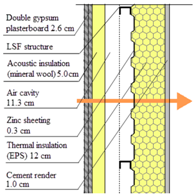 | 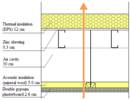 |
| Uvalue = 0.32 W/(m2·°C) | Uvalue = 0.21 W/(m2·°C) | Uvalue = 0.21 W/(m2·°C) |
| Thermal Zone | Level * (%) | Profile | |||
|---|---|---|---|---|---|
| Week Day | Weekend | ||||
| TZ01 | 25 50 100 25 | On From | 15:00 to 16:00 18:00 to 20:00 20:00 to 22:00 22.00 to 23.00 | On From | - 22:00 to:24.00 14:00 to 21:00 - |
| TZ02 | 25 50 50 | 7:00 to 8:00 15:00 to 16:00 19:00 to 20:00 | 7:00 to 8:00 15:00 to 16:00 19:00 to 20:00 | ||
| TZ03/TZ05/TZ07/TZ08 | 100 100 | 00:00 to 8:00 21:00 to 24:00 | 00:00 to 8:00 21:00 to 24:00 | ||
| Parameter id. | Designation (Units) | Box Constraints Limits |
|---|---|---|
| x0 | Ground floor insulation thickness (m) | 0.080–0.100 |
| x1 | External wall insulation thickness (m) | 0.114–0.120 |
| x2 | Roof insulation thickness—Ground floor level (m) | 0.160–0.180 |
| x3 | Roof insulation thickness—First floor level (m) | 0.130–0.150 |
| x4 | North windows: Uvalue (W/m2·°C) | 1.634–1.806 |
| x5 | South windows: Uvalue (W/m2·°C) | 1.606–1.775 |
| x6 | Infiltration rate at 50 Pa (h−1) | 0.300–1.500 |
| x7–x14 (by thermal zone) | Air change rate (m3/h) | 2.700–70.540 |
| Calibration Results—id# 10298 | Hourly Criteria (%) | ||||
|---|---|---|---|---|---|
| NMBE | RMSE | CV RMSE | GOF | Standards | CV RMSE Limits |
| −0.65 | 0.72 | 3.28 | 2.36 | ASHRAE Guideline | 30 |
| IPMVP | 20 | ||||
| FEMP | 30 | ||||
| Parameter id. | Designation | Box Constraints |
|---|---|---|
| #00 | Pavement insulation thickness (m) | 0.060–0.240 |
| #01 | Wall insulation thickness (m) | 0.020–0.240 |
| #02 | Roof insulation thickness (m) | 0.040–0.300 |
| #03 | Exterior windows North (-) | Defined as discrete variables (Table 6) |
| #04 | Exterior windows South (-) | |
| #05 | Blinds: slat angle (°) | 5.000–90.00 |
| #06 | Blinds: activation by temperature (°C) | ≥21.00 |
| #07 | Bypass: air flow rate (h−1) | 0.000–1.800 |
| #08 | Bypass: activation temperature (°C) | 21.00–26.00 |
| #09 to #16 (by thermal zone) | Air change rate (h−1) | 0.300–0.600 |
| #17 | Activate system solution | Defined as discrete variable |
| Solution (Si) | S1 | S2 | S3 | S4 | S5 | S6 |
|---|---|---|---|---|---|---|
| Glazing Type | Double Glazing | Triple Glazing | ||||
| Uf Ug SHGC | 1.50 | 1.50 | 1.50 | 1.50 | 1.50 | 1.10 |
| 1.40 | 1.40 | 1.50 | 1.40 | 1.40 | 0.60 | |
| 0.38 | 0.48 | 0.57 | 0.62 | 0.71 | 0.54 | |
| INPUTS | |||||||||||||||||||
|---|---|---|---|---|---|---|---|---|---|---|---|---|---|---|---|---|---|---|---|
| Case | Parameters | #00 | #01 | #02 | #03 * | #04 * | #05 | #06 | #07 | #08 | #09 | #10 | #11 | #12 | #13 | #14 | #15 | #16 | #17 * |
| Bragança | m ± s | 0.115 ± 0.070 | 0.234 ± 0.015 | 0.296 ± 0.010 | S6 | S6 | 8.705 ± 14.477 | 22.540 ± 3.135 | 22.385 ± 1.547 | 0.556 ± 0.547 | 52.921 ± 13.890 | 31.350 ± 2.107 | 31.545 ± 8.509 | 4.062 ± 0.977 | 24.776 ± 6.240 | 6.654 ± 1.902 | 14.295 ± 3.947 | 17.421 ± 4.345 | MVHR |
| CV (%) | 60.7 | 6.6 | 3.5 | 166.3 | 13.9 | 6.9 | 98.5 | 26.2 | 6.7 | 27.0 | 24.1 | 25.2 | 28.6 | 27.6 | 24.9 | ||||
| Oporto | m ± s | 0.194 ± 0.049 | 0.238 ± 0.007 | 0.298 ± 0.008 | S6 | S6 | 5.019 ± 0.083 | 22.389 ± 0.846 | 21.190 ± 0.478 | 1.752 ± 0.088 | 37.357 ± 3.322 | 24.538 ± 3.837 | 23.063 ± 2.249 | 3.793 ± 0.690 | 23.670 ± 4.149 | 5.799 ± 0.845 | 13.658 ± 2.171 | 13.901 ± 2.417 | MVHR |
| CV (%) | 25.1 | 2.8 | 2.6 | 1.7 | 3.8 | 2.3 | 5.0 | 8.9 | 15.6 | 9.8 | 18.2 | 17.5 | 14.6 | 15.9 | 17.4 | ||||
| Aveiro | m ± s | 0.196 ± 0.051 | 0.239 ± 0.003 | 0.299 ± 0.003 | S6 | S6 | 5.010 ± 0.084 | 22.484 ± 0.895 | 21.279 ± 0.440 | 1.675 ± 0.151 | 47.944 ± 9.460 | 17.013 ± 1.671 | 26.420 ± 5.721 | 3.619 ± 0.583 | 23.336 ± 3.532 | 5.839 ± 1.182 | 20.320 ± 3.318 | 13.218 ± 1.992 | MVHR |
| CV (%) | 25.9 | 1.1 | 0.9 | 1.7 | 4.0 | 2.1 | 9.0 | 19.7 | 9.8 | 21.7 | 16.1 | 15.1 | 20.2 | 16.3 | 15.1 | ||||
| Lisbon | m ± s | 0.166 ± 0.031 | 0.212 ± 0.058 | 0.286 ± 0.022 | S6 | S6 | 7.692 ± 7.617 | 23.544 ± 1.977 | 22.044 ± 0.992 | 1.288 ± 0.272 | 54.447 ± 5.644 | 31.467 ± 1.749 | 36.276 ± 2.842 | 3.683 ± 0.249 | 25.836 ± 3.850 | 9.214 ± 0.805 | 19.218 ± 1.131 | 16.258 ± 1.414 | MVHR |
| CV (%) | 18.9 | 27.4 | 7.6 | 99.0 | 8.4 | 4.5 | 21.1 | 10.4 | 5.6 | 7.8 | 6.8 | 14.9 | 8.7 | 5.9 | 8.7 | ||||
| Évora | m ± s | 0.142 ± 0.055 | 0.221 ± 0.040 | 0.285 ± 0.024 | S6 | S6 | 5.608 ± 3.210 | 22.875 ± 1.414 | 21.813 ± 1.218 | 1.046 ± 0.622 | 44.490 ± 10.257 | 31.662 ± 1.063 | 31.869 ± 8.380 | 4.107 ± 0.902 | 33.669 ± 7.310 | 6.940 ± 1.782 | 16.501 ± 3.728 | 19.777 ± 3.232 | MVHR |
| CV (%) | 38.9 | 18.3 | 8.3 | 57.2 | 6.2 | 5.6 | 59.5 | 23.1 | 3.4 | 26.3 | 22.0 | 21.7 | 25.7 | 22.6 | 16.3 | ||||
| Faro | m ± s | 0.085 ± 0.038 | 0.224 ± 0.045 | 0.294 ± 0.013 | S6 | S6 | 7.100 ± 11.183 | 22.485 ± 1.421 | 22.191 ± 1.438 | 1.587 ± 0.327 | 52.307 ± 11.044 | 31.558 ± 0.935 | 30.419 ± 5.950 | 4.056 ± 0.624 | 26.478 ± 5.447 | 9.455 ± 1.030 | 14.252 ± 2.436 | 13.587 ± 2.462 | MVHR |
| CV (%) | 44.9 | 20.3 | 4.5 | 157.5 | 6.3 | 6.5 | 20.6 | 21.1 | 3.0 | 19.6 | 15.4 | 20.6 | 10.9 | 17.1 | 18.1 | ||||
| Thermal Insulation | Windows | ||||
|---|---|---|---|---|---|
| Thickness (m) | Costs | Solutions | Costs | ||
| Material/Application (€/m2) | Maintenance (€/year) | Material/Application (€/m2) | Maintenance (€/year) | ||
| 0.00 to 0.03 | 5.09 | 7.01 | S1 | 1815.26 | 27.22 |
| 0.04 to 0.07 | 9.34 | 7.67 | S2 | 1760.69 | 28.19 |
| 0.08 to 0.11 | 15.28 | 8.67 | S3 | 1721.07 | 26.07 |
| 0.12 to 0.15 | 23.20 | 10.30 | S4 | 1699.89 | 23.38 |
| 0.16 to 0.19 | 28.86 | 11.65 | S5 | 1674.23 | 24.48 |
| 0.20 to 0.23 | 35.65 | 12.85 | |||
| 0.24 to 0.27 | 42.43 | 14.43 | S6 | 2280.73 | 30.87 |
| 0.28 to 0.30 | 49.23 | 15.79 | |||
| City | Bragança | Oporto | Aveiro | Lisbon | Évora | Faro |
|---|---|---|---|---|---|---|
| Id./Variable | 118 | 229 | 18 | 328 | 376 | 465 |
| #00 | 0.061 | 0.096 | 0.146 | 0.126 | 0.080 | 0.060 |
| #01 | 0.147 | 0.233 | 0.239 | 0.023 | 0.020 | 0.030 |
| #02 | 0.263 | 0.277 | 0.300 | 0.280 | 0.300 | 0.270 |
| #03 * | S6 | S6 | S6 | S1 | S2 | S3 |
| #04 * | S4 | S5 | S6 | S1 | S4 | S6 |
| #05 | 5.000 | 5.000 | 5.000 | 5.713 | 5.000 | 5.000 |
| #06 | 21.000 | 22.576 | 22.070 | 22.401 | 21.000 | 21.000 |
| #07 | 22.762 | 21.059 | 21.000 | 21.973 | 26.000 | 22.049 |
| #08 | 1.241 | 1.749 | 1.649 | 1.280 | 1.800 | 1.800 |
| #09 | 70.280 | 40.578 | 58.190 | 53.504 | 35.280 | 59.204 |
| #10 | 32.040 | 29.975 | 15.840 | 29.942 | 32.040 | 31.409 |
| #11 | 27.961 | 27.250 | 26.150 | 31.340 | 21.960 | 32.900 |
| #12 | 5.400 | 3.131 | 2.911 | 3.607 | 2.880 | 4.613 |
| #13 | 30.315 | 28.448 | 25.699 | 24.212 | 41.760 | 26.519 |
| #14 | 7.011 | 5.050 | 5.084 | 8.822 | 5.040 | 10.080 |
| #15 | 11.583 | 14.145 | 23.040 | 21.235 | 23.040 | 15.154 |
| #16 | 13.994 | 14.633 | 11.520 | 16.219 | 23.040 | 11.520 |
| #17 * | MVHR | MVHR | MVHR | MVHR | MVHR | MVHR |
| LCC (€) | 73,275 | 78,857 | 84,407 | 63,289 | 63,783 | 58,862 |
© 2018 by the authors. Licensee MDPI, Basel, Switzerland. This article is an open access article distributed under the terms and conditions of the Creative Commons Attribution (CC BY) license (http://creativecommons.org/licenses/by/4.0/).
Share and Cite
Oliveira, R.; Figueiredo, A.; Vicente, R.; Almeida, R.M.S.F. Multi-Objective Optimisation of the Energy Performance of Lightweight Constructions Combining Evolutionary Algorithms and Life Cycle Cost. Energies 2018, 11, 1863. https://doi.org/10.3390/en11071863
Oliveira R, Figueiredo A, Vicente R, Almeida RMSF. Multi-Objective Optimisation of the Energy Performance of Lightweight Constructions Combining Evolutionary Algorithms and Life Cycle Cost. Energies. 2018; 11(7):1863. https://doi.org/10.3390/en11071863
Chicago/Turabian StyleOliveira, Rui, António Figueiredo, Romeu Vicente, and Ricardo M. S. F. Almeida. 2018. "Multi-Objective Optimisation of the Energy Performance of Lightweight Constructions Combining Evolutionary Algorithms and Life Cycle Cost" Energies 11, no. 7: 1863. https://doi.org/10.3390/en11071863