Numerical Investigations of the Effects of the Rotating Shaft and Optimization of Urban Vertical Axis Wind Turbines

Abstract
:
1. Introduction
- Analyze the reasons for power coefficient of wind turbines decrease as the ratio of the shaft diameter to the wind turbine diameter (α) increase from 0% to 9% quantitatively.
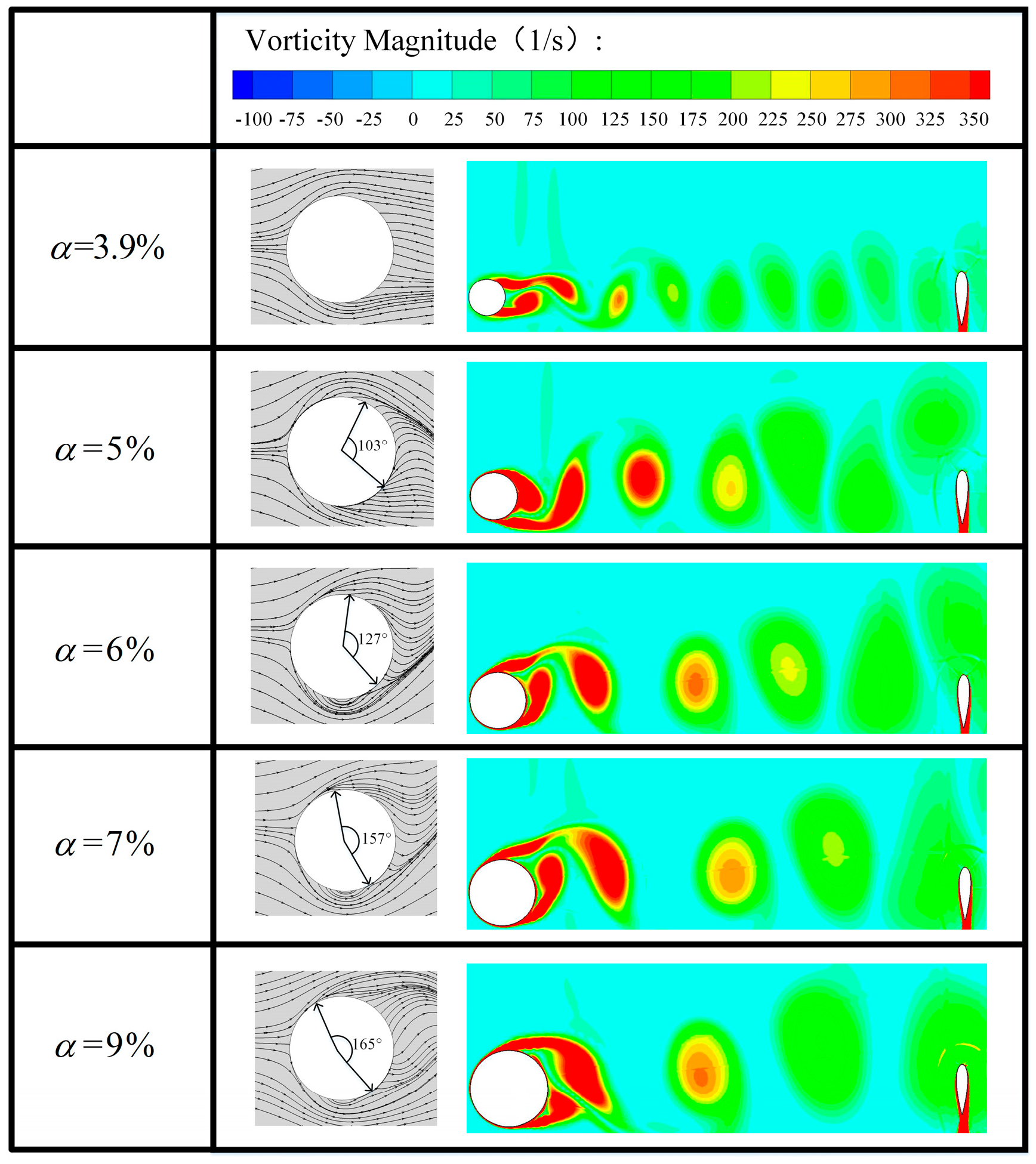
- Investigate the vortex variations behind the rotating shaft of the VAWT and the variations of the boundary separation point as α increase from 0% to 9%.
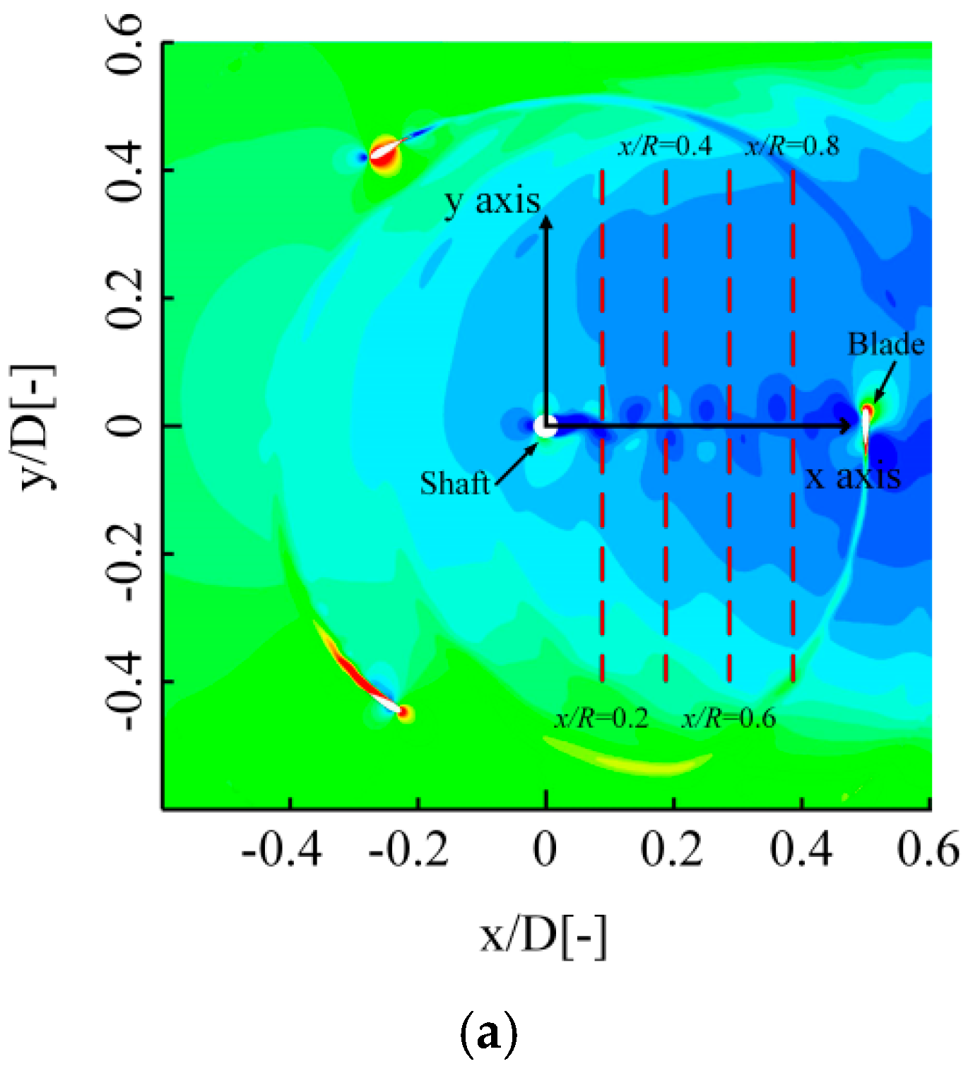
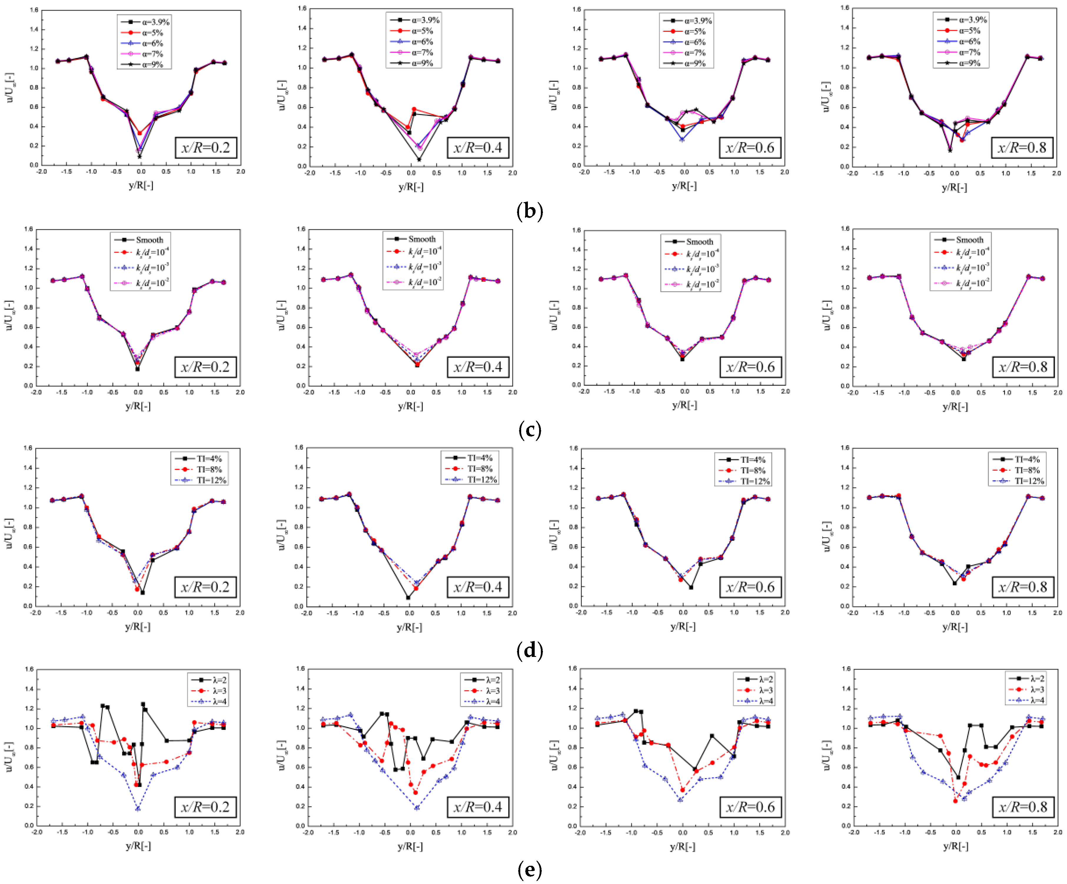
- Explore the wind velocity distribution ruler of the flow field when the vertical axis wind turbine operates under different operating conditions (including TI and TSRs) and physical parameters (including α and ks/ds).
- Many factors can have impacts on the wake effect of the rotating central shaft on the performance of urban VAWTs, for instance, α, TSRs, ks/ds, and TI. One of the purposes of this research is to figure out the influence strength order of these factors, and to find out an optimal operational condition for the VAWT.
2. Numerical Model
2.1. Model Geometry
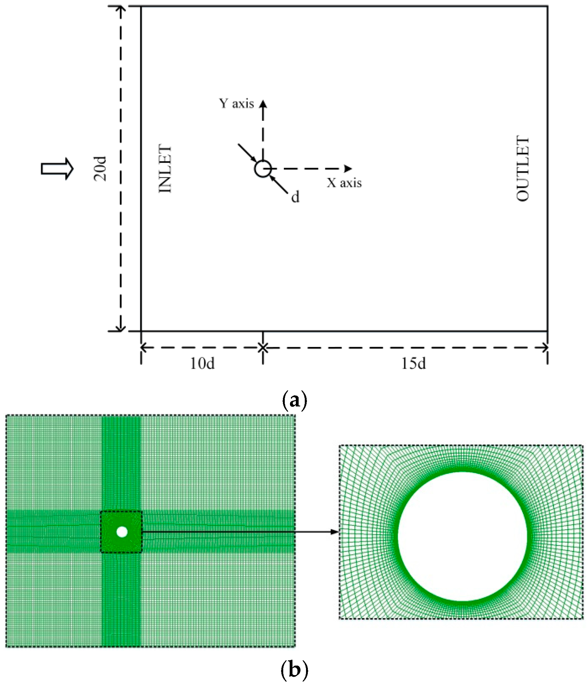
2.2. Computational Domain and Mesh Generation
2.3. Boundary Conditions and Numerical Settings
2.4. Validation Study of Central Cylinder
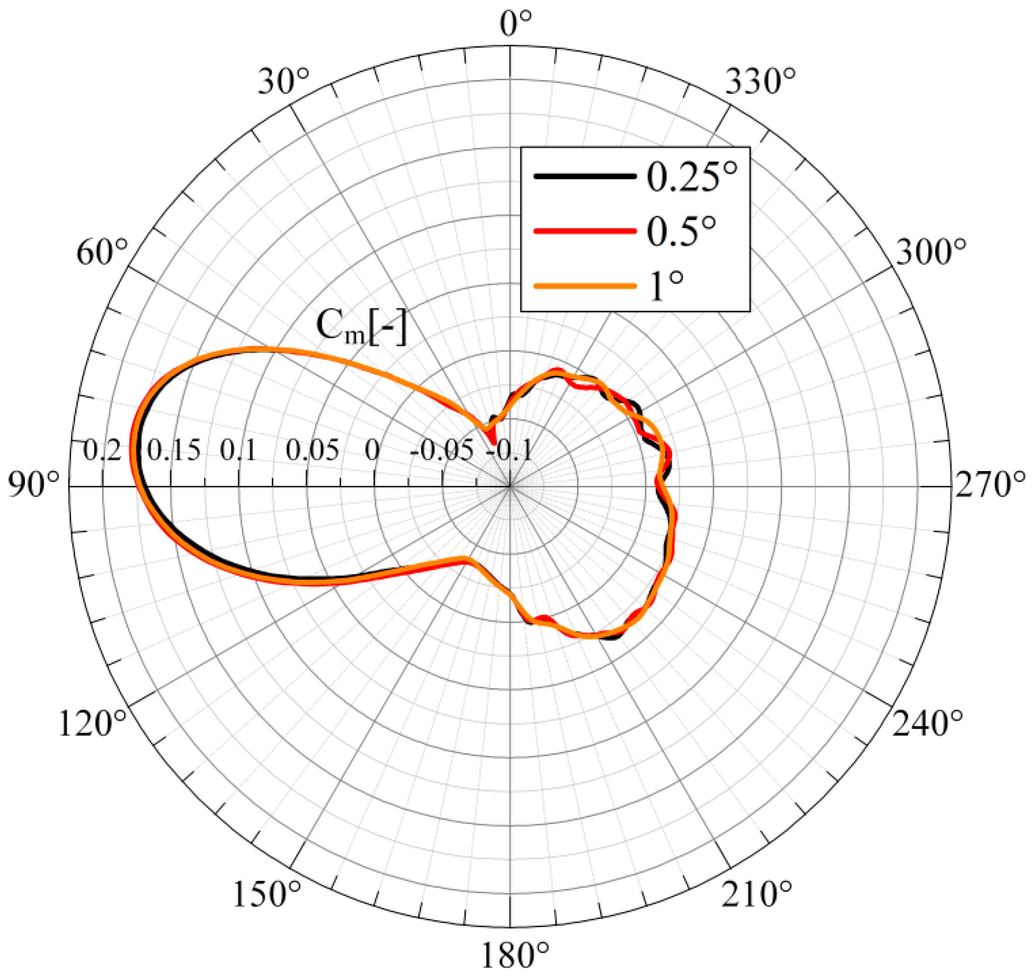
2.5. Grid Independence and Numerical Validation
- (1)
- In the process of measuring the experimental data, a method of spin down tests is used, it leads the actual wind speed acted on the wind turbine is lower than the set wind speed as the presence of blockage effects. Therefore, the measured results will still be small, although some corrections are made during the subsequent data processing.
- (2)
- Since a simplified 2D geometrical model is employed in the simulation and the influence of the blade span and junctions connected the blades and the shaft also not considered in the process of simulating, a deviation might be existed between the experimental results and the simulation results. It is noteworthy that for high TSRs (4 < TSRs < 5), there is a mass of drag can be produced by the junctions connected the blades and the shaft in the actual operation of the VAWT. In addition, the shedding vortices that are generated by the internal junctions during the operation of the VAWT have not been accurately simulated with a 2D simplified model. These reasons have great influence on the prediction results of numerical simulation under high TSRs.
- (3)
- In the course of numerical calculation, the accuracy of using simplified 2D unsteady Reynolds-average Navier-Stokes (URANS) to solve the 3D problem with complex flow characteristics is limited [40]. Especially for the study of blade-wake interactions in this paper. This is also one of the possible reasons for the differences between the simulated predicted results and experimental measurements.
2.6. Taguchi Method
- (a)
- The quality characteristics and control factors need explicit.
- (b)
- Identify the number of levels for the control factors and the interactions between the factors.
- (c)
- List the table of orthogonal array according to the numbers of factors and the levels of each factor.
- (d)
- Implement the experiments based on the arrangement of orthogonal array.
- (e)
- Analyze the experimental results with the signal-to-noise ratio.
- (f)
- Obtain the effect strength order of each influent factor.
- (g)
- Select the optimal levels of each control factor.
3. Results and Discussion
3.1. Influence of Ratio of the Shaft Diameter to the Wind Turbine Diameter on Wind Turbine Performance
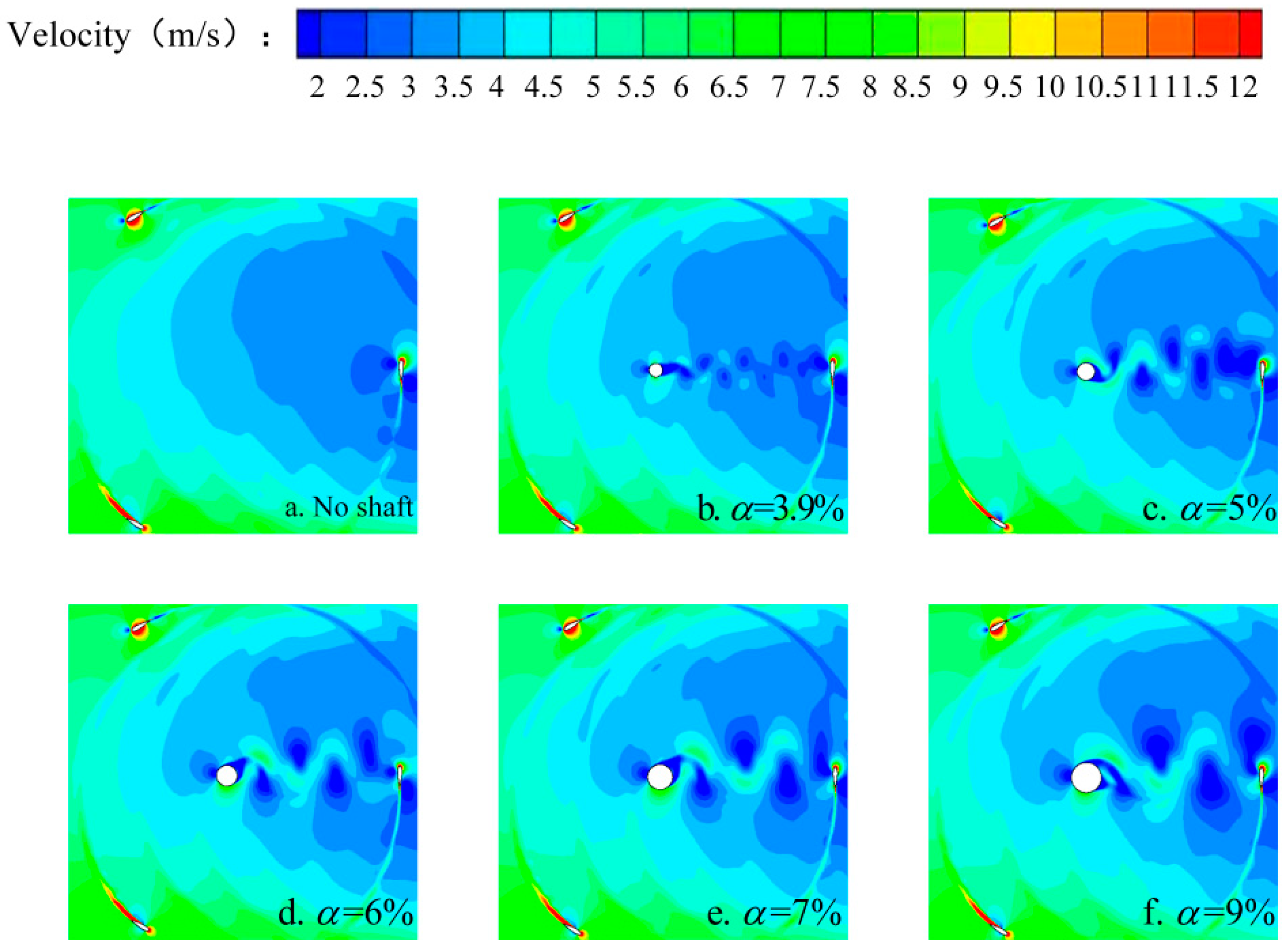
3.2. Analysis of the Flow Characteristics around the Rotating Shaft
3.3. The Influence of Rotating Central Shaft on the Flow Field inside the Wind Turbine
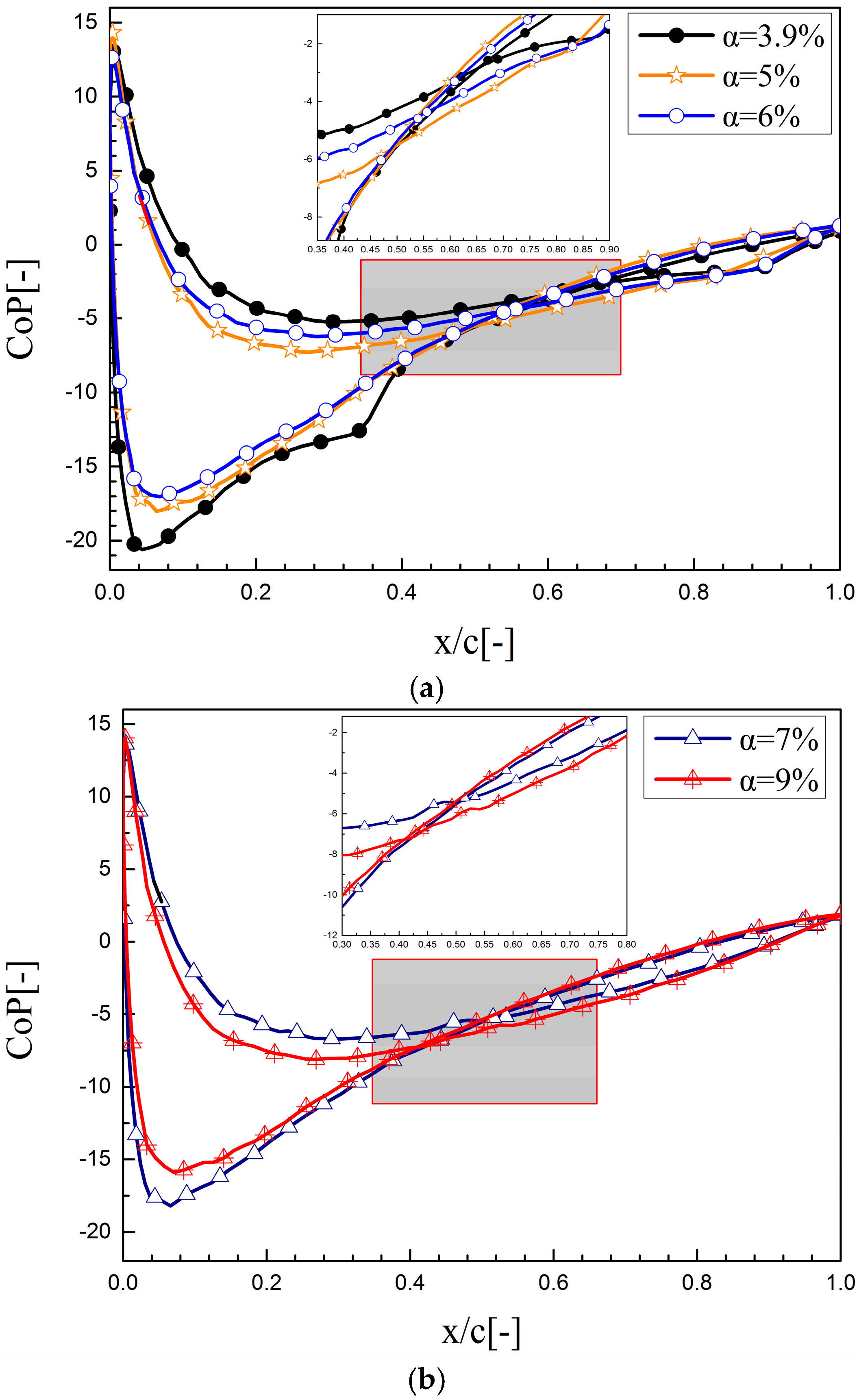
3.4. Influence of Central Rotating Shaft on Flow Field near Blade
4. Performance Analysis of the VAWT with Taguchi Method
4.1. Power Coefficients of VAWT in Taguchi Approach
4.2. Optimum Operation
5. Conclusions
- A minimum instantaneous power coefficient value appears when the wind turbine blade operates at the vicinity of an azimuthal angle of 270°, which indicates that the occurrence of the wake effect that is generated by the central rotating shaft. As α increases to 9%, the wind turbine has a minimum power coefficient value, and the power loss of the wind turbine in one revolution increased from 0% to 25%, relative to that of the no-shaft wind turbine.
- The influence of the wake effect on the downstream velocity field is very strong during the VAWT operation of VAWT. The effect of the shedding vortex, which is exerted by the wind turbine’s rotating shaft, becomes stronger and decreases the pressure gradient between the suction side and pressure side. In addition, the lift that is produced by the blades can be also reduced, and this results in the reduction of the Cp of the wind turbine in one revolution.
- As the value of α increase, the phenomenon of boundary layer separation will become increasingly evident. For the wind turbine model in the present study, α = 5% is a critical point, the shedding vortex released by the rotating shaft alternates periodically when α < 5%. The phenomenon is that the distance between the two vortices at the front and back is small. Subsequently, the front shedding vortex exerts a small effect on the back vortex, and the intensity of the vortices is weak. The shedding vortices released by the central rotating shaft are mostly a single main vortex when α > 5%. The distance between the two vortices in the front and back is large, while the influence exertion on each other is weak.
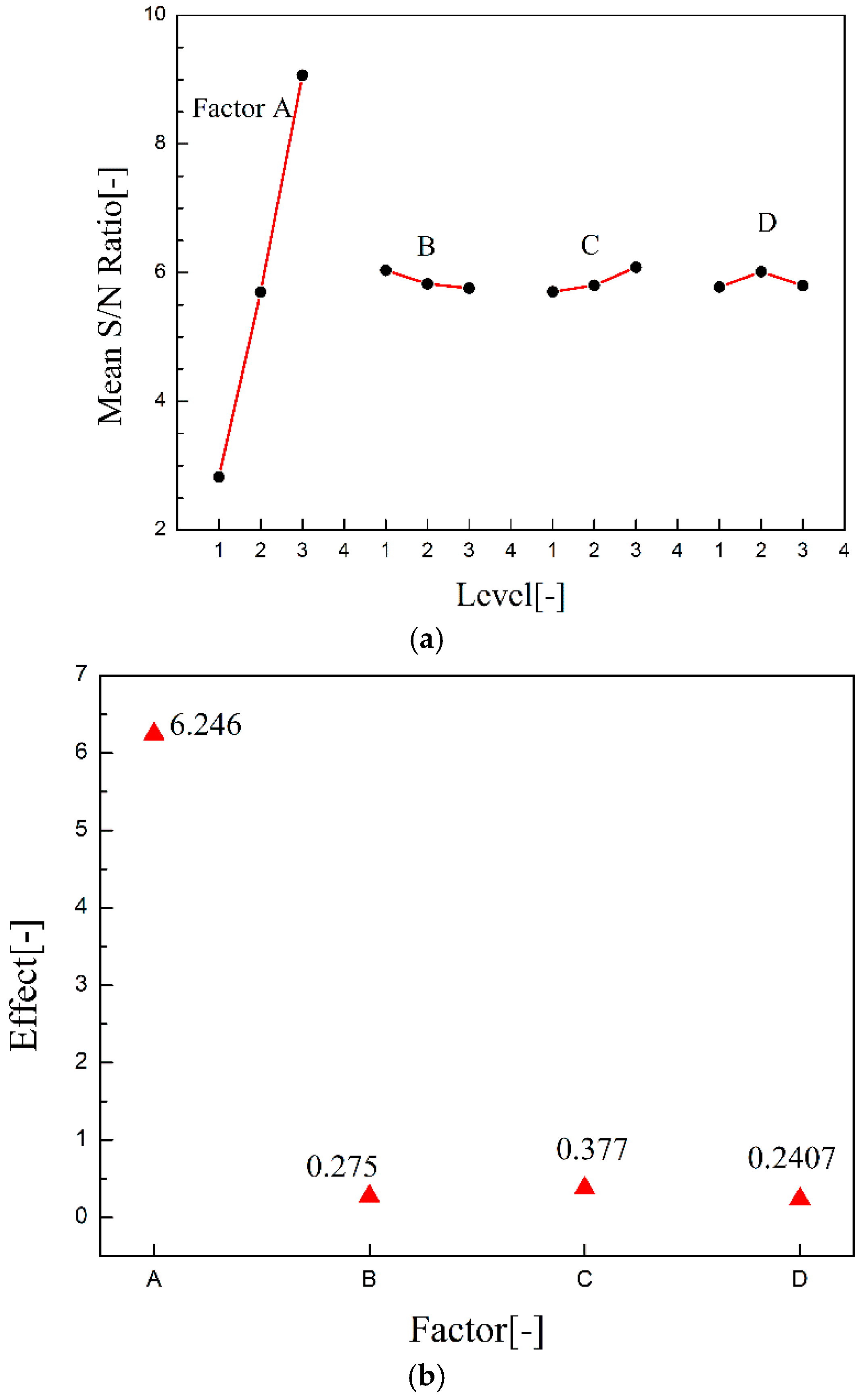
- In order to investigate the influence strength order of four factors (TSRs, α, TI, and ks/ds) to the wake effect of central rotating shaft on the performance of VAWT, the Taguchi method has been employed in this study, the analyses of signal-to-noise ratios (S/N ratios) suggest that the influence strength order of the factors is: TSRs > ks/ds > α > TI. In addition, the analysis of the S/N ratios also report that, within the range that we have analyzed in this current study, the operating conditions of TSR = 4, α = 5%, ks/ds = 1 × 10⁻², and TI = 8% can maximize the power coefficient of VAWT and the negative effect produced by the rotating shaft will be minimized. This conclusion provides reference for the optimum operating conditions of small VAWT in urban environment.
Author Contributions
Funding
Acknowledgments
Conflicts of Interest
Nomenclature
| A | Swept area of wind turbine (m2) |
| C | Length of chord line (m) |
| Cm | Instantaneous moment coefficient (-) |
| Cp | Power coefficient (-) |
| CoP | Pressure coefficient (-) |
| Fluctuation amplitude of lift coefficient of central shaft (-) | |
| Fluctuation amplitude of drag coefficient of central shaft (-) | |
| lift-drag coefficient ratio of central shaft (-) | |
| D | Diameter of wind turbine (m) |
| d | Cylinder diameter (m) |
| ds | Diameter of shaft (m) |
| Fl | Lift forces of central shaft (N) |
| Fd | Drag forces of central shaft (N) |
| H | Height of blade (m) |
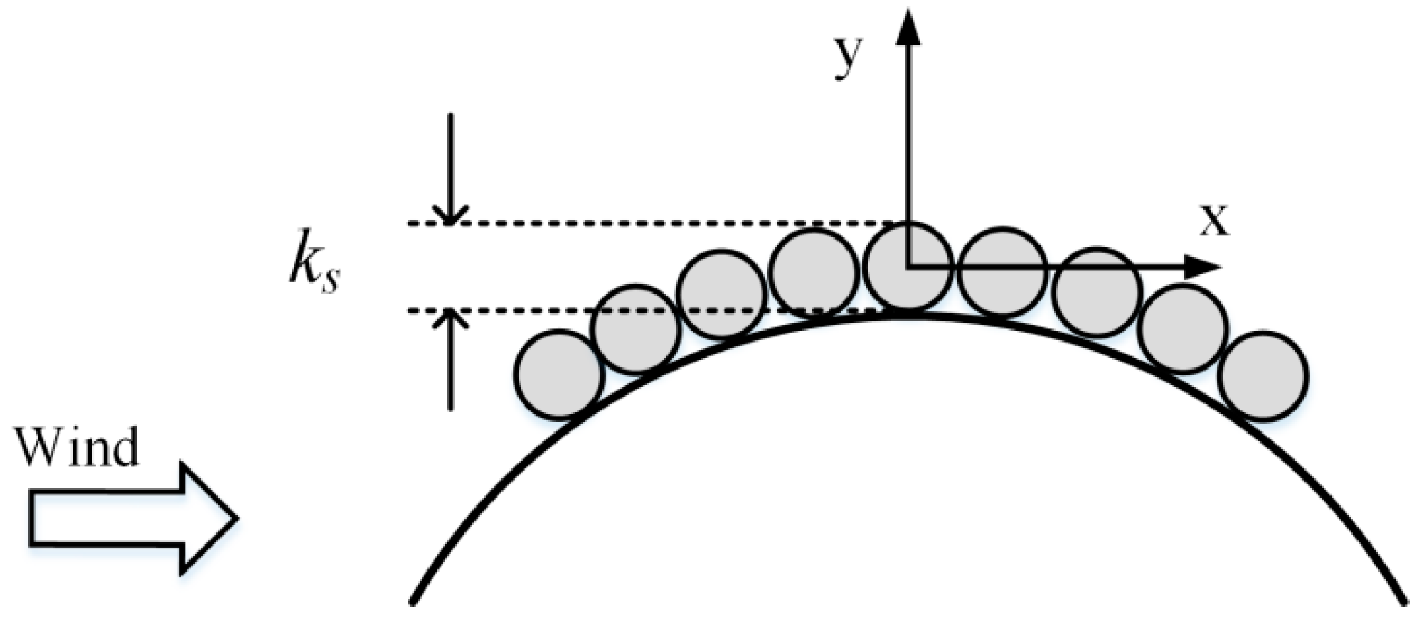
| ks | Roughness height of the shaft (m) |
| n | Number of blades (-) |
| R | Radius of wind turbine (m) |
| Res | Shaft diameter-based Reynolds number (-) |
| S/N ratio | Signal-noise ratio (-) |
| TI | Turbulence intensity (%) |
| U∞ | Free wind velocity [m/s] |
| y+ | Dimensionless wall distance (-) |
| α | Ratio of the shaft diameter to the wind turbine diameter (-) |
| θ | Azimuthal angle [°] |
| ω | Rotor angular velocity of the wind turbine (rad/s) |
| ρ | Air density (kg/m3) |
| CFD | Computational fluid dynamics |
| HAWT | Horizontal axis wind turbine |
| SST | Shear stress transport |
| TSR | Tip speed ratio |
| VAWT | Vertical axis wind turbine |
References
- Pagnini, L.C.; Burlando, M.; Repetto, M.P. Experimental power curve of small-size wind turbines in turbulent urban environment. Appl. Energy 2015, 154, 112–121. [Google Scholar] [CrossRef]
- Mabrouk, I.B.; Hami, A.E.; Walha, L.; Zghal, B.; Haddar, M. Dynamic vibrations in wind energy system: Application to vertical axis wind turbine. Mech. Syst. Signal Process. 2017, 85, 396–414. [Google Scholar] [CrossRef]
- Howell, R.; Qin, N.; Edwards, J.; Durrani, N. Wind tunnel and numerical study vertical axis wind turbine. Renew. Energy 2010, 35, 412–422. [Google Scholar] [CrossRef]
- Booker, J.D.; Mellor, P.H.; Wrbel, R.; Drury, D. A compact, high efficiency contra-rotating generator suitable for wind turbines in the urban environment. Renew. Energy 2010, 35, 2027–2033. [Google Scholar] [CrossRef]
- Islam, M.R.; Mekhilef, S.; Saidur, R. Process and recent trends of wind energy technology. Renew. Sustain. Energy Rev. 2013, 21, 456–468. [Google Scholar] [CrossRef]
- Islam, M.; Fartaj, A.; Carriveau, R. Analysis of design parameters related to a fixed-pitch straight-bladed vertical axis wind turbine. Wind Eng. 2008, 32, 491–507. [Google Scholar] [CrossRef]
- MacPhee, D.; Beyene, A. Recent advances in rotor design of vertical axis wind turbines. Wind Eng. 2012, 36, 647–666. [Google Scholar] [CrossRef]
- Elkhoury, M.; Kiwata, T.; Aoun, E. Experimental and numerical investigation of a three-dimensional vertical-axis wind turbine with variable-pitch. J. Wind Eng. Ind. Aerodyn. 2015, 139, 111–123. [Google Scholar] [CrossRef]
- Siddiqui, M.S.; Durrani, N.; Akhtar, I. Quantification of the effects of geometric approximations on the performance of a vertical axis wind turbine. Renew. Energy 2015, 74, 661–670. [Google Scholar] [CrossRef]
- Zamani, M.; Maghrebi, M.J.; Varedi, S.R. Starting torque improvement using J-shaped straight-bladed Darrieus vertical axis wind turbine by means of numerical simulation. Renew. Energy 2016, 95, 109–126. [Google Scholar] [CrossRef]
- Li, Q.; Maeda, T.; Kamada, Y.; Murata, J.; Kawabata, T.; Shimizu, K.; Ogasawara, T.; Nakai, A.; Kasuya, T. Wind tunnel and numerical study of a straight-bladed vertical axis wind turbine in three-dimensional analysis (Part I: For predicting aerodynamic loads and performance). Energy 2016, 106, 443–452. [Google Scholar] [CrossRef]
- Delafin, P.L.; Nishino, T.; Kolios, A.; Wang, L. Comparison of low-order aerodynamic models and RANS CFD for full scale 3D vertical axis wind turbines. Energy 2017, 109, 564–575. [Google Scholar] [CrossRef]
- Zhong, J.; Li, J.; Guo, P. Effects of leading-edge rod on dynamic stall performance of a wind turbine airfoil. Proc. Inst. Mech. Eng. Part A J. Power Energy 2017, 231, 753–769. [Google Scholar] [CrossRef]
- Zamani, M.; Nazari, S.; Moshizi, S.A.; Maghrebi, M.J. Three dimensional simulation of J-shaped Darrieus vertical axis wind turbine. Energy 2016, 116, 1243–1255. [Google Scholar] [CrossRef]
- Chen, W.; Chen, C.; Huang, C.; Hwang, C. Power output analysis and optimization of two straight-bladed vertical-axis wind turbines. Appl. Energy 2017, 185, 223–232. [Google Scholar] [CrossRef]
- Bouchereau, V.; Rowlands, H. Methods and techniques to help quality function deployment (QFD). Benchmarking Int. J. 2000, 7, 8–19. [Google Scholar] [CrossRef]
- Xie, S.; Archer, C.L.; Ghaisas, N.; Meneveau, C. Benefits of collocating vertical-axis and horizontal-axis wind turbines in large wind farm. Wind Energy 2017, 20, 45–62. [Google Scholar] [CrossRef]
- Cai, X.; Gu, R.; Pan, P.; Zhu, J. Unsteady aerodynamic simulation of a full-scale horizontal axis wind turbine using CFD methodology. Energy Convers. Manag. 2016, 112, 146–156. [Google Scholar] [CrossRef]
- Kim, H.; Lee, S.; Lee, S. Influence of blade-tower interaction in upwind-type horizontal axis wind turbines on aerodynamics. J. Mech. Sci. Technol. 2011, 25, 1351–1360. [Google Scholar] [CrossRef]
- Liu, X.; Lu, C.; Li, G.; Godbole, A.; Chen, Y. Effects of aerodynamic damping on the tower load of offshore horizontal axis wind turbines. Appl. Energy 2017, 204, 1101–1114. [Google Scholar] [CrossRef]
- Rezaeiha, A.; Kalkman, I.; Montazeri, H.; Blocken, B. Effect of the shaft on the aerodynamic performance of urban vertical axis wind turbines. Energy Convers. Manag. 2017, 149, 616–630. [Google Scholar] [CrossRef]
- Chigliaro, M. Effect of Shaft Diameter on Darrieus Wind Turbine Performance. Ph.D. Thesis, Facolt’ di ingegneria of Università Degli Studi di Padova, Veneto Padova, Italy, 2013. [Google Scholar]
- Danao, L.A.M. The influence of unsteady wind on the performance and aerodynamics of vertical axis wind turbines. Ph.D. Thesis, The University of Sheffield, Sheffield, UK, September 2012. [Google Scholar]
- Rezaeiha, A.; Kalkman, I.; Blocken, B. CFD simulation of a vertical axis wind turbine operating at a moderate tip speed ratio: Guidelines for minimum domain size and azimuthal increment. Renew. Energy 2017, 107, 373–385. [Google Scholar] [CrossRef]
- Balduzzi, F.; Bianchini, A.; Maleci, R.; Ferrara, G.; Ferrari, L. Critical issues in the CFD simulation of Darrieus wind turbines. Renew. Energy 2016, 85, 419–435. [Google Scholar] [CrossRef]
- Karbasian, H.R.; Kim, K.C. Numerical investigations on flow structure and behavior of vortices in the dynamic stall of an oscillating pitching hydrofoil. Ocean Eng. 2016, 127, 200–211. [Google Scholar] [CrossRef]
- Streiner, S.; Krämer, E.; Eulitz, A.; Armbruster, P. Aeroelastic analysis of wind turbines applying 3D CFD computational results. J. Phys. Conf. Ser. 2007, 75, 012015. [Google Scholar] [CrossRef] [Green Version]
- Wekesa, D.W.; Wang, C.; Wei, Y.; Kamau, J.N.; Danao, L.A. A numerical analysis of unsteady inflow wind for site specific vertical axis wind turbine: A case study for Marsabit and Garissa in Kenya. Renew. Energy 2015, 76, 648–661. [Google Scholar] [CrossRef]
- Danao, L.A.; Edwards, J.; Eboibi, O.; Howell, R. A numerical investigation into the influence of unsteady wind on the performance and aerodynamic of a vertical axis wind turbine. Appl. Energy 2014, 116, 111–124. [Google Scholar] [CrossRef]
- Menter, F.R.; Langtry, R.B.; Likki, S.R.; Suzen, Y.B.; Huang, P.G.; Völker, S. A correlation-based transition model using local variables-Part I: Model formulation. J. Turbomach. 2006, 128, 413–422. [Google Scholar] [CrossRef]
- George, J.; Owen, L.D.; Xing, T. Entropy generation in bypass transitional boundary layer flows. J. Hydrodyn. 2014, 26, 669–680. [Google Scholar] [CrossRef]
- Sørensen, N.N. CFD modeling of laminar-turbulent transition for airfoils and rotors using the γ- model. Wind Energy 2009, 12, 715–733. [Google Scholar] [CrossRef]
- Okamoto, T.; Yagita, M. The experimental investigation on the flow past a circular cylinder of finite length placed normal to the plane surface in a uniform stream. Bull. JSME 1973, 16, 805–814. [Google Scholar] [CrossRef]
- Norberg, C. An experimental investigation of the flow around a circular cylinder: Influence of aspect ratio. J. Fluid Mech. 1994, 258, 287–316. [Google Scholar] [CrossRef]
- Prsic, M.A.; Ong, M.C.; Pettersen, B.; Myrhaug, D. Large eddy simulations of flow around a smooth circular cylinder in a uniform current in the subcritical flow regime. Ocean Eng. 2014, 77, 61–73. [Google Scholar] [CrossRef]
- Gao, Y.; Zong, Z.; Zou, L.; Takagi, S.; Jiang, Z. Numerical simulation of vortex-induced vibration of a circular cylinder with different surface roughness. Mar. Struct. 2018, 57, 165–179. [Google Scholar] [CrossRef]
- Rodriguez, I.; Lehmkuhl, O.; Piomelli, U.; Chiva, J.; Borrell, R.; Oliva, A. LES-based study of the roughness effects on the wake of a circular cylinder from subcritical to transcritical Reynolds numbers. Flow Turbul. Combust. 2017, 99, 729–763. [Google Scholar] [CrossRef]
- Wekesa, D.W.; Wang, C.; Wei, Y.; Danao, L.A. Influence of operating conditions on unsteady wind performance of vertical axis wind turbines operating within a fluctuating free-stream: A numerical study. J. Wind Eng. Ind. Aerodyn. 2014, 135, 76–89. [Google Scholar] [CrossRef]
- Rezaeiha, A.; Montazeri, H.; Blocken, B. Towards accurate CFD simulations of vertical axis wind turbines at different tip speed ratios and solidities: Guidelines for azimuthal increment, domain size and convergence. Energy Convers. Manag. 2018, 156, 301–316. [Google Scholar] [CrossRef]
- Lardeau, S.; Leschziner, M.A. Unsteady RANS modeling of wake-blade interaction: Computational requirements and limitations. Comput. Fluids 2005, 34, 3–21. [Google Scholar] [CrossRef]
- D’Errico, J.R.; Zaino, N.A. Statistical tolerancing using a modification of Taguchi’s method. Technometrics 1988, 30, 397–405. [Google Scholar] [CrossRef]
- Wu, C.; Liang, W. Effects of geometry and injection-molding parameters on weld-line strength. Polym. Eng. Sci. 2005, 45, 1021–1030. [Google Scholar] [CrossRef]
- Tsui, K. An overview of Taguchi method and newly developed statistical methods for robust design. IIE Trans. 1992, 24, 44–57. [Google Scholar] [CrossRef]
- Yang, W.H.; Tarng, Y.S. Design optimization cutting parameters for turning operations based on the Taguchi method. J. Mater. Process. Technol. 1998, 84, 122–129. [Google Scholar] [CrossRef]
- Siddiqui, M.S.; Rasheed, A.; Kvamsdal, T.; Tabib, M. Effect of turbulence intensity on the performance of an offshore vertical axis wind turbine. Energy Procedia 2015, 80, 312–320. [Google Scholar] [CrossRef]
- Selvaraj, D.P.; Chandramohan, P.; Mohanraj, M. Optimization of surface roughness, cutting force and tool wear of nitrogen alloyed duplex stainless steel in a dry turning process using Taguchi method. Measurement 2014, 49, 205–215. [Google Scholar] [CrossRef]
- Chen, W.; Chen, C.; Hung, C. Taguchi approach for co-gasification optimization of torrefied biomass and coal. Bioresour. Technol. 2013, 144, 615–622. [Google Scholar] [CrossRef] [PubMed]
- Liao, C.; Kao, H. Supplier selection model using Taguchi loss function, analytical hierarchy process and multi-choice goal programming. Comput. Ind. Eng. 2017, 58, 571–577. [Google Scholar] [CrossRef]
- Canel, T.; Kaya, A.U.; Celik, B. Parameter optimization of nanosecond laser for microdrilling on PVC by Taguchi method. Opt. Laser Technol. 2012, 44, 2347–2353. [Google Scholar] [CrossRef]
- South, P.; Mitchell, R.; Jacobs, E. Strategies for the Evaluation of Advanced Wind Energy; SERI/SP-635-1142; Solar Energy Research Institute: Lakewood, CO, USA, 1983. [Google Scholar]
- Teymourtash, A.R.; Salimipour, S.E. Compressibility effects on the flow past a rotating cylinder. Phys. Fluids 2017, 29, 016101. [Google Scholar] [CrossRef]
- Kang, S.; Choi, H. Laminar flow past a rotating circular cylinder. Phys. Fluids 1999, 11, 3312–3321. [Google Scholar] [CrossRef]
- Parker, C.M.; Leftwich, M.C. The effect of tip speed ratio on a vertical axis wind turbine at high Reynolds numbers. Exp. Fluids 2016, 57, 74. [Google Scholar] [CrossRef]
- Möllerström, E.; Ottermo, F.; Goude, A.; Eriksson, S.; Hylander, J.; Bernhoff, H. Turbulence influence on wind energy extraction for a medium size vertical axis wind turbine. Wind Energy 2016, 19, 1963–1973. [Google Scholar] [CrossRef]


| Parameter | Value |
|---|---|
| Airfoil | NACA0022 |
| Number of blades, n | 3 |
| Chord length, (m) | 0.04 |
| Height of blade, (m) | 0.6 |
| Diameter of turbine, (m) | 0.7 |
| Diameter of shaft, (m) | 0.027 |
| Domain width, (m) | 14 |
| Domain length, (m) | 14 |
| Inner region diameter, (m) | 1.05 |
| Case | St | Errors Relative to Previous Experiment or Simulation |
|---|---|---|
| Present simulation, Re = 1.32 × 10⁴ | 0.2152 | - |
| Experiment of Okamoto [33], Re = 1.33 × 10⁴ | 0.21 | 2.5% |
| Experiment of Norberg [34], Re = 1.30 × 10⁴ | 0.20 | 7.6% |
| Simulation of Prsic [35], Re = 1.31 × 10⁴ | 0.20 | 7.6% |
| Details of the Node Setup and Metrics | Coarse | Medium | Fine |
|---|---|---|---|
| Number of cells on the blade | 110 | 190 | 390 |
| Number of cells on the interface | 100 | 160 | 320 |
| Number of cells on the inlet boundary | 100 | 200 | 400 |
| Total number of grid | 69,782 | 153,561 | 242,315 |
| Power coefficient of turbine | 0.2615 | 0.2797 | 0.2802 |
| Azimuthal angle of blade in one time step (°) | 0.25 | 0.5 | 1 |
| Time step (milliseconds) | 0.054541 | 0.109018 | 0.21817 |
| Number of time steps in one revolution | 1440 | 720 | 360 |
| Power coefficient | 0.2791 | 0.2797 | 0.2778 |
| Factor | Control Parameter | Notation | Level | ||
|---|---|---|---|---|---|
| 1 | 2 | 3 | |||
| A | Tip speed ratio | TSR | 2 | 3 | 4 |
| B | Shaft diameter to wind turbine diameter ratios | α | 5% | 7% | 9% |
| C | Relative surface roughness value of the shaft | ks/ds | 1 × 10⁻⁴ | 1 × 10⁻³ | 1 × 10⁻² |
| D | Turbulent intensity of incoming flow | TI | 4% | 8% | 12% |
| Run | Factor | |||
|---|---|---|---|---|
| A | B | C | D | |
| 1 | 1 | 1 | 1 | 1 |
| 2 | 1 | 2 | 2 | 2 |
| 3 | 1 | 3 | 3 | 3 |
| 4 | 2 | 1 | 2 | 3 |
| 5 | 2 | 2 | 3 | 1 |
| 6 | 2 | 3 | 1 | 2 |
| 7 | 3 | 1 | 3 | 2 |
| 8 | 3 | 2 | 1 | 3 |
| 9 | 3 | 3 | 2 | 1 |
| Run | Cp | S/N Ratio |
|---|---|---|
| 1 | −0.1359 | 2.747 |
| 2 | −0.1248 | 2.879 |
| 3 | −0.1278 | 2.844 |
| 4 | 0.07698 | 5.747 |
| 5 | 0.07965 | 5.792 |
| 6 | 0.06566 | 5.558 |
| 7 | 0.26224 | 9.610 |
| 8 | 0.23032 | 8.810 |
| 9 | 0.22933 | 8.786 |
© 2018 by the authors. Licensee MDPI, Basel, Switzerland. This article is an open access article distributed under the terms and conditions of the Creative Commons Attribution (CC BY) license (http://creativecommons.org/licenses/by/4.0/).
Share and Cite
Zhang, L.; Zhu, K.; Zhong, J.; Zhang, L.; Jiang, T.; Li, S.; Zhang, Z. Numerical Investigations of the Effects of the Rotating Shaft and Optimization of Urban Vertical Axis Wind Turbines. Energies 2018, 11, 1870. https://doi.org/10.3390/en11071870
Zhang L, Zhu K, Zhong J, Zhang L, Jiang T, Li S, Zhang Z. Numerical Investigations of the Effects of the Rotating Shaft and Optimization of Urban Vertical Axis Wind Turbines. Energies. 2018; 11(7):1870. https://doi.org/10.3390/en11071870
Chicago/Turabian StyleZhang, Lidong, Kaiqi Zhu, Junwei Zhong, Ling Zhang, Tieliu Jiang, Shaohua Li, and Zhongbin Zhang. 2018. "Numerical Investigations of the Effects of the Rotating Shaft and Optimization of Urban Vertical Axis Wind Turbines" Energies 11, no. 7: 1870. https://doi.org/10.3390/en11071870