A Methodology Based on Cyclostationary Analysis for Fault Detection of Hydraulic Axial Piston Pumps


Department of Engineering and Architecture, University of Parma, 43124 Parma, Italy
*
Author to whom correspondence should be addressed.
Energies 2018, 11(7), 1874; https://doi.org/10.3390/en11071874
Submission received: 14 June 2018
/
Revised: 11 July 2018
/
Accepted: 13 July 2018
/
Published: 18 July 2018
(This article belongs to the Special Issue Energy Efficiency and Controllability of Fluid Power Systems 2018)
Abstract
:Condition monitoring has been an active area of research in many industrial fields during the last decades, particularly in fluid power systems. This paper presents a solution for the fault diagnosis of a variable displacement axial-piston pump, which is a critical component in many hydraulic systems. The proposed methodology follows a data-driven approach including data acquisition and feature extraction and is based on the analysis of acceleration signals through the theory of cyclostationarity. An experimental campaign was carried out on a laboratory test bench with the pump in the flawless state and in faulty states. Different operating conditions were considered and each test was repeated several times in order to acquire a suitable population to verify data repeatability. Results showed the capability of the proposed approach of detecting a typical fault related to worn slippers. Future works will include tests in order to apply the approach to a wider set of faults and the development of a classifier for accurate fault identification.
1. Introduction
In the last decades, the online condition monitoring of systems and components have been acquiring more and more importance for industries in order to definitively quit time-based maintenance and turn to condition-based maintenance. The time-based preventive maintenance does not consider the actual health state of the system, but it follows a schedule for periodic inspections during which the system is stopped or its productivity is somehow reduced. Therefore, the inspections performed when the system did not require any maintenance led to a useless system downtime and consequent loss of productivity. Nowadays, the trend is to move from time-based maintenance to condition-based maintenance, where the inspections are performed only when they are effectively required. The implementation of condition-based maintenance relies on an effective prognostics and health management (PHM) system, whose function is to identify if and when maintenance action is required. For this reason, in the last years, the research in the field of PHM has been growing in many industrial applications, making PHM one of the hottest research topics in the engineering field. The adoption of PHM solutions can therefore lead to important advantages in terms of reliability, security, and productivity of the system. This effort is transversal and active in many fields, including for oil hydraulic circuits and components. The leading sectors in the hydraulic circuit PHM are those where a plant downtime can lead to huge money losses, for instance, oil and gas and chemical industries, and those where strong security issues are involved, such as in the hydraulic systems installed on aircrafts [1,2]. The PHM solutions can also be exploited to improve the reliability of hydraulic components, such as a hydraulic pump, which is the object of this paper. Both diagnostics and prognostics are essential tasks for the implementation of condition-based maintenance, but they have different objectives. The diagnostics aims at identifying the health state of the system and can be considered the first step for the prognostic process, which in turn aims at identifying the remaining useful life (RUL) of the system. Different methodologies and approaches for the diagnostic process have been proposed in many engineering fields and they can be separated into two main classes: data-driven approaches and model-based approaches [3]. In most applications, the development of a numerical model which can be exploited for diagnostics is a difficult task; therefore, data-driven approaches are preferred.
The calculation of the RUL of a mechanical system or component is a very difficult task because it requires the capacity of foreseeing the evolution of a fault in the future. Even in prognostics, a classification in model-based approaches and data-driven approaches can be made, with the former preferred in most applications, but the development of a fault growth model is extremely complex for most of the deteriorating mechanisms in mechanical systems.
The objective of diagnostics can be summarized in the expression: fault detection and identification (FDI), which is often used in the literature. Indeed, the diagnostics aim at detecting whether a fault is present in the system first (fault detection) and then at identifying which fault occurred (fault identification). Any diagnostic approach requires the acquisition of signals from the system and therefore requires the installation of a suitable set of sensors for the system monitoring. The acceleration signals convey a lot of information about the system’s healthy status and are currently used for the monitoring and diagnostics of different mechanical systems.
The acceleration signals are the result of excitations due to many sources: for example, in the case of an internal combustion engine [4,5], the acceleration signal acquired by means of an accelerometer installed on a precise position on the engine is caused by the gas combustion, the reciprocating motion of the pistons, the contacts’ forces in the cam mechanism, and so on. Therefore, the acquired acceleration signals contain contributions due to all these phenomena. From one end, the signal contains information which can be used for condition monitoring or diagnostic purposes, but on the other end, all these contributions are mixed together and therefore the information carried by the signal is difficult to interpret; therefore, a preprocessing of the raw signal is needed to extract features which are related to the machine faults.
Furthermore, the use of accelerometers is the standard for the monitoring and the diagnostics of bearings [6,7] that are present in any roto-dynamic machine and also in centrifugal and positive displacement pumps. Acceleration signals have also been exploited for the detection of cavitation in centrifugal and gerotor pumps [8,9]; for this purpose, noise measurements have also often been considered [10,11].
The vibration of hydraulic pumps, which can be measured using accelerometers installed on the pump case, is affected by the majority of the faults, and therefore it is considered in many works which propose diagnostics solutions for hydraulic pumps [12,13,14,15,16]. Other works about condition monitoring exploit vibration signals to train neural networks and compute the diagnosis [17,18,19]. Besides the acceleration of the pump case, another important signal which is affected by the faults and can be used for the development of an effective diagnostic algorithm is the delivery pressure signal [20,21,22,23]. The delivery pressure can be measured by means of cheaper sensors, but it can detect only faults that involve the fluid dynamics of the system. Temperature signals have also been exploited for the monitoring of hydraulic pumps. The differential temperature between inlet and outlet ports can be used to compute the overall efficiency for the evaluation of the machine performance. This method has been applied to an external gear pump [24] and to a variable displacement axial-piston pump with external drainage [25]. The approach is not suitable when the pump operating conditions change rapidly because the efficiency measurements are affected by the time constant of the temperature sensors; its application is limited to stationary conditions.
This paper presents a methodology for the analysis of acceleration signals and demonstrates its application for the diagnostics of a variable displacement axial-piston pump. This methodology relies on the theory of cyclostationarity. This approach has been proposed in the literature: in [26], the theory of cyclostationarity has been applied in order to discriminate the different sources of signal in helicopter gearboxes, such as gear signals, which are purely periodic, and bearing signals, which highlight some randomness and which are approximately second-order cyclostationary; how cyclostationarity can be exploited in machine diagnostics and the separation of different mechanical sources is demonstrated in [27]. Following the theory of cyclostationarity, the proposed methodology decomposes the acceleration signal in its periodic first-order cyclostationary (CS1) and second-order cyclostationary (CS2) components. These two parts contain information about different phenomena and need to be separated and processed with different tools. This decomposition of the signal is connected with the field of blind source separation (BSS), which aims at extracting all the independent sources from the analysis of the output measurements. The independent sources are the different excitation forces, while the output measurements are the accelerations signals acquired in different positions and directions. The objective of BSS is ambitious in the case of mechanical systems because there are many sources and their number is hardly known; a list of difficulties for the application of BSS techniques in the field of mechanical systems can be found in [28]. However, in many applications, the complete knowledge of the sources is not required and the ambition of the BSS can be reduced; instead of extracting the set of independent sources, the contribution of any source could be extracted by introducing the concept known in the literature as blind component separation (BCS) or blind signal extraction (BSE) [29].
The methodology proposed in this work for the separation of the different components of an acceleration signal follows the general guideline proposed by Antoni in [30]. The methodology is then applied on experimental signals acquired from two accelerometers installed on the pump case. The experiments were carried out in healthy and faulty conditions; the faulty condition was created by introducing artificially worn piston slippers within the pump. The results show that the proposed methodology for the analysis of the acceleration signals can extract features which highlight the presence of the considered fault.
2. Data Preprocessing and Analysis Procedure
A generic acceleration signal is decomposed into three main components as illustrated in Equation (1):
- is the predictable part of the signal: the CS1 part, i.e., the periodic part of the signal;
- is the CS2 part of the signal defined over the set of cyclic frequencies of interest;
- is the remaining noise which contains the contributions which are not of interest, or anyway which are not included in or in . This part can also contain CS2 contributions which are related to cyclic frequencies not included in the set .
The proposed decomposition scheme is particularly suitable for the analysis of acceleration signals; Equation (1) is also a valid scheme for modelling acceleration signals. Only the CS1 and the CS2 components are considered because they are the most relevant in acceleration signals; the contribution at higher orders are usually negligible. The three components contain the contributions of different sources; for example, in rotating machines, the periodic component is usually linked to imbalances, misalignments, eccentricities, etc., while the CS2 part is due to other phenomena such as wear, friction forces, fluid turbulence, etc. A typical example is that of the gearbox [26,30], where the contributions due to the gear meshing are CS1 and therefore included in , while the contributions due to the ball bearings are CS2 and therefore included in .
The application of the proposed methodology allows the separation of different contributions which can be analyzed with most suitable tools. In particular, the periodic part of the signal can be effectively analyzed with the classical Fourier spectrum and do not need advanced cyclostationary tools. The CS2 part instead can be analyzed with the CS2 tools (cyclic modulation spectrum, spectral correlation density, and cyclic spectral coherence). The separation of the different parts is also important so as to eliminate the mutual interferences which can cause misleading results. In particular, it is a key point to extract the predictable part before analyzing the CS2 part [28].
The extraction of the predictable part of the acceleration signal consists in extracting its periodic part (CS1 part). The predictable part of the signal corresponds to its expected value:
where the expected value operator refers to the ensemble average and not to the time average. The ensemble average is computed by averaging different repetitions of the same stochastic process. Since the expected value is the periodic part of the signal, it can be computed through the operator , which extracts all the periodic components of the signal under the hypothesis of cycloergodicity. The property of cycloergodicity for cyclostationary signals is equivalent to ergodicity for stationary processes; therefore, for a cyclostationary and cycloergodic signal , the ensemble average is equivalent to the infinite cycle average [28]:
where is the cycle length and is the number of considered cycles. This formulation extracts only the periodic components which are multiples of the cycle, which needs to be known a priori. In the case of the hydraulic pump considered in this work, the basic cycle corresponds to one shaft revolution. In general, for rotating machines, the basic cycle can be calculated considering the kinematics of the machine.
The simplest and most adopted technique for the calculation of an estimate of the predictable part is the synchronous average (SA) [28,31]. Given a signal of finite-length L corresponding to cycles of samples each, the SA is expressed by Equation (4):
where the variable resets at the end of each cycle and is constrained in the range :
Basically, the SA is the cycle average computed on a finite number of cycles (this is always the case for actual signals). An equivalent expression in the frequency domain [30] is reported in Equation (6):
Equation (4) shows that the SA permits extraction of the predictable part at frequencies which are integer multiples of the cycle. The mathematical implementation of the SA is simple, but it faces some practical problems. Both formulations require an extremely precise estimation of the cycle length and both require and to be integers; furthermore, Equation (4) also requires to be an integer. All these conditions are easily satisfied if the acceleration signal is acquired with an angular sampling; in this case, is an integer and is also known exactly since it depends on the acquisition system. If a time sampling is adopted, in general, N is not an integer and needs to be estimated since it depends on the sampling frequency and the machine angular velocity. Some angular resampling techniques [32] are available to make an integer and use Equation (4) to compute the SA. These techniques require a tachometer for order tracking to correct speed fluctuations in the signal of at least one sample per cycle. However, a tachometric signal is not always available. Some attempts of computing the angular resampling without a tachometric signal have been done [33,34], but the obtained results showed some limitations in comparison to classical angular resampling techniques.
It is important to note that in rotating machines, the acceleration signals are theoretically cyclostationary in the angular domain and not in the time domain. Indeed, the phenomena which excite the output signal are cyclic with reference to the angular position and not necessarily to the time variable. This point becomes particularly important when the machine angular velocity is not perfectly constant over time, but it experiences some fluctuations. For this reason, an angular sampling, or an angular resampling, is required for a proper analysis of machine signals.
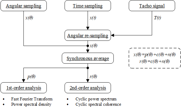
The proposed procedure decomposes the acquired signal into several components which need to be analyzed with the proper tools. A block diagram of the proposed procedure is reported in Figure 1. The first step of the procedure consists in obtaining an acceleration signal , a function of the angular position . The signal can be directly obtained through an angular sampling if a relative encoder is available to drive the acquisition. If the use of an encoder is not feasible, the time sampling of the acceleration signal is simpler to perform. The signal in the angular domain can be obtained through the application of one of the angular resampling procedures presented in [31]; these procedures require the availability of a tacho signal . The tacho signal could just be a signal with one impulse per revolution or it could consist of multiple impulses per revolution; the greater the number of impulses and the better the sampling will reduce the errors, due to the angular velocity variation within each revolution.
Once the signal in the angular domain is available, the synchronous average can be extracted with the algorithm presented in the previous section. The SA contains the CS1 components of the signal and therefore must be analyzed with the standard tools for the frequency analysis, such as the Fast Fourier Transform (FFT) or the Power Spectral Density (PSD). The residual signal can be computed by subtracting the SA from the acceleration signal . The residual signal contains the CS2 components and the higher-order cyclostationary components of the signal. The CS2 components can be analyzed through the tools presented in the previous section, such as the Spectral Correlation Density (SCD) and the Cyclic Spectral Coherence (CSC). It is important to subtract the SA before executing the analysis of the CS2 components, because the presence of periodic components could alter the results of the CS2 analysis. The residual signal also contains the background noise, which could make the results of the CS2 analysis less clear. The results presented concerning the CS2 analysis (e.g., Figure 12) appear clear without significative dispersion (grey area).
This analysis procedure allows one to separate the effects of different sources and analyze them, reducing the interferences [6,7]. Indeed, different faults induce different effects; for example, some faults could induce a modification of the periodic part of the signal, evident from the CS1 analysis, while other faults could induce a different power modulation of the signal, evident from the CS2 analysis.
3. Experimental Activity
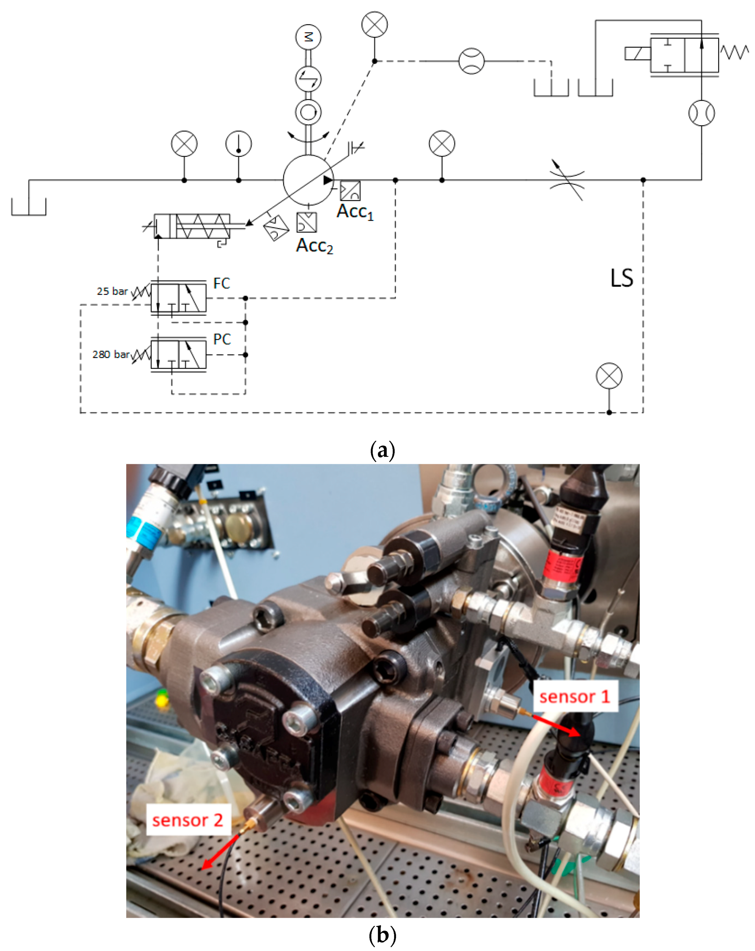
The methodology proposed in the previous section for the analysis of accelerations signal was applied on the data collected from two accelerometers installed on a variable displacement axial-piston pump. The pump was tested both in healthy and faulty conditions, and the final goal of the analysis was to extract suitable parameters for the pump diagnostics. This section presents the experimental layout and the experimental tests. The hydraulic pump considered in this activity is an axial-piston swash plate type with a maximum displacement of 84 cm3, produced by Casappa S.p.A® (Parma, Italy). The pump was equipped with a Flow Compensator (FC) and a Pressure Compensator (PC) and was tested in a load-sensing (LS) configuration; the hydraulic scheme of the experimental layout is reported in Figure 2a. All the tests carried out were executed on the test bench of the laboratory within the Engineering and Architectural Department of the University of Parma.
Two piezoelectric accelerometers (Acc1 and Acc2) were installed on the pump case as illustrated in Figure 2b and placed in orthogonal directions to understand which position provides the most relevant information.
As shown in Figure 2b, the first accelerometer (sensor 1) was installed on the angular sensor of the pump, which measures the angular position of the swash plate; this accelerometer measures the acceleration in the direction of the suction-delivery flow. The second accelerometer (sensor 2) is installed on the cover of the pump and measures the acceleration in the direction of the piston’s axis. Both accelerometers are the Brüel and Kjær type 4370 with a bandwidth up to 10 kHz and a maximum continuous sinusoidal acceleration of 20,000 m/s2.
The acquisitions were performed using a relative encoder for the angular sampling. The relative encoder counts 3600 steps per revolution, corresponding to an angular resolution of 0.1 deg. The angular resolution of the relative encoder leads to very high sampling frequencies when the pump is operated at the most common operating conditions; for example, at 2000 r/min, the sampling frequency is 120,000 kHz. This sampling frequency is much higher than the frequency required to exploit the accelerometer’s bandwidth.
The pump was tested in flawless and faulty conditions. The faulty condition was obtained by introducing artificially worn slippers in the flawless pump, replicating a common fault that occurs when the pump works in heavy working conditions for a long time. The dimensions of these worn slippers are equal to real worn slippers; with this procedure, in the future, the wear could be increased by machining the slipper. As suggested by the manufacturer, the worn slipper installed can be considered as an incipient fault, since the pump functioning was apparently the same as that of the flawless pump and the measured overall efficiency was unchanged.
The geometrical variations of the worn slippers can excite the pump case, inducing different vibrations. The flawless condition and the faulty condition were tested in the four operating conditions reported in Table 1, with the swash plate angle corresponding to about half displacement. The considered operating conditions are typical for this kind of pump.
For each acquisition, 900,000 samples, corresponding to 250 revolutions, were acquired. The tests were repeated 10 times for each operating condition in order to assess the repeatability of the acquisitions and extract robust features for the fault identification.
4. Experimental Data Analysis and Assessment
The objective of this section is to show how the proposed methodology for the analysis of acceleration signals can be used to identify the considered fault. In order to reduce the amount of data presented, only tests at 1500 r/min and 150 bar for both sensors are shown in detail, in addition to results for sensor 2 at 2000 r/min, which are reported in Section 4.3.
4.1. First-Order Analysis (Time Domain)
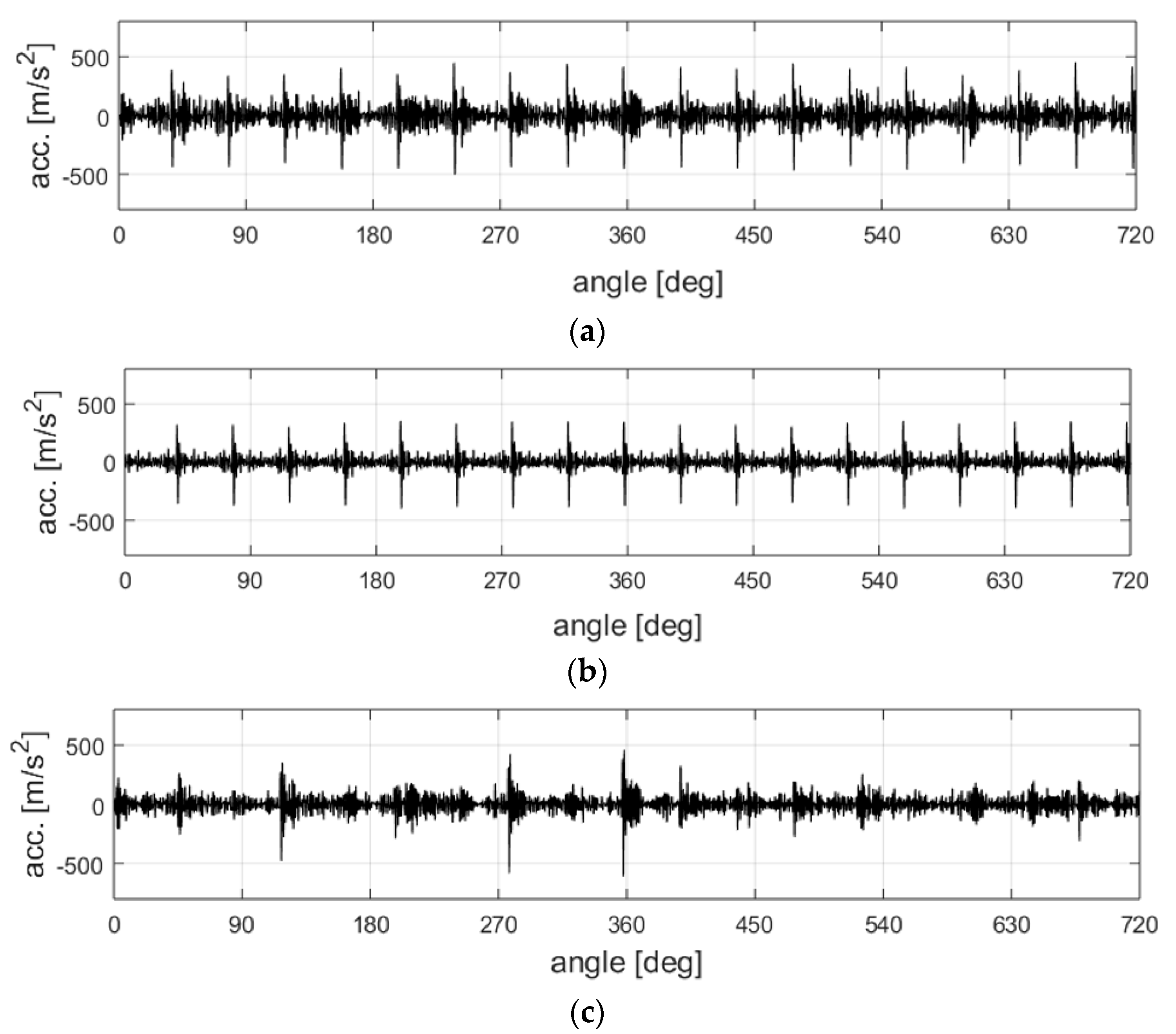
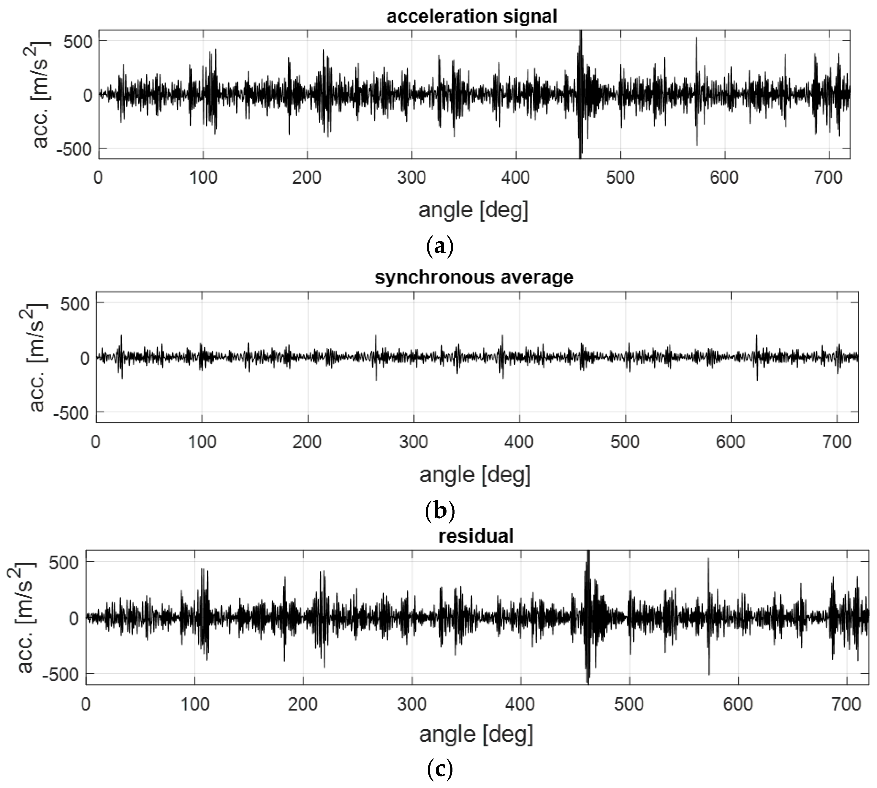
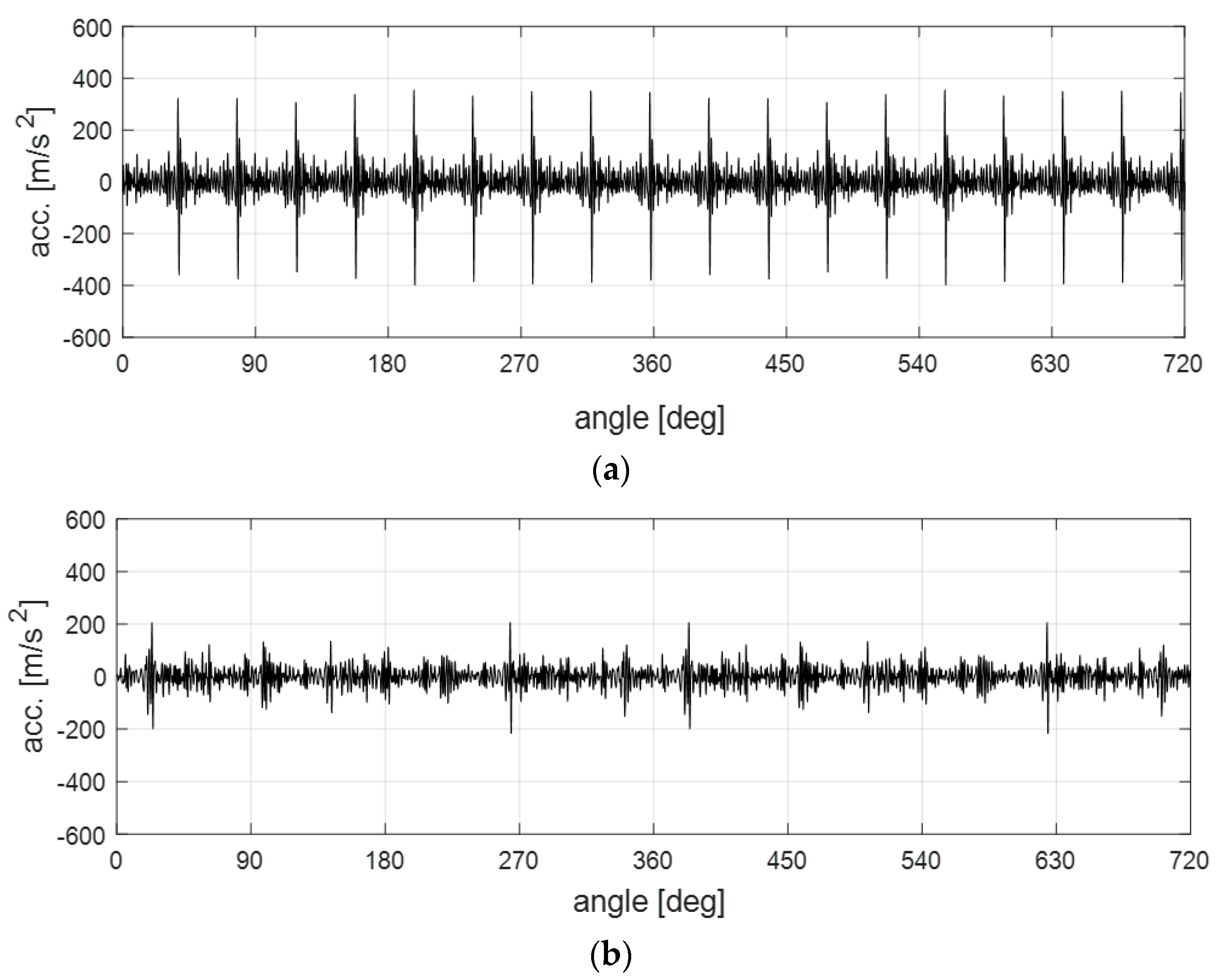
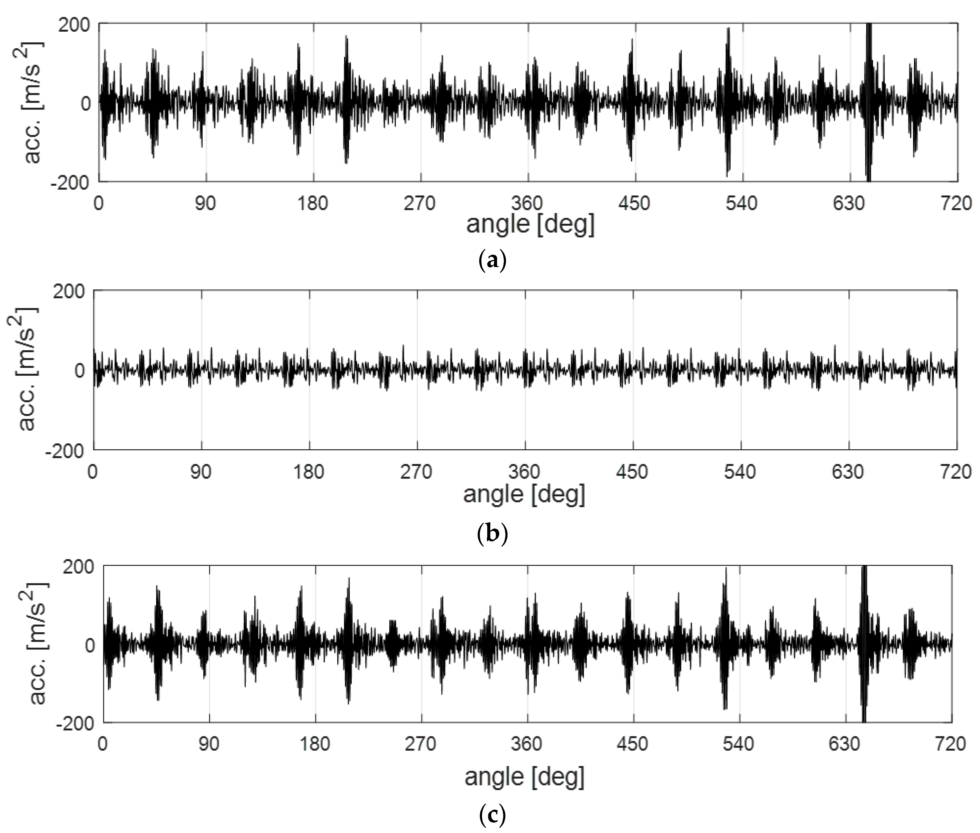
The first step of the proposed methodology consists of the calculation of the SA to extract the CS1 components from the raw signal; the SA has been calculated with 900,000 samples, corresponding to 250 revolutions. The residual signal, obtained by subtracting the SA from the raw signal, contains pure CS2 and higher-order components. Figure 3 and Figure 4 report the raw signal, the SA, and the residual signal for the signal acquired with sensor 1 in the case of the flawless pump and faulty pump, respectively; the signals are reported over a period of two revolutions (720 deg).
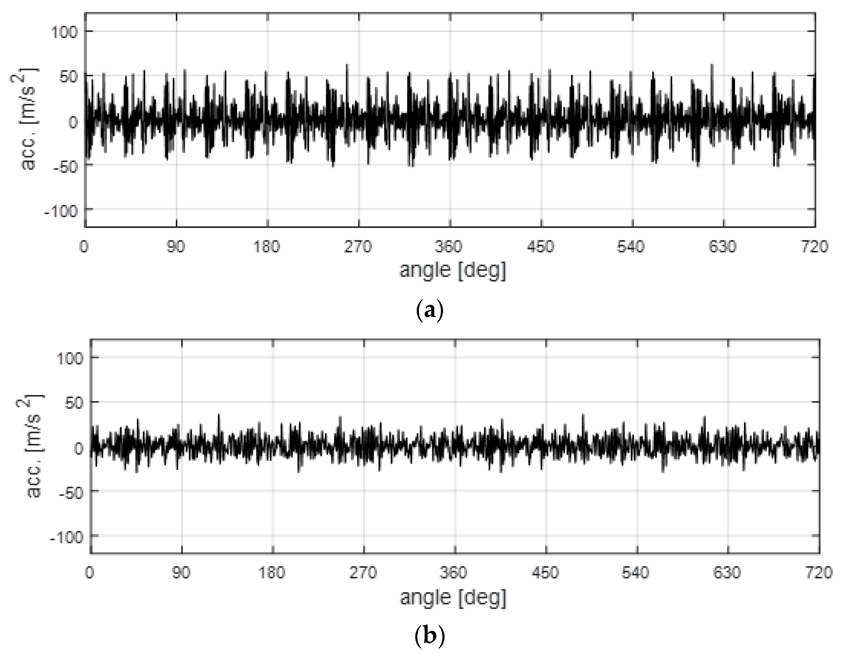
The SA is a cycle average and is repeated two times to cover the period of 720 deg. The SA shows a clear periodic behavior at the piston frequency (9 impulses per revolution). The residual signal collects the random part of the signal and does not show any repeatable behavior. A comparison of the SAs of the signals acquired from sensor 1 with the pump in healthy and faulty conditions is reported in Figure 5.
The SA signals for the flawless pump show a clear periodic behavior at the piston frequency. The SA for the faulty pump, i.e., with artificially worn slippers, does not show any remarkable periodic behavior at the piston frequency and seems to be random. From this first result, the analysis of the SA of sensor 1 seems to be effective for the identification of the fault.
Figure 6 reports the raw signal, the SA, and the residual signal for the signal acquired with sensor 2 in the case of the flawless pump. In this case, the shape of the SA does not show the impulses at the piston frequency found in Figure 4 for sensor 1.
The comparison among the SAs of the flawless pump and the faulty pump for the signals acquired with sensor 2 is reported in Figure 7. Also, in this case, the SA signals of the flawless pump show a periodic behavior at the piston frequency, while the SA of the faulty pump seems to be more random. The analysis of the signals in the angle domain showed some differences; however, the tools presented will be applied to highlight the differences between the flawless and faulty case.
4.2. First-Order Analysis (Frequency Domain)
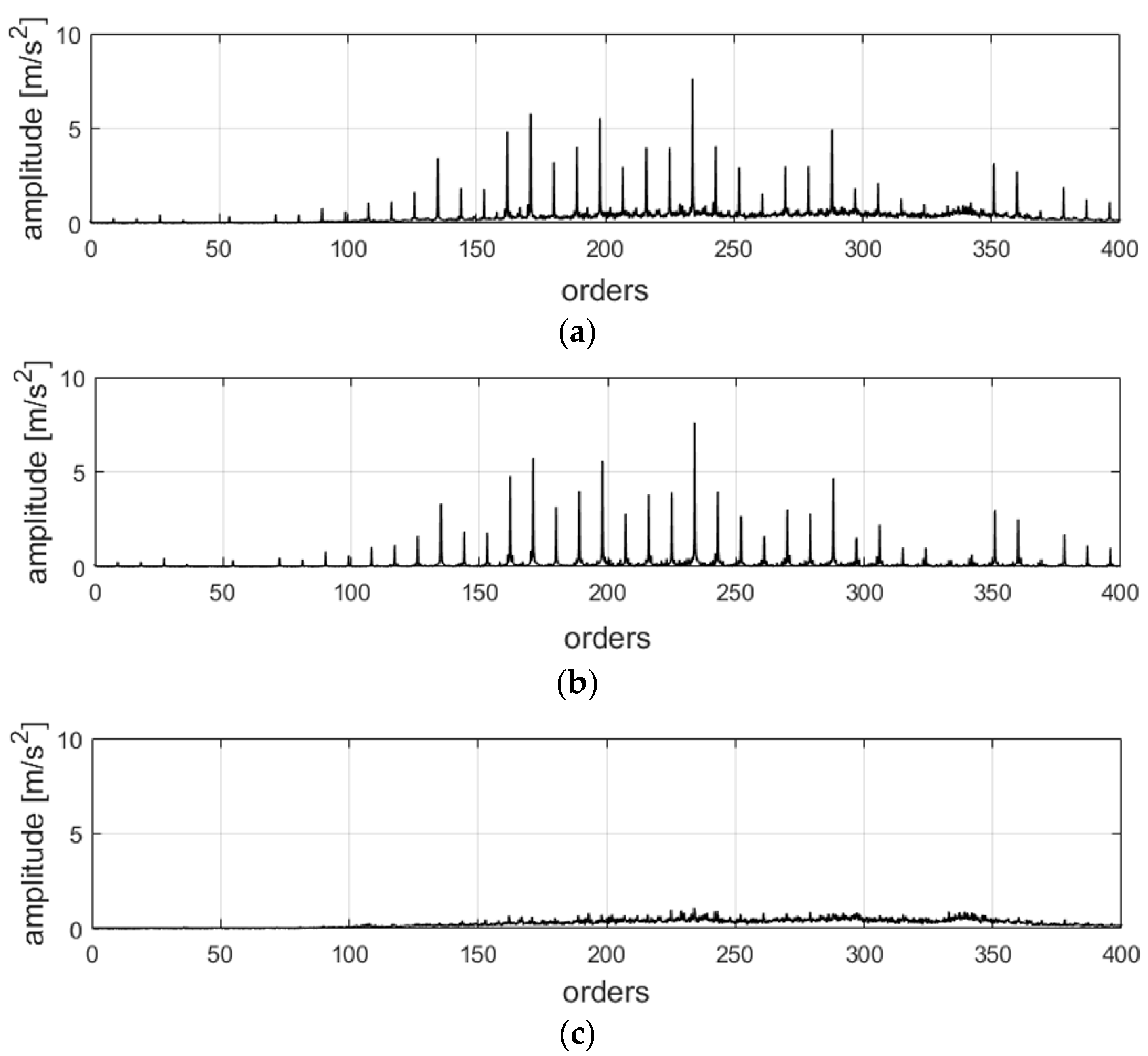
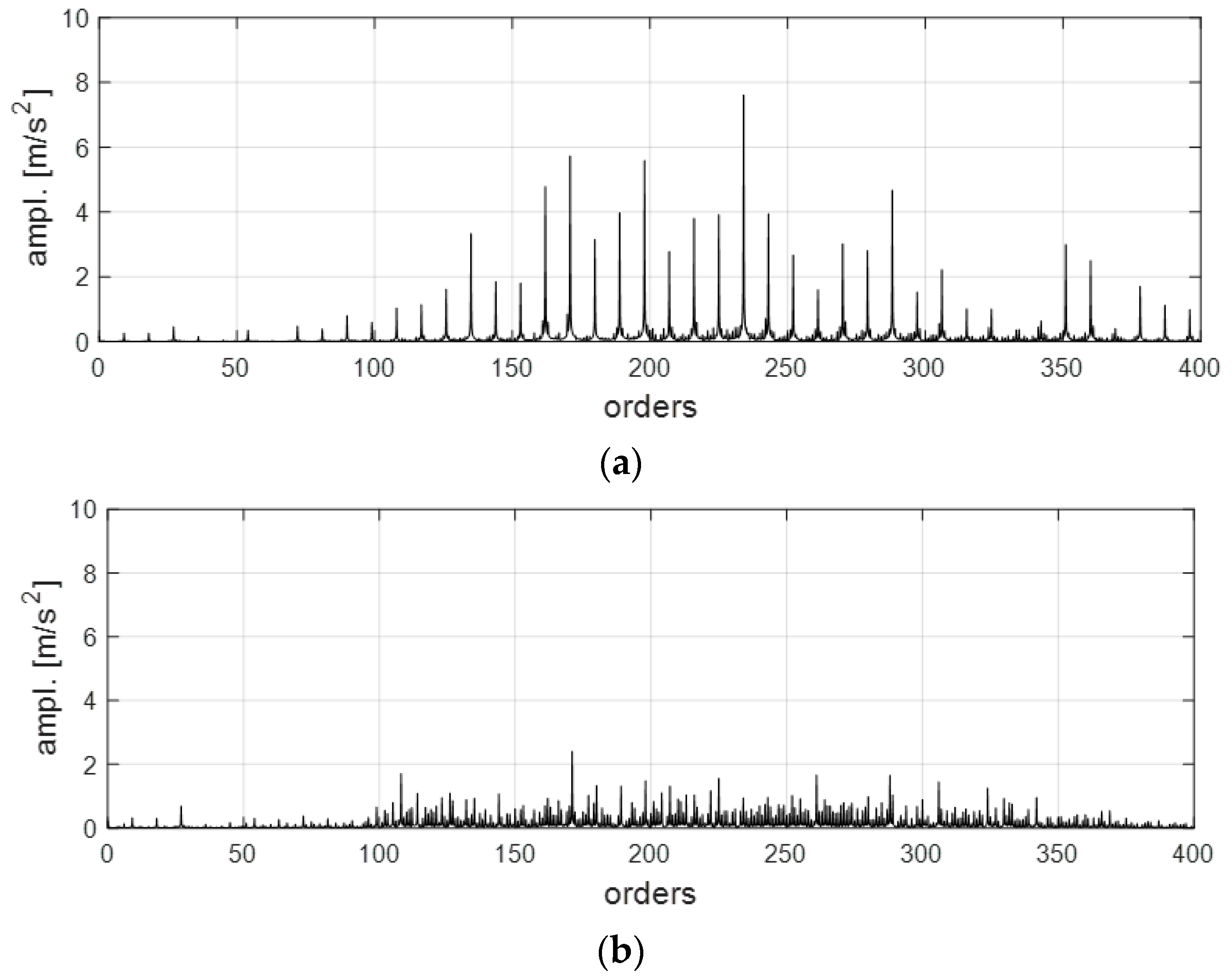
The first-order analysis in the frequency domain is performed by computing the FFT of the SA and the residual signals. Figure 8 highlights the FFT of the signals shown in Figure 3. The FFTs are reported up to order 400, which corresponds to the higher limit of the bandwidth of the accelerometers (10 kHz); order 1 corresponds to the shaft frequency and order 9 to the piston frequency. The SA collects all the periodic components and the residual signal remains completely random; the CS2, or higher-order, components are not highlighted by the FFT. The peaks in the FFT of the raw signal are the same of the FFT of the SA; these peaks are at order 9 and at its multiples.
A comparison of the FFTs of the SAs with the pump in healthy and faulty conditions for the signals acquired with sensor 1 is reported in Figure 9. The SA of the faulty pump does not show remarkable periodic components and looks random. This result confirms the result found in the analysis of the SA signals in the angle domain, as shown in Figure 7.
The acceleration signal acquired from sensor 1 loses its periodic components in the case of the faulty pump. This result is very important because it allows the identification of the fault related to worn slippers, which is one of the most common faults occurring in swash-plate-type pumps. This result can be explained looking at Figure 5, which reports the comparison between the healthy and the worn slippers. The slippers of the healthy case have a very similar height, while the slippers of the faulty case present different levels of wear and, in particular, different heights. In the healthy case, the slippers excite the pump vibration in the same way, leading to high harmonics at order 9 and its multiples. In the faulty case, the slippers excite the pump vibration in different ways; therefore, the harmonic at order 9 and its multiples reduce their intensity and the energy is distributed over the set of harmonics at multiples of order 1, i.e., the shaft frequency.
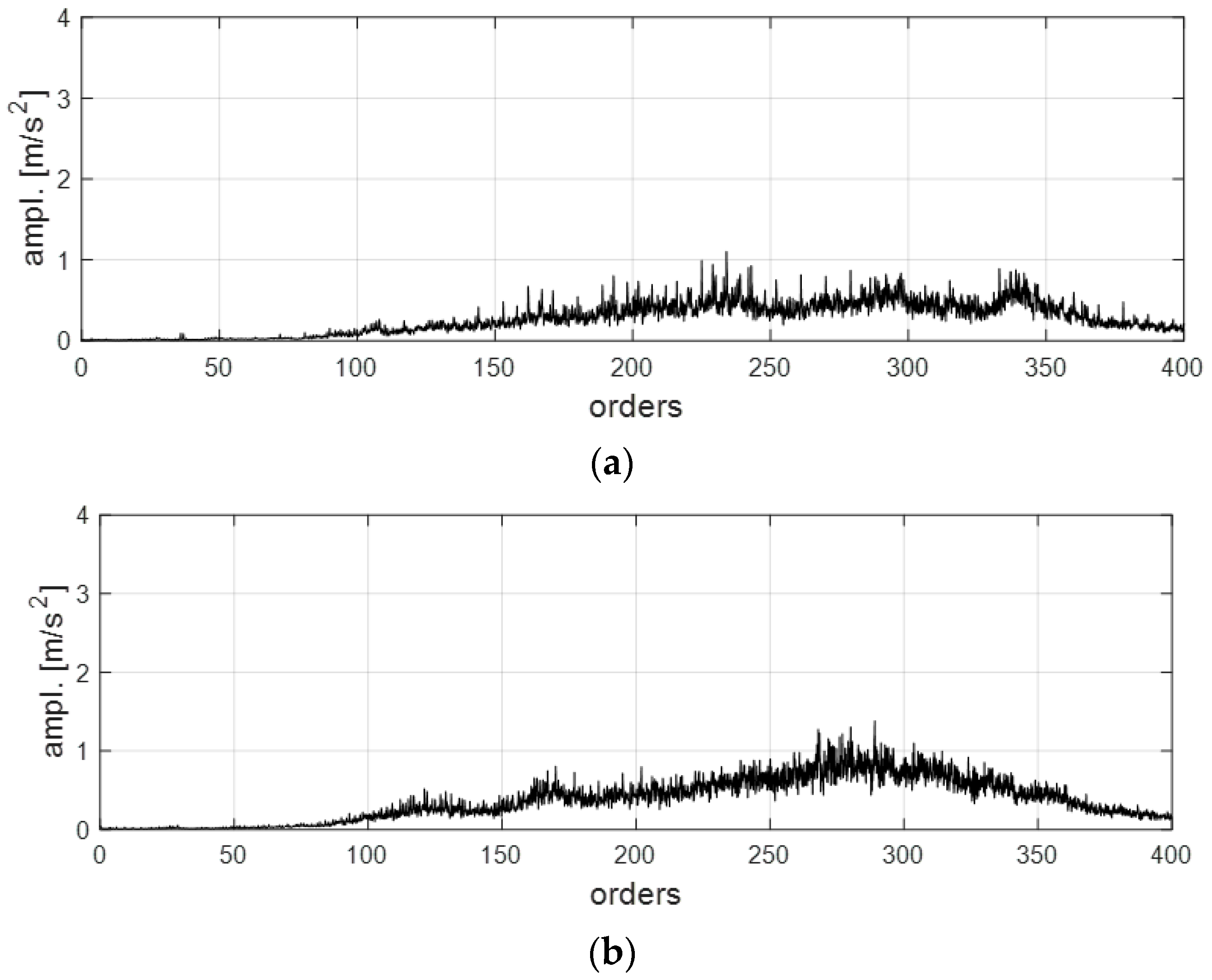
Figure 10 reports the FFTs of the residual signals. The residual signals in the flawless case and in the faulty cases are random since the periodic part was extracted by the SA.
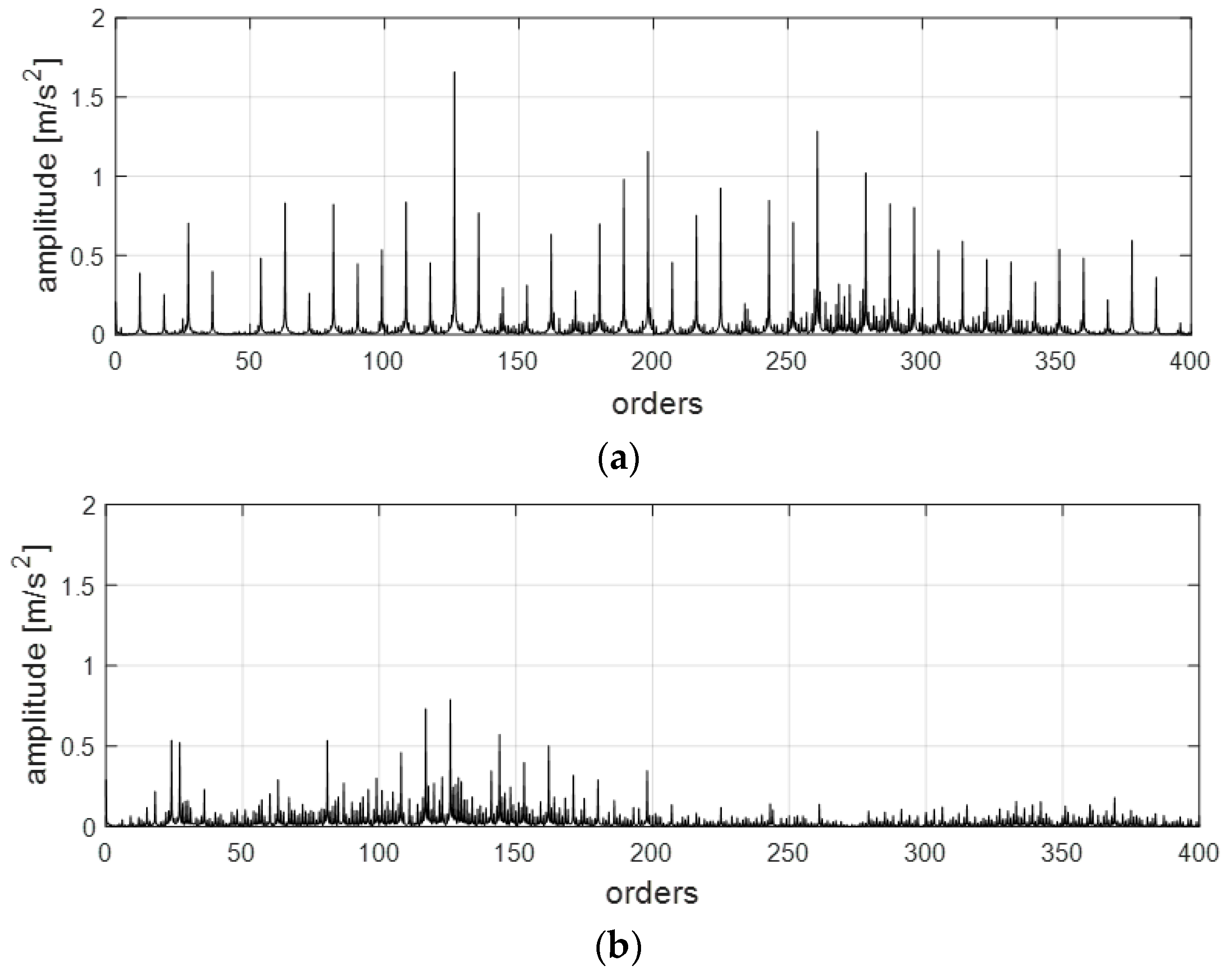
A comparison of the FFTs of the SA with the pump in healthy and faulty conditions for the signals acquired with sensor 2 is reported in Figure 11. The result highlighted in Figure 9 for sensor 1 is confirmed also for the signals acquired with sensor 2. In case of worn slippers, the harmonics at order 9 and at order 18 are remarkable and comparable to the ones found in case of flawless pump; at higher frequencies, the harmonics at multiples of order 9 are not evident and become comparable to the harmonics at multiples of order 1.
4.3. Second-Order Analysis
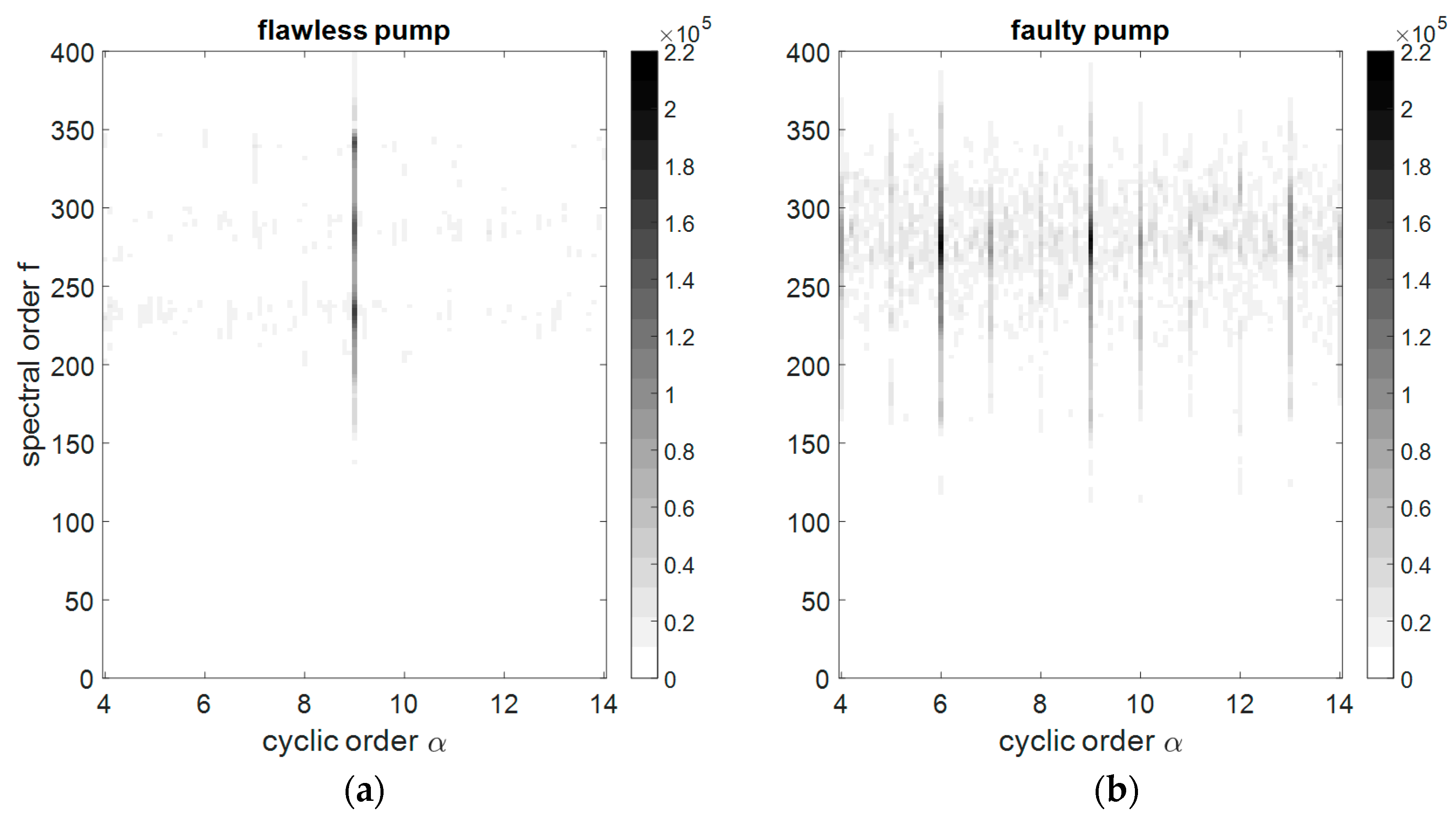
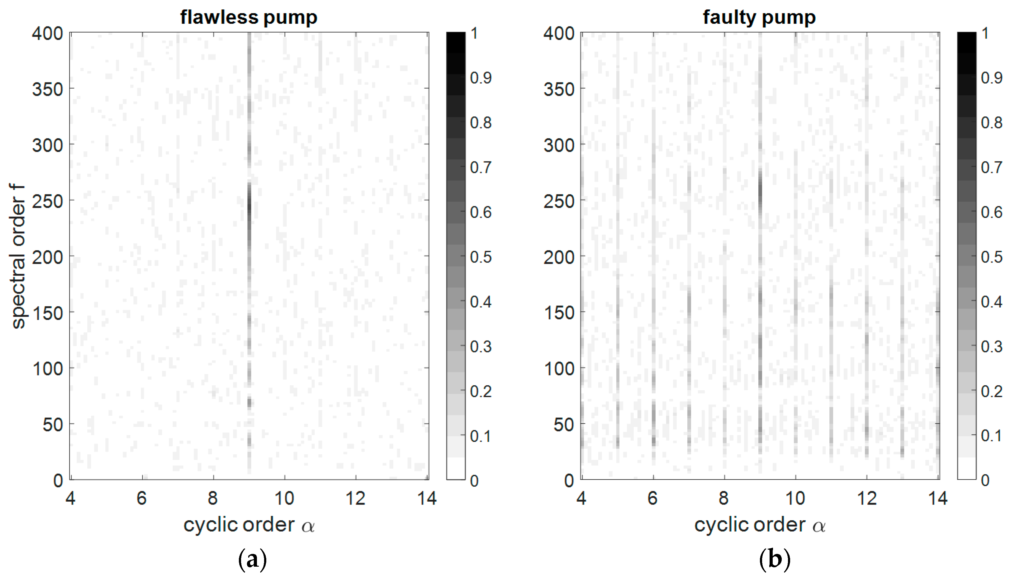
The CS2 analysis is performed by computing the spectral correlation density and the cyclic spectral coherence of the residual signals. The SCD highlights at which frequencies (orders in the angle domain) the signal power is modulated. The CSC is a normalized index that can be considered a measure of the degree of second-order cyclostationarity. Both these tools were calculated considering a signal length of 36,000 samples, corresponding to 10 revolutions, and a window length of 720 samples. With these parameters, the resulting resolutions are 0.1 orders for the cyclic frequency and 2.5 orders for the spectral frequency. Since the principal cyclic phenomenon is the one related to the pistons, only the cyclic frequencies around order 9 were considered to reduce the computational time.
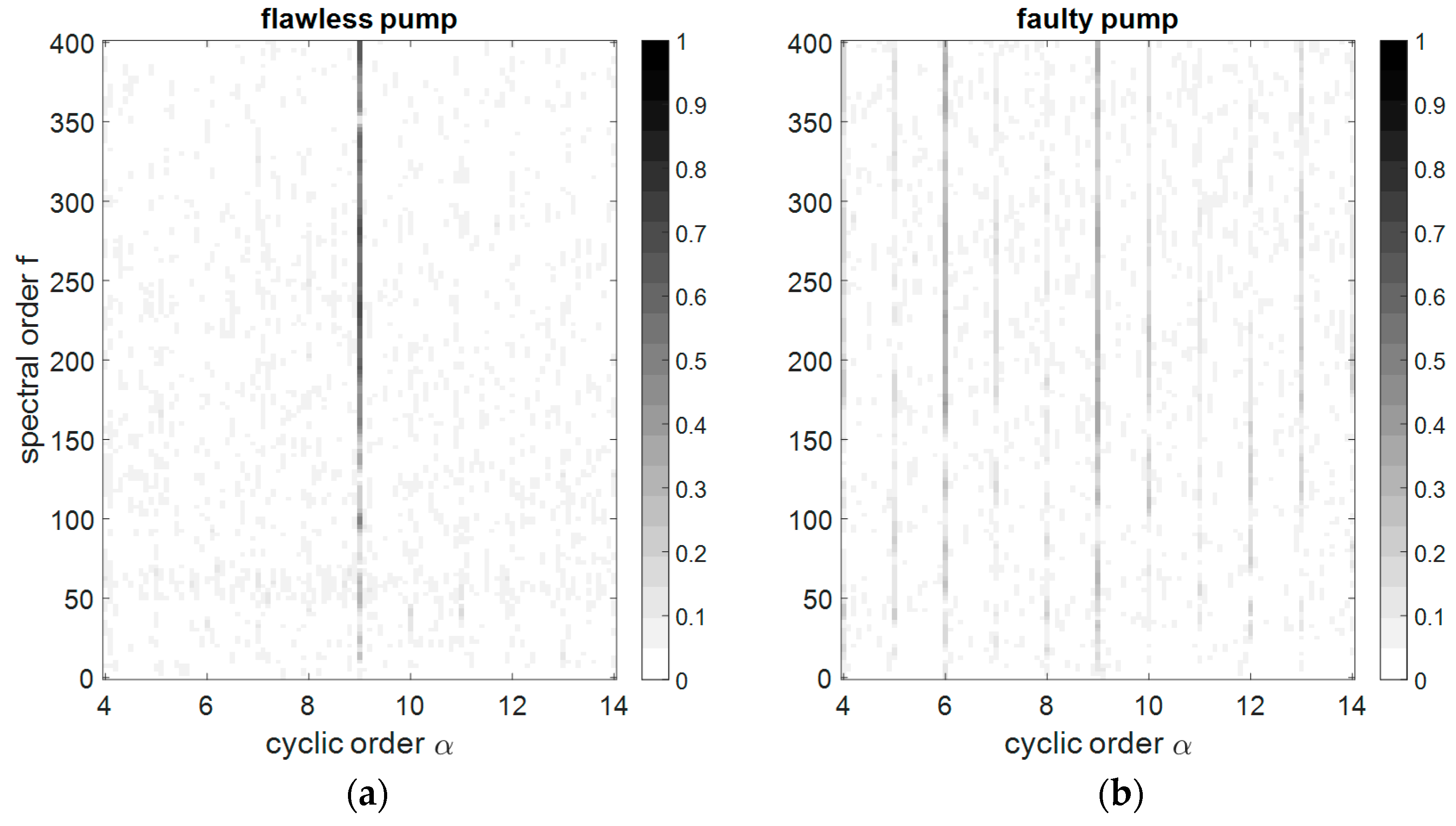
Figure 12 reports the SCD calculated for the signals acquired with sensor 1 with the pump operated at 1500 r/min and 150 bar. The plots show the cyclic order on the x-axis and the spectral order on the y-axis. For the flawless pump (standard), clear modulation at order 9 is present; the power of the random part of the acceleration signal is clearly modulated at the piston’s frequency. For the faulty pump, modulations at other orders, multiples of order 1, are present. In case of worn slippers, not only the periodic part, but also the power modulation of the random part loses the dominant component at order 9 and shows components at multiples of the shaft frequency. The explanation of these phenomena is the differential wear of the slippers; each of them excites the pump vibration in a different manner and the component at order 9 reduces.
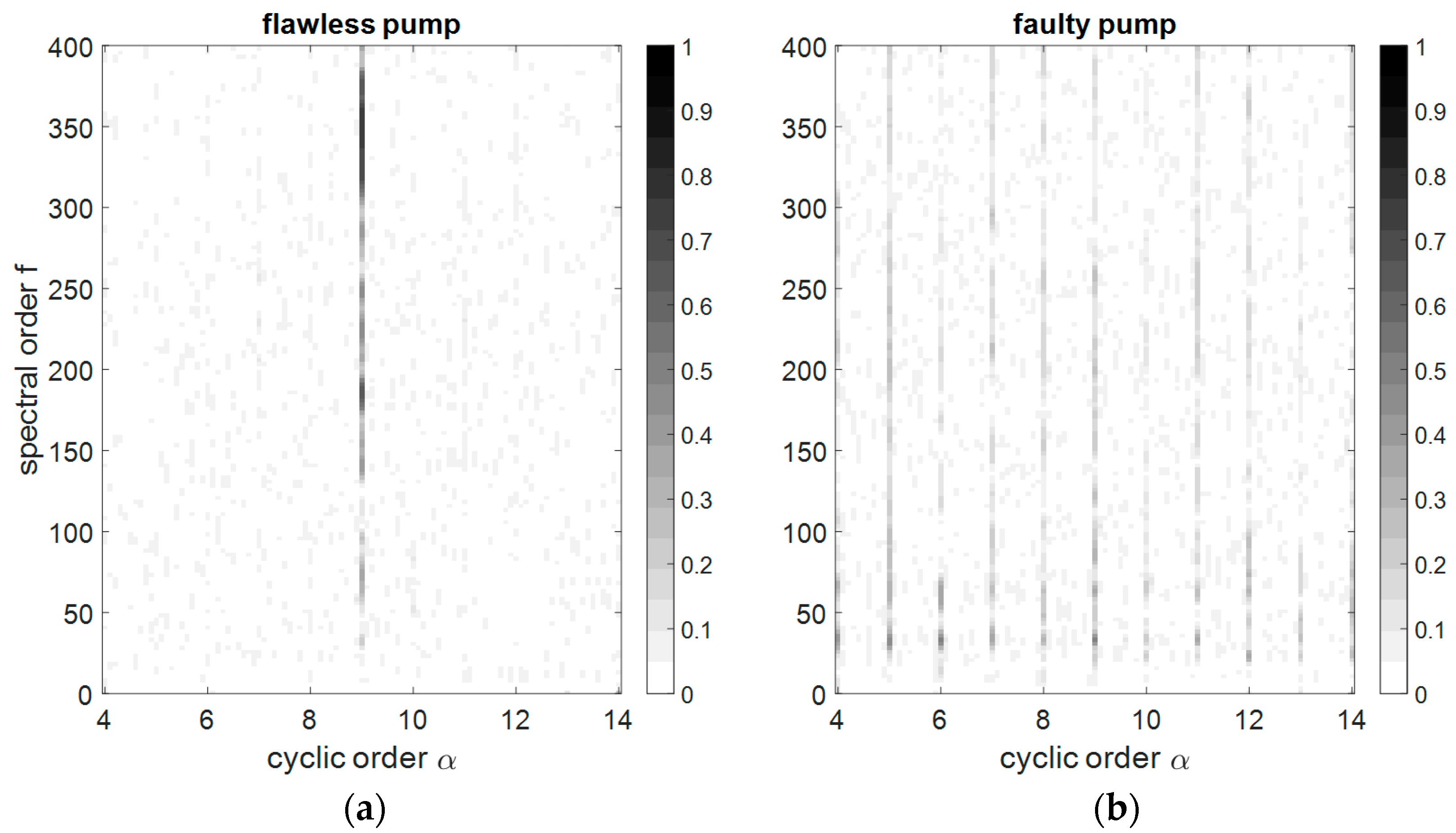
Figure 13 reports the CSC for the same signals considered in Figure 12. For the flawless pump, a clear line at order 9 can be noticed, and this signal shows a clear CS2 behavior at the piston frequency. In the case of the faulty pump, the degree of second-order cyclostationarity at order 9 is lower and comparable to the degree found at multiples of order 1.
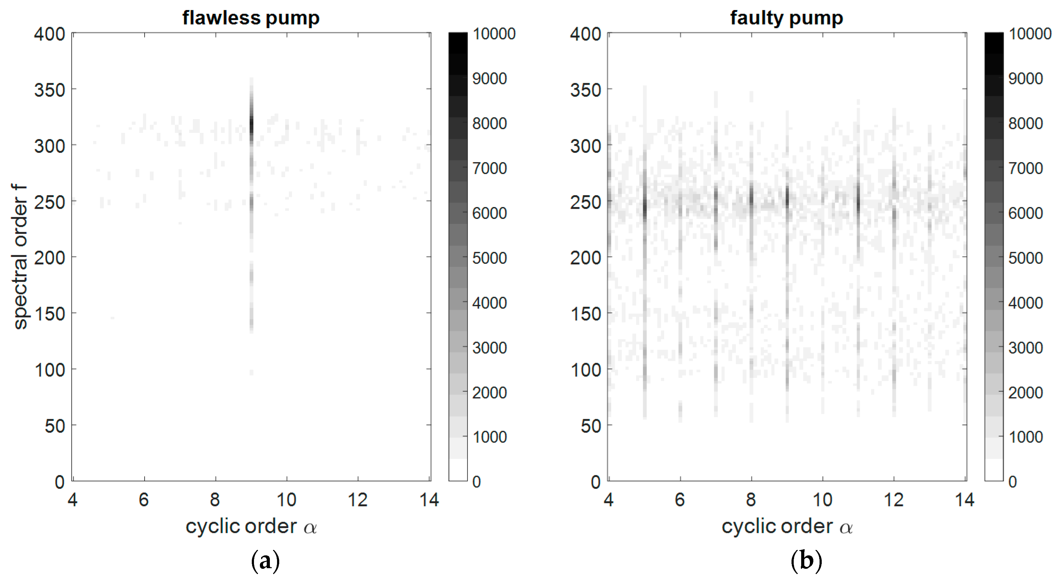
Figure 14 reports the spectral correlation density calculated for the signals acquired with sensor 2 with the pump operated at 1500 r/min and 150 bar; also, in this case, the faulty pump presents power modulations at multiples of order 1 at spectral frequencies around order 250.
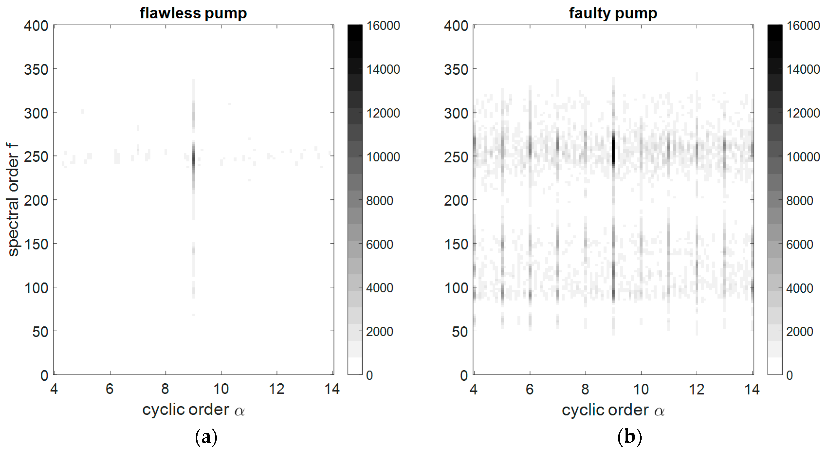
Figure 15 reports the spectral coherence of the signals considered in Figure 14. Figure 16 and Figure 17 reports the SCD and the CSC for the signals acquired with sensor 2 with the pump operated at 2000 r/min and 250 bar. The trends found in the tests performed at 1500 r/min 150 bar, presented in Figure 14 and Figure 15, are confirmed.
Analogue considerations can be extended to the other test conditions not reported for the sake of brevity.
4.4. Assessment
The machine vibrations are the result of the contributions of different sources; an effective signal analysis requires the separation of these contributions in order to avoid interference.
The acceleration signals were acquired by means of two accelerometers installed on the pump case in different positions; since both accelerometers gave the same results, for online diagnostics, only one will be used in order to limit costs and installation space.
The fault related to the worn slippers reduces the excitation at the piston frequency (order 9); this behavior is evident in the CS1 component and in the power modulation of the CS2 components.
The fault considered in this paper could be detected through the first-order cyclostationary analysis, but other common faults, such as cavitation erosion on the port plate and bearing faults, do not affect heavily the periodic part, but induce a change in the CS2 components at specific cyclic frequencies and spectral frequencies.
In this activity, the angular sampling was implemented by using a relative encoder, which is expensive and unsuitable for onboard diagnostics. To solve this drawback, a methodology based on the time sampling of the acceleration signals and a tacho signal for the angular resampling will be studied. Another aspect limiting the application of the proposed approach for online applications is the high computational effort required for the second-order cyclostationary analysis. To address this point, the application of this methodology to a narrow spectral order range will be considered.
5. Conclusions
In this paper, a methodology based on the theory of cyclostationarity is proposed for the analysis of acceleration signals issued by roto-dynamic machines.
The proposed methodology involves the extraction of the periodic component (CS1) by computing the SA of the signal. The calculation of the SA requires an angular sampling performed with a relative encoder, used as a trigger for the acquisitions. The CS1 component was analyzed by computing the FFT. The residual signal, obtained by subtracting the SA from the raw signal, contains only CS2 or higher-order cyclostationary components. In this paper, only the analysis of the CS2 components was addressed because these components are the most significant in roto-dynamic machines. The SCD and CSC were proposed to analyze the CS2 components in the frequency–frequency domain. The methodology was applied to a variable displacement axial-piston pump, and a common fault related to artificially worn slippers was considered. The worn piston slippers condition was detectable through the first-order cyclostationary analysis and was also evident in the second-order cyclostationary analysis of the residual signal. The identification of the fault related to the worn slippers is an important result since this fault is one of the most common for pumps of the swash-plate type.
In future works, the methodology will be tested on a wider set of faults in order to demonstrate that it can be effectively applied for the detection of the most common incipient faults in axial-piston pumps. For online applications, the features of interest can be calculated only, reducing the computational effort and avoiding the calculation of useless parameters.
Author Contributions
P.C. and F.C. conceived and designed the experiments; A.B. and M.P. performed the experiments, analyzed the data and applied the proposed methodology. All the authors wrote the paper.
Funding
This research received no external funding.
Acknowledgments
The authors would like to acknowledge the active support of this research by Casappa S.p.A., Parma, Italy.
Conflicts of Interest
The authors declare no conflict of interest.
Abbreviations
| BCS | Blind Component Separation |
| BSE | Blind Signal Extraction |
| BSS | Blind Source Separation |
| CS1 | First-Order Cyclostationary |
| CS2 | Second-Order Cyclostationary |
| CSC | Cyclic Spectral Coherence |
| FDI | Fault Detection and Identification |
| FFT | Fast Fourier Transform |
| PHM | Prognostics and Health Management |
| PSD | Power Spectral Density |
| RUL | Remaining Useful Life |
| SA | Synchronous Average |
| SCD | Spectral Correlation Density |
References
- Ma, Z.; Wang, S.; Shi, J.; Li, T.; Wang, X. Fault diagnosis of an intelligent hydraulic pump based on a nonlinear unknown input observer. Chin. J. Aeronaut. 2018, 31, 385–394. [Google Scholar] [CrossRef]
- Lu, C.; Wang, S.; Wang, X. A multi-source information fusion fault diagnosis for aviation hydraulic pump based on the new evidence similarity distance. Aerosp. Sci. Technol. 2017, 71, 392–401. [Google Scholar] [CrossRef]
- Tidriri, K.; Chatti, N.; Verron, S.; Tiplica, T. Bridging data-driven and model-based approaches for process fault diagnosis and health monitoring: A review of researches and future challenges. Annu. Rev. Control 2016, 42, 63–81. [Google Scholar] [CrossRef] [Green Version]
- Antoni, J.; Danière, J.; Guillet, F. Effective vibration analysis of IC engines using cyclostationarity. Part I: A methodology for condition monitoring. J. Sound Vib. 2002, 257, 815–837. [Google Scholar] [CrossRef]
- Antoni, J.; Danière, J.; Guillet, F.; Randall, R.B. Effective vibration analysis of IC engines using cyclostationarity. Part II: new results on the reconstruction of the cylinder pressure. J. Sound Vib. 2002, 257, 839–856. [Google Scholar] [CrossRef]
- Yu, J. Machine health prognostics using the Bayesian-inference-based probabilistic indication and high-order particle filtering framework. J. Sound Vib. 2015, 358, 97–110. [Google Scholar] [CrossRef]
- Fan, Z.; Li, H. A hybrid approach for fault diagnosis of planetary bearings using an internal vibration sensor. Measurement 2015, 64, 71–80. [Google Scholar] [CrossRef]
- Cernetic, J. The use of noise and vibration signals for detecting cavitation in kinetic pumps. Proc. Inst. Mech. Eng. Part C J. Mech. Eng. Sci. 2009, 223, 1645–1655. [Google Scholar] [CrossRef]
- Buono, D.; Siano, D.; Frosina, E.; Senatore, A. Gerotor pump cavitation monitoring and fault diagnosis using vibration analysis through the employment of auto-regressive-moving-average technique. Simul. Model. Pract. Theory 2017, 71, 61–82. [Google Scholar] [CrossRef]
- Neill, G.D.; Reuben, R.L.; Sandford, P.M.; Brown, E.R.; Steel, J.A. Detection of incipient cavitation in pumps using acoustic emission. Proc. Inst. Mech. Eng. Part E J. Process Mech. Eng. 1997, 211, 267–277. [Google Scholar] [CrossRef]
- Alfayez, L.; Mba, D. Detection of incipient cavitation and determination of the best efficiency point for centrifugal pumps using acoustic emission. Proc. Inst. Mech. Eng. Part E J. Process Mech. Eng. 2005, 219, 327–344. [Google Scholar] [CrossRef]
- Du, W.; Yang, C.; Li, A.; Wang, L. Wavelet leaders based vibration signals multifractal features of plunger pump in truck crane. Adv. Mech. 2013. [Google Scholar] [CrossRef]
- Wang, J.; Hu, H. Vibration-based fault diagnosis of pump using fuzzy technique. Measurement 2006, 39, 176–185. [Google Scholar] [CrossRef]
- Hodkiewicz, M.R.; Norton, M.P. The effect of change in flow rate on the vibration of double-suction centrifugal pumps. Proc. Inst. Mech. Eng. Part E J. Process Mech. Eng. 2002, 216, 47–58. [Google Scholar] [CrossRef]
- Sinha, J.K.; Rao, A.R. Vibration Based Diagnosis of a Centrifugal Pump. Struct. Health Monit. 2006, 5, 325–332. [Google Scholar] [CrossRef]
- Sakthivel, N.R.; Sugumaran, V.; Babudevasenapati, S. Vibration based fault diagnosis of monoblock centrifugal pump using decision tree. Expert Syst. Appl. 2010, 37, 4040–4049. [Google Scholar] [CrossRef]
- Ramdén, T. Condition Monitoring and Fault Diagnosis of Fluid Power Systems: Approaches with Neural Networks and Parameter Identification; Linköping University: Linköping, Sweden, 1998. [Google Scholar]
- Ramdén, T.; Krus, P.; Palmberg, J.-O. Fault diagnosis of complex fluid power systems using neural networks. In Proceedings of the Fourth Scandinavian International Conference on Fluid Power, Tampere, Finland, 26–29 September 1995; pp. 706–718. [Google Scholar]
- Ramdén, T.; Krus, P.; Palmberg, J.-O. Reliability and sensitivity analysis of a condition monitoring technique. Proc. JFPS Int. Symp. Fluid Power 1996, 567–572. Available online: https://www.jstage.jst.go.jp/article/isfp1989/1996/3/1996_3_567/_article (accessed on 16 July 2018).
- Gao, Y.; Zhang, Q. A Wavelet Packet and Residual Analysis Based Method for Hydraulic Pump Health Diagnosis. Proc. Inst. Mech. Eng. Part D J. Automob. Eng. 2006, 220, 735–745. [Google Scholar] [CrossRef]
- Gao, Y.; Zhang, Q.; Kong, X. Wavelet-based pressure analysis for hydraulic pump health diagnosis. Trans. ASAE 2003, 46, 969–976. [Google Scholar]
- Lu, C.; Wang, S.; Zhang, C. Fault diagnosis of hydraulic piston pumps based on a two-step EMD method and fuzzy C-means clustering. Proc. Inst. Mech. Eng. Part C J. Mech. Eng. Sci. 2016, 230, 2913–2928. [Google Scholar] [CrossRef]
- Du, J.; Wang, S.; Zhang, H. Layered clustering multi-fault diagnosis for hydraulic piston pump. Mech. Syst. Sig. Process. 2013, 36, 487–504. [Google Scholar] [CrossRef]
- Dalla Lana, E.; De Negri, V. A New Evaluation Method for Hydraulic Gear Pump Efficiency through Temperature Measurements. 2006. Available online: https://www.sae.org/publications/technical-papers/content/2006-01-3503/ (accessed on 16 July 2018).
- Casoli, P.; Campanini, F.; Bedotti, A.; Pastori, M.; Lettini, A. Overall efficiency evaluation of a hydraulic pump with external drainage through temperature measurements. ASME. J. Dyn. Syst. Meas. Control 2018, 140, DS-17-1191. [Google Scholar] [CrossRef]
- Antoni, J.; Randall, R.B. Differential diagnosis of gear and bearing faults. ASME. J. Vib. Acoust. 2002, 124, 165–171. [Google Scholar] [CrossRef]
- Antoni, J. Cyclostationarity by examples. Mech. Syst. Signal Process. 2009, 23, 987–1036. [Google Scholar] [CrossRef]
- Antoni, J. Blind separation of vibration components: principles and demonstrations. Mech. Syst. Signal Process. 2005, 19, 1166–1180. [Google Scholar] [CrossRef]
- Elia, G.D.; Cocconcelli, M.; Mucchi, E.; Dalpiaz, G. Combining blind separation and cyclostationary techniques for monitoring distributed wear in gearbox rolling bearings. Proc. Inst. Mech. Eng. Part C J. Mech. Eng. Sci. 2017, 231, 1113–1128. [Google Scholar] [CrossRef]
- Antoni, J.; Bonnardot, F.; Raad, A.; El Badaoui, M. Cyclostationary modelling of rotating machine vibration signals. Mech. Syst. Sig. Process. 2004, 18, 1285–1314. [Google Scholar] [CrossRef]
- Capdessus, C.; Sidahmed, M.; Lacoume, J.L. Cyclostationary processes: Application in gear faults early diagnosis. Mech. Syst. Signal Process. 2000, 14, 371–385. [Google Scholar] [CrossRef]
- McFadden, P.D.; Toozhy, M.M. Application of synchronous averaging to vibration monitoring of rolling element bearings. Mech. Syst. Signal Process. 2000, 14, 891–906. [Google Scholar] [CrossRef]
- Fyfe, K.R.; Munk, E.D.S. Analysis of computed order tracking. Mech. Syst. Signal Process. 1997, 11, 187–205. [Google Scholar] [CrossRef]
- Bonnardot, F.; Randall, R.B.; Antoni, J.; Guillet, F. Enhanced Unsupervised Noise Cancellation (E-SANC) Using Angular Resampling—Application for Planetary Bearing Fault Diagnosis. 2004. Available online: http://perso.univ-lemans.fr/~jhthomas/25_bonnardot.pdf (accessed on 16 July 2018).
Figure 1.
Block diagram of the proposed approach for the analysis of acceleration signals.

Figure 2.
(a) Hydraulic scheme of the experimental layout; (b) Position of the two accelerometers on the pump.
Figure 2.
(a) Hydraulic scheme of the experimental layout; (b) Position of the two accelerometers on the pump.

Figure 3.
(a) Raw signal, (b) synchronous average, and (c) residual signal for the signal acquired with sensor 1 in the case of the flawless pump (1500 r/min, 150 bar).
Figure 3.
(a) Raw signal, (b) synchronous average, and (c) residual signal for the signal acquired with sensor 1 in the case of the flawless pump (1500 r/min, 150 bar).

Figure 4.
(a) Raw signal, (b) synchronous average, and (c) residual signal for the signal acquired with sensor 1 in the case of the faulty pump (1500 r/min, 150 bar).
Figure 4.
(a) Raw signal, (b) synchronous average, and (c) residual signal for the signal acquired with sensor 1 in the case of the faulty pump (1500 r/min, 150 bar).

Figure 5.
Synchronous average for the flawless pump (a) and faulty pump (b) for the signal acquired with sensor 1 (1500 r/min, 150 bar).
Figure 5.
Synchronous average for the flawless pump (a) and faulty pump (b) for the signal acquired with sensor 1 (1500 r/min, 150 bar).

Figure 6.
(a) Raw signal, (b) synchronous average, and (c) residual signal for the signal acquired with sensor 2 in the case of the flawless pump (1500 r/min and 150 bar).
Figure 6.
(a) Raw signal, (b) synchronous average, and (c) residual signal for the signal acquired with sensor 2 in the case of the flawless pump (1500 r/min and 150 bar).

Figure 7.
Synchronous average for (a) the flawless pump and (b) faulty pump for the signal acquired with sensor 2 (1500 r/min, 150 bar).
Figure 7.
Synchronous average for (a) the flawless pump and (b) faulty pump for the signal acquired with sensor 2 (1500 r/min, 150 bar).

Figure 8.
FFT of (a) acceleration signal, (b) synchronous average, and (c) residual signal for the signal acquired with sensor 1 in the case of the flawless pump (1500 r/min, 150 bar).
Figure 8.
FFT of (a) acceleration signal, (b) synchronous average, and (c) residual signal for the signal acquired with sensor 1 in the case of the flawless pump (1500 r/min, 150 bar).

Figure 9.
FFT of the synchronous average for (a) the flawless pump and (b) faulty pump for the signal acquired with sensor 1 (1500 r/min, 150 bar).
Figure 9.
FFT of the synchronous average for (a) the flawless pump and (b) faulty pump for the signal acquired with sensor 1 (1500 r/min, 150 bar).

Figure 10.
FFT of the residual signal for (a) the flawless pump and (b) faulty pump for the signal acquired with sensor 1 (1500 r/min, 150 bar).
Figure 10.
FFT of the residual signal for (a) the flawless pump and (b) faulty pump for the signal acquired with sensor 1 (1500 r/min, 150 bar).

Figure 11.
FFT of the synchronous average for (a) the flawless pump and (b) faulty pump for the signal acquired with sensor 2 (1500 r/min, 150 bar).
Figure 11.
FFT of the synchronous average for (a) the flawless pump and (b) faulty pump for the signal acquired with sensor 2 (1500 r/min, 150 bar).

Figure 12.
SCD around the cyclic order 9 for the signals acquired with sensor 1 at 1500 r/min and 150 bar (∆α = 0.1, ∆f = 2.5). (a) flawless pump; (b) faulty pump.
Figure 12.
SCD around the cyclic order 9 for the signals acquired with sensor 1 at 1500 r/min and 150 bar (∆α = 0.1, ∆f = 2.5). (a) flawless pump; (b) faulty pump.

Figure 13.
CSC around the cyclic order 9 for the signals acquired with sensor 1 at 1500 r/min and 150 bar (∆α = 0.1, ∆f = 2.5). (a) flawless pump; (b) faulty pump.
Figure 13.
CSC around the cyclic order 9 for the signals acquired with sensor 1 at 1500 r/min and 150 bar (∆α = 0.1, ∆f = 2.5). (a) flawless pump; (b) faulty pump.

Figure 14.
SCD around the cyclic order 9 for the signals acquired with sensor 2 at 1500 r/min and 150 bar (∆α = 0.1, ∆f = 2.5). (a) flawless pump; (b) faulty pump.
Figure 14.
SCD around the cyclic order 9 for the signals acquired with sensor 2 at 1500 r/min and 150 bar (∆α = 0.1, ∆f = 2.5). (a) flawless pump; (b) faulty pump.

Figure 15.
CSC around the cyclic order 9 for the signals acquired with sensor 2 at 1500 r/min and 150 bar (∆α = 0.1, ∆f = 2.5). (a) flawless pump; (b) faulty pump.
Figure 15.
CSC around the cyclic order 9 for the signals acquired with sensor 2 at 1500 r/min and 150 bar (∆α = 0.1, ∆f = 2.5). (a) flawless pump; (b) faulty pump.

Figure 16.
SCD around the cyclic order 9 for the signals acquired with sensor 2 at 2000 r/min and 250 bar (∆α = 0.1, ∆f = 2.5). (a) flawless pump; (b) faulty pump.
Figure 16.
SCD around the cyclic order 9 for the signals acquired with sensor 2 at 2000 r/min and 250 bar (∆α = 0.1, ∆f = 2.5). (a) flawless pump; (b) faulty pump.

Figure 17.
CSC around the cyclic order 9 for the signals acquired with sensor 2 at 2000 r/min and 250 bar (∆α = 0.1, ∆f = 2.5). (a) flawless pump; (b) faulty pump.
Figure 17.
CSC around the cyclic order 9 for the signals acquired with sensor 2 at 2000 r/min and 250 bar (∆α = 0.1, ∆f = 2.5). (a) flawless pump; (b) faulty pump.


Table 1.
Operating conditions considered for the acceleration measurements in healthy and faulty conditions.
Table 1.
Operating conditions considered for the acceleration measurements in healthy and faulty conditions.
| Angular Velocity | Swash Angle | Delivery Pressure | |
|---|---|---|---|
| 1500 r/min | 12.8 deg | 150 bar | 250 bar |
| 2000 r/min | 12.8 deg | 150 bar | 250 bar |
© 2018 by the authors. Licensee MDPI, Basel, Switzerland. This article is an open access article distributed under the terms and conditions of the Creative Commons Attribution (CC BY) license (http://creativecommons.org/licenses/by/4.0/).
Share and Cite
MDPI and ACS Style
Casoli, P.; Bedotti, A.; Campanini, F.; Pastori, M. A Methodology Based on Cyclostationary Analysis for Fault Detection of Hydraulic Axial Piston Pumps. Energies 2018, 11, 1874. https://doi.org/10.3390/en11071874
AMA Style
Casoli P, Bedotti A, Campanini F, Pastori M. A Methodology Based on Cyclostationary Analysis for Fault Detection of Hydraulic Axial Piston Pumps. Energies. 2018; 11(7):1874. https://doi.org/10.3390/en11071874
Chicago/Turabian StyleCasoli, Paolo, Andrea Bedotti, Federico Campanini, and Mirko Pastori. 2018. "A Methodology Based on Cyclostationary Analysis for Fault Detection of Hydraulic Axial Piston Pumps" Energies 11, no. 7: 1874. https://doi.org/10.3390/en11071874
Note that from the first issue of 2016, this journal uses article numbers instead of page numbers. See further details here.