From the Balancing Reactive Compensator to the Balancing Capacitive Compensator

Electrical Power Engineering Department, Politehnica University of Timișoara, 300006 Timișoara, Romania
*
Author to whom correspondence should be addressed.
Energies 2018, 11(8), 1979; https://doi.org/10.3390/en11081979
Submission received: 26 June 2018
/
Revised: 25 July 2018
/
Accepted: 26 July 2018
/
Published: 30 July 2018
(This article belongs to the Section F: Electrical Engineering)
Abstract
:Nowadays, improving the power quality at the Point of Common Coupling (PCC) between the consumers’ installations and the distribution system operators’ installations depends more and more on the use of specialized equipment, able to intervene in the network to eliminate or diminish the disturbances. The reactive power compensators remain valid solutions for applications in consumer and electricity distribution, in those situations when the criterion regarding the costs of installing and operating the equipment is more important than the ones related to the reaction speed or the control accuracy. This is also the case of the equipment for power factor improvement and load balancing in a three-phase distribution network. The two functions can be achieved simultaneously by using an unbalanced static var compensator, known as an adaptive balancing compensator, achieved by adjusting the equivalent parameters of circuits containing single-phase coils and capacitor banks. The paper presents the mathematical model for the sizing and operation of a balancing reactive compensator for a three-phase four-wire network and then presents some resizing methods to convert it into a balancing capacitive compensator, having the same functions. The mathematical model is then validated by a numerical application, modelling with a specialized software tool, and by experimental laboratory determinations. The paper contains strong arguments to support the idea that a balancing capacitive compensator becomes a very advantageous solution in many industrial applications.
1. Introduction
The Electric Power Distribution Systems face the problems caused by poor power quality, the most important of which being the high reactive power load, the pronounced load unbalance, the unsymmetrical voltages, nonsinusoidal current and voltage waveforms, a high rms value and highly deformed current flowing on the neutral conductor [1,2,3].
The asymmetry of the three-phase voltage set is primarily due to unbalanced loads, so the methods and means used to limit this asymmetry are directed to preventing or limiting the load unbalance. The measures aimed at preventing the effects of the load unbalance include those that achieve their natural balance. Here are two main methods [1,2,3]:
- the balanced repartition of single-phase or two-phase loads on the phases of the three-phase network;
- connection of unbalanced loads to a higher voltage level, which usually corresponds to the solution of increasing the short-circuit power at their terminals. This is the case of industrial consumers of large power (from hundreds of kVA to tens of MVA) in which power is supplied through their own transformers, other than those of other consumers connected in the same bus. Under these conditions, the Voltage Unbalance Factor decreases proportionally to the increase of the short-circuit power at the connection bus.
The most important methods and means for diminishing/eliminating the load’s unbalances of the three-phase networks are:
- using hybrid solutions, containing components from the above categories [32].
RPCs have been developed mostly over the last 30–40 years, starting from Steinmetz’s balancing compensator, developed over 100 years ago [4].
RPCs are built with passive circuit elements of high reactive power (coils and capacitor banks) and can be divided into two categories, as the equivalent parameters of the compensation circuits are fixed or variable. The most common are the RPCs in the second category, known as Static var Compensators (SVCs) [18,19,20,21,22,23,24]. The SVC construction uses high-power electronic components to enable the switching or adjustment of reactive passive circuit elements. These components are found in the Thyristor Controlled Reactor (TCR) and Thyristor Switched Capacitor (TSC) units and can be controlled by automatic control compensation systems [5,6,7,8,9,13,14,15,16]. By enabling reactive power flow control in an Electric Power Distribution System (EPDS), SVCs are widely used in applications for power factor correction, load balancing, voltage control and flicker mitigation [23].
SPCs are pieces of equipment built as applications of the most performing power electronics technology, based on high-power switching elements: Insulated Gate Bipolar Transistor IGBT or Insulated Gate Commutated Thyristor (IGCT) included into the so-called Solid State Devices (SSDs) [30,31,32,33,34,35].
Developed as versions of the Flexible Alternant Current Transmission System (FACTS) that were adapted for EPDSs, SCs or SPCs are also part of the equipment category type CPDs [46,47,48,49,50]. They have been upgraded over the past decades to provide the industrial and commercial, sensible customers with efficient solutions to improve the power quality at the Point of Common Coupling (PCC).
The most common equipment in the category of SPCs are: Distribution Static Synchronous Compensators (D-STATCOMs) [32,43,51], Dynamic Voltage Restorers (DVRs) [32,35,36,45], Unified Power Quality Conditioners (UPQCs) [42,44,47,48] respectively. The main part of this equipment is a VSI [41,49,50].
Each of these pieces of equipment is characterized by specific applications, as follows [49]:
- UPQC—voltage sag and swell correction, voltage symmetrisation, voltage control, flicker mitigation, reactive power compensation, harmonic filtering, load balancing, active and reactive power control [55].
A comparison between SVC and SPC category equipment, using technical criteria, reveals the net superiority of the latter, because: they can perform more functions in order to increase the power quality in the PCC, allow for a more precise control, have a faster response, are more compact, so they occupy smaller spaces and are quieter. In addition, containing fewer passive circuit elements, they produce lower energy losses and therefore have higher energy efficiency.
However, a technical-economic analysis of similar function solutions (power factor correction, load balancing, voltage control, or flicker mitigation) will find that for equipment like SPC the costs are higher with 30–35% than for equipment like SVC [56]. And for many EPDSs applications for which the response speed or the control accuracy of the compensation are not the main requirements, this cost difference is difficult to justify.
This is also the case of the SVC for power factor improvement and load balancing in four-wire distribution networks, which are the topic of this paper.
Starting from the demonstration that any three-phase electric load can be balanced by unbalanced capacitive compensation, the authors of the present paper have the opinion that an SVC built as an Adaptive Balancing Capacitive Compensator (ABCC) based on TSC banks or even on Contactor Switched Capacitor (CSC) banks, can be the optimal solution for many applications, both in consumer installations and electricity distribution operator’s installations [27,29].
This paper presents the mathematical model for the sizing and operating of a Balancing Reactive Compensator (BRC) for a three-phase four-wire network and then presents a few resizing methods to convert it into a Balancing Capacitive Compensator (BCC).
The correctness of the mathematical model is confirmed in three ways: first through a numerical application performed in Mathcad and by a Matlab-Simulink modelling respectively, both performed under simplifying conditions of the mathematical model and then by experimental laboratory determinations carried out in real electrical circuits.
The work contributes to enforcing the idea that BCC becomes a more advantageous solution both by lowering costs due to the removal of high-power coils and by simplifying the automatic compensation control, for which only TSC banks are used.
2. The “Classic” Method of Sizing a Balancing Reactive Compensator
The application of the symmetric component method to a three-phase four-wire network that feeds a certain load shows that it determines some currents’ flow on the phases that can be decomposed into three symmetric three-phase sets: positive, negative and zero sequence.
Reactive power flow on the positive sequence leads to an increase in the technological energy consumption and thus to the reduction of the efficiency of the distribution network. In addition, it increases the voltage losses on lines and transformers and thus increases the difficulties in the process of voltage control in the network.
The presence of negative and zero sequence currents leads to a series of negative effects on the network and, in those cases where they will lead to the occurrence of negative and zero sequence voltages, they will lead to multiple negative effects on the receivers. The negative and zero sequence currents decrease the efficiency of the distribution and damage the quality of the power supplied to consumers [1,2,3].
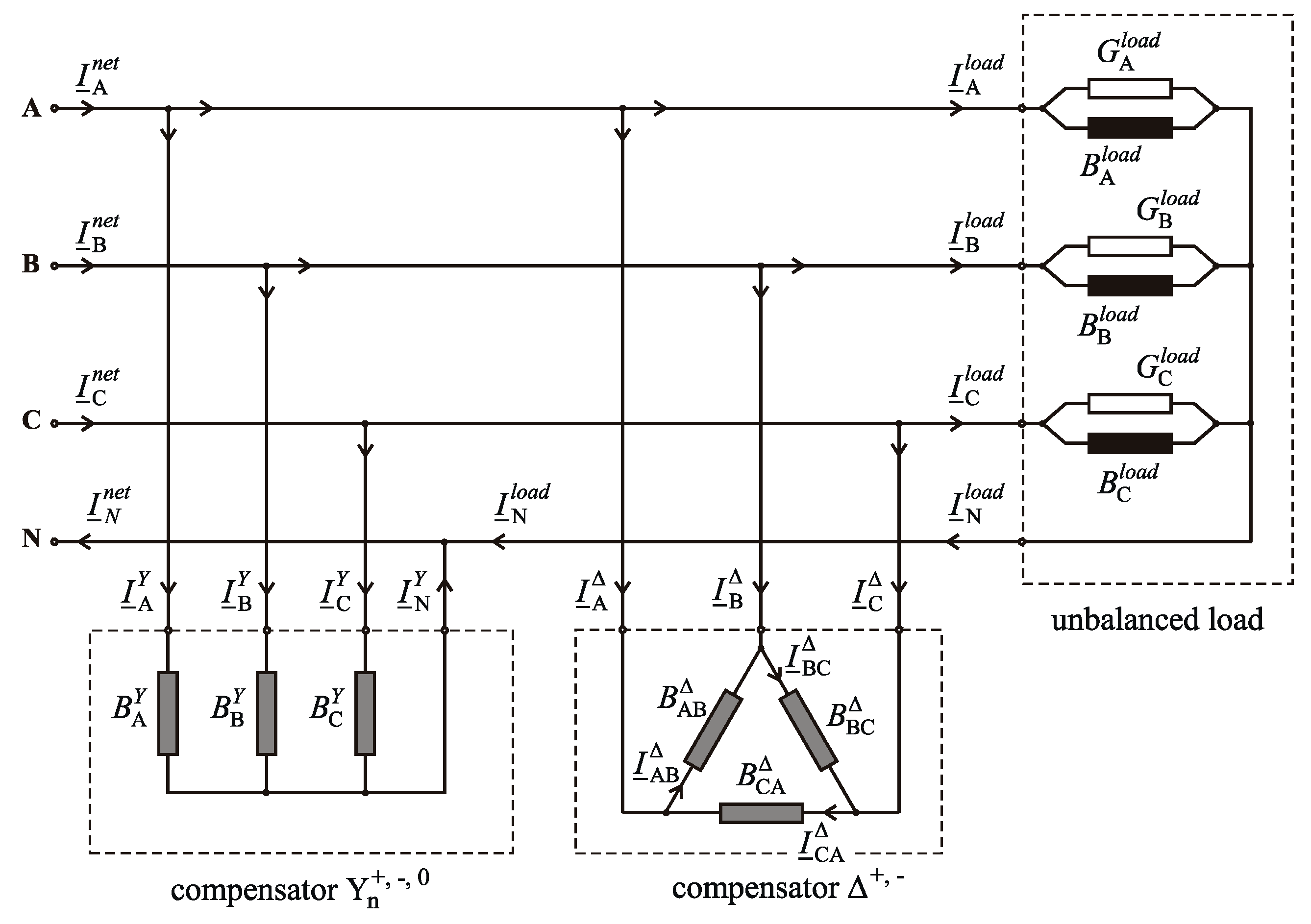
A BRC containing only circuit reactive elements (coils and capacitors) can remove both the reactive components of the positive sequence currents and the negative and zero sequence components of the currents caused by the unbalanced loads. This compensator consists of a three-phase circuit with Yn connection, the only one able to compensate the zero sequence components, and a three-phase circuit with Δ connection respectively, the only one that can compensate the negative sequences currents of the load [9,28] (Figure 1). Obviously, both compensators can compensate the reactive components of the load positive sequence currents. In some papers, the solution is commonly referred to as the generalized Steinmetz compensator [28].
As a result of the Adaptive Balancing Compensator (ABC) action, the load-compensator assembly is seen from the network as a perfectly balanced equivalent load, which consumes only active power [16,26,28]. For the sizing of the six susceptances of the compensator, the analytical expressions are determined applying the conditions of simultaneous cancellation of the symmetrical current components with negative effects on the phases of the load-compensator assembly: the imaginary (reactive) component of the positive sequence current, the real and imaginary components of the negative and zero sequence current components [9]:
Determination of the sequence components of the currents, on the phases of the load—Yn compensator—Δ compensator assembly seen from the network, is done based on the phase components of the currents [28]:
From the above relations we can see that the three-phase voltage set was also considered perfectly symmetrical and in the complex plane , where U is the phase to neutral rms. All susceptances were also considered positive (inductive).
From the relations (8) and (9) some important properties of the compensator can already be inferred [28]:
- because they contain only susceptances, both the Yn compensator and the Δ compensator do not intervene on the flowing of the real (active) components of the positive sequence currents (8.1), (9.1);
- the Δ compensator does not intervene on the flowing of the zero sequence components of the network currents (in fact this is a confirmation of a known property).
Thus, relations (1) turn into [28]:
The unknowns of the problem are the currents on the Yn and Δ compensators’ branches respectively. They have a reactive character, with positive or negative values as the susceptances are inductive or capacitive. First, the expressions of the currents through the six susceptances of the compensator are determined by solving the equation system (1) [9,28]. But to get out of the indetermination, it must be completed by a sixth equation linking the unknowns, independent of the other five. This will be determined based on an additional condition applied to the operation of the compensator. Such a condition, useful to simplifying the solution of the equation system, is [12,28]:
This additional condition will have the effect of Δ compensator intervention only on the negative sequence currents flow. [12,28]. From relations (10.2) and (12) it results:
afterwards, taking into account the relation (9.1), it is obtained:
Analytical solving of the equation system formed by Equations (1) and (11) leads to the solutions [28]:
The expressions for sizing the susceptances in the compensator structure immediately result, written according to the equivalent conductances and susceptances of the load [28]:
The susceptances of the compensator can also be expressed depending on the active and reactive components of the currents or the active and reactive powers on the load phases.
The values of the six susceptances of the compensator result negative or positive, depending on the nature and the level of the load unbalance. For the Δ compensator, one can notice that the algebraic sum of the values of the three susceptances is null, which comes as a consequence of using condition no. (8). This causes that in the structure of this compensator be included at least one inductive susceptance (coil) and at least one capacitive susceptance (capacitor bank).
3. Compensation Mechanism Expressed Based on the Currents Flow
The analytical determination of the currents’ expressions on the phases of the load-compensator assembly in its various three-phase sections is useful in explaining the compensation mechanism. For this, the expressions for phase currents and then for their symmetrical components, expressed in both cases through the phase components of the load currents, are determined.
Thus, by replacing the expressions (14) in relations (4), the currents are obtained on the phases of the Yn compensator [28]:
and afterwards the sequence components:
For the currents on the phases of Δ compensator, from the expressions (6) result:
and the sequence components will be:
Detailing now the relations (2) using the explicit forms from (8), (18) and (20), we can formulate the compensation mechanism that leads to the maximization of the power factor () and total load balancing, using the currents sequence components. It can be immediately seen that:
In fact, all the equations (1) are satisfied. The following statements can be made [28]:
- The Yn compensator cancels the following components of the load currents:
- the imaginary (reactive) component of the positive sequence currents of the load;
- the real and imaginary components of the zero sequence currents of the load;
- a part of the real and imaginary components of the negative sequence currents of the load;
- The Δ compensator compensates two components of the negative sequence currents: one belonging to the load and the other belonging to the Yn compensator.
The only component of the load current remaining uncompensated is the real (active) component of positive sequence currents, component that is found in the currents taken from the supply network (PCC):
The load-compensator assembly takes from the network identical currents on the phases, which only have an active component, whose rms values are equal to each other and equal to the average of the three rms values of the active currents on the load phases.
4. Compensation Mechanism Expressed Based on the Powers Flow
Knowing the currents’ expressions, the powers expressions can easily be found. For the Yn compensator we obtain:
It is observed that the active powers on the Yn compensator phases are null, which is natural because it contains only susceptances. Regarding the values of the reactive powers on the phases of the Yn compensator, it can be observed that they depend both on the reactive power values of the load and on the active powers. It can also be observed that:
Therefore, the Yn compensator is the one that achieves the total compensation of the reactive power of the load.
Concerning the powers on the Δ compensator phases, it results:
It is interesting to note that both the sizing of the Δ compensator’s susceptances and its intervention on the phase powers flow, depend only on the active loads.
Although it contains only susceptances (coils and capacitors), the Δ compensator intervenes on the active powers flowing on the phases. On some phases the active powers are positive while on others negative, depending on the size and the unbalance of the active load. The resulting values are in fact the differences between the values of the active powers of the load and their average value, which are obtained on each phase as a result of balancing (22). The Δ compensator takes active power from the phases in which it is in excess and delivers it towards the phases where it is deficient. This determines a redistribution of the active powers between the phases, thus balancing them. However, throughout the three phases, the Δ compensator does not change the active powers flowing, because:
The Δ compensator also achieves an unbalanced compensation of reactive powers. On some phases it’s doing an inductive compensation and on others, capacitive, depending on the size and the unbalance level of the active loads. However, throughout the three phases, the Δ compensator does not change the reactive powers flowing, because:
5. Resizing from the Condition of Coils Elimination
The “classical” sizing method presented above is very useful in that it simplifies the mathematical solving and then allows easy understanding of the mechanism of the active and reactive loads’ balancing.
However, the condition that the sum of the susceptances values of the Δ compensator being zero (12), which makes it contain both capacities and inductances, is not a useful sizing criterion from a practical point of view. Firstly, because of the construction of an unbalanced compensator containing coils, it leads to increased costs, including a complex automatic control system needed to be used with variable loads (TCR). Secondly, the fact that the entire capacitive reactive power required to compensate the positive sequence inductive reactive power of the load is allocated to the Yn compensator causes an unreasonable use of the capacitors. It is known that a capacitor connected between phase and neutral (supplied with phase to neutral voltage in Yn connection) supplies to the network a reactive power three times lower than if it was connected between two phases (supplied with phase to phase voltage in Δ connection).
Hence the idea of sizing a compensator type BRC that contains only capacitor banks, which, in addition to eliminating the disadvantages presented above, brings a major advantage. It is about the possibility of using a simple automatic control system type TSC, which allows adaptation to variable loads, by switching single phase capacitor bank steps.
The new sizing methods further proposed start from the “classical” sizing method, as the initial solution to the problem, which is then corrected by applying the principle of the capacitive reactive power transfer from the Yn compensator to the Δ compensator, so that it can obtain only negative or null values for all the susceptances.
Typically, by applying the classical sizing method, the Δ compensator results in one or two inductive susceptances, and the Yn compensator only with capacitive susceptances, due to the fact that it has the task of capacitive compensation of the positive sequence.
Without affecting the compensation mechanism, the excess reactive capacitive power on the positive sequence installed in the Yn compensator is transferred totally or partially to the Δ compensator. The value of the reactive capacitive power on the positive sequence, available for transfer, depends on the average power factor of the load and on the degree and the nature of its unbalance. For low average power factor loads, the capacitive reactive power requirement for compensation is high, which allows a high level of balancing or even total load balancing.
Two cases can be distinguished:
case 1—the capacitive reactive power available for the transfer is of low value, insufficient to achieve total load balancing;
case 2—the capacitive reactive power available for the transfer is of high value, sufficient to obtain the total compensation of the reactive power of the load on the positive sequence and the total load balancing.
Thus, for the resizing the susceptances of the Yn and Δ compensators, there are the following versions:
version 1, case 1—total transfer of capacitive reactive power; some susceptances of the Δ compensator are positive (inductive), so they will be canceled. A partial load balancing is achieved.
version 2, case 2—partial transfer of capacitive reactive power, so that all six susceptances of the compensator become negative (capacitive).
version 3, case 2—partial transfer of capacitive reactive power, up to the level of cancellation the lowest capacitive susceptance of the Yn compensator.
version 4, case 2—partial transfer of capacitive reactive power, up to the level of cancellation of the largest inductive susceptance of the Δ compensator.
The transfer of the reactive power on the positive sequence between the two compensators is done in fact by the symmetrical change, of the susceptances values of one of the compensators, and the symmetrical change, in opposite sense, of the susceptances values of the other compensator. The computing equations used are:
The transfer of capacitive reactive power on the positive sequence from the Yn compensator to the Δ compensator is obtained if and:
In versions 2, 3 and 4, such a transfer will cause the two compensators to keep their functions of compensation on the negative and zero sequence exactly at the same level as the initial sizing. However, the Yn compensator substantially reduces its contribution, even totally to capacitive compensation on the positive sequence, while the Δ compensator takes over this function, which it did not have initially. This correction of the initial sizing leads to a more efficient use of the capacitors.
In addition to the sizing versions obtained from the classical solution of capacitive reactive power transfer on the positive sequence presented above, the present paper also takes into account a method that stems from an observation resulting from the compensation mechanism: Yn compensator is the only one that can intervene on the zero sequence currents flowing. It compensates the zero sequence currents of the load, which leads to the cancellation of the neutral conductor current.
Therefore, a valid sizing criterion is to impose to the Yn compensator the function of cancellation the zero sequence of the load currents, having a structure formed only by negative (capacitive) susceptances. We will further refer to the sizing version resulted by applying this criterion, as version 5, in order to associate it with the four ones previously defined.
In order to obtain the relations for sizing the susceptances of the Yn compensator, the condition set in step 1 is:
from which result the conditions:
By referring to relations (7) and (8), we obtain the equations from which result the unknowns of the problem or :
respectively:
The third condition imposed to exit from the indeterminate equation system (34) is the nullification of the value of one of the susceptances. If the known terms in the Equations (34) are noted:
three solutions of the problem result:
In normal situations of the load structure, one of the three solutions will have two negative susceptances. This will be the solution applied to the construction of the Yn compensator and based on which the method goes to step 2: the Δ compensator sizing.
This operation will be done from the observation that the Yn compensator sized in step 1, completely compensates the zero sequence of the load current. So Yn compensator together with the load forms a three-phase assembly with Yn connection in which the flowing of the zero sequence components has been eliminated. The equivalent admittances of this assembly are:
Due to this property, this assembly can now be converted into an equivalent one, having Δ connection, which is supplied from the three-phase without neutral conductor and having the equivalent admittances:
For a three-phase load having the equivalent scheme with Δ connection, the total compensation of reactive power on the positive sequence and perfect load balancing can be achieved by means of an unbalanced Δ compensator. The values of the susceptances in its structure are obtained by the conditions:
This time the equation system (41) has a unique solution [9,12,15]. The susceptances of the Δ compensator expressed depending on the conductances and on the susceptances of the equivalent load are determined with the relations [28]:
This fifth version of sizing the two circuits of the compensator has great chances of success in leading to negative values for all susceptances, if applied in case 2 regarding the characteristics of the unbalanced load, defined above. In such a situation, version 5 of sizing becomes identical to version 3.
The methods of resizing a BRC in order to transform it into a BCC are a continuation of the mathematical model used for sizing and explaining the mechanism of BRC operation. To comprehend the resizing principle, consisting in the redistribution of the reactive capacitive compensating power on the positive sequence, from the Yn compensator to the Δ compensator, it is necessary to preliminary understand the mathematical model of the BRC. For this purpose, Section 2, Section 3 and Section 4 of this paper summarize familiar elements, previously developed by the same authors [26,27,28]. The new contributions of this paper consist of the mathematical model of the resizing methods (Section 5), respectively the presentation of the results of certain applications for their validation (Section 6).
6. Case Studies
The following are the results of the use of two software tools for the numerical study of the sizing and operation of a BRC installed in a four-wire, low-voltage distribution network.
Out of the sizing versions described above, only two examples are presented below: the “classical” version, interesting by its effects (BRC), and version 5 respectively, considered significant for a capacitor structure formed only by capacitor banks (BCC).
First, the results of the sizing and calculation of the current flow in phase components and in symmetrical (sequence) components, and of the power flow on the load-compensator assembly phases in various of its sections, performed using the Mathcad (version 2017b, Parametric Technology Corporation, Boston, MA) software tool (Table 1, Table 2, Table 3 and Table 4), respectively, are presented).
The calculation was done by considering some usual simplifying conditions:
- the source is considered an ideal one, providing a set of perfectly symmetrical and sinusoidal voltages, so that the unbalance will occur only in currents;
- the circuit elements type R, L, C are considered ideal, perfectly linear;
- the impedances of the connections between the components of the circuit, including the impedance of the neutral conductor, are neglected.
The rms value of the phase to neutral voltage is 230 V, the phasor corresponding to the phase to neutral voltage A is placed in the real axis of the complex plane and the working frequency is 50 Hz.
From the analysis of the results obtained using Mathcad tool, the following can be observed:
- In both sizing versions, the Yn compensator only intervenes on reactive power flow on phases, providing reactive power;
- In the BRC version, the Yn compensator supplies the entire reactive power required to fully compensate the reactive power of the load on the positive sequence, whereas in version 5 this role is predominantly taken by the Δ compensator;
- In the BRC version, the Δ compensator makes a redistribution of the active and reactive powers respectively, between the phases without changing their balance over the three phases; it only intervenes in the negative sequence currents flow;
- The Δ compressor from the BRC structure, although containing only reactive circuit elements (two capacities and one inductance), also intervenes on the phase active power flow;
- In both sizing versions, the Δ compensator intervenes identically on the active power flow, which is the effect of the fact that it intervenes identically on the negative sequence currents flow; the conclusion is natural, since the intervention is different only on the positive sequence currents flow;
- The (Yn +Δ) compensator assembly has exactly the same effect in both sizing versions: it totally compensates the five components of the load sequence currents: the reactive component of the positive sequence currents, the real and imaginary components of the negative and zero sequence components.
It is obvious that the BCC version of the compensator is more advantageous than the classical version BRC because it contains only capacities, so single phase capacitor banks if we talk about a real structure.
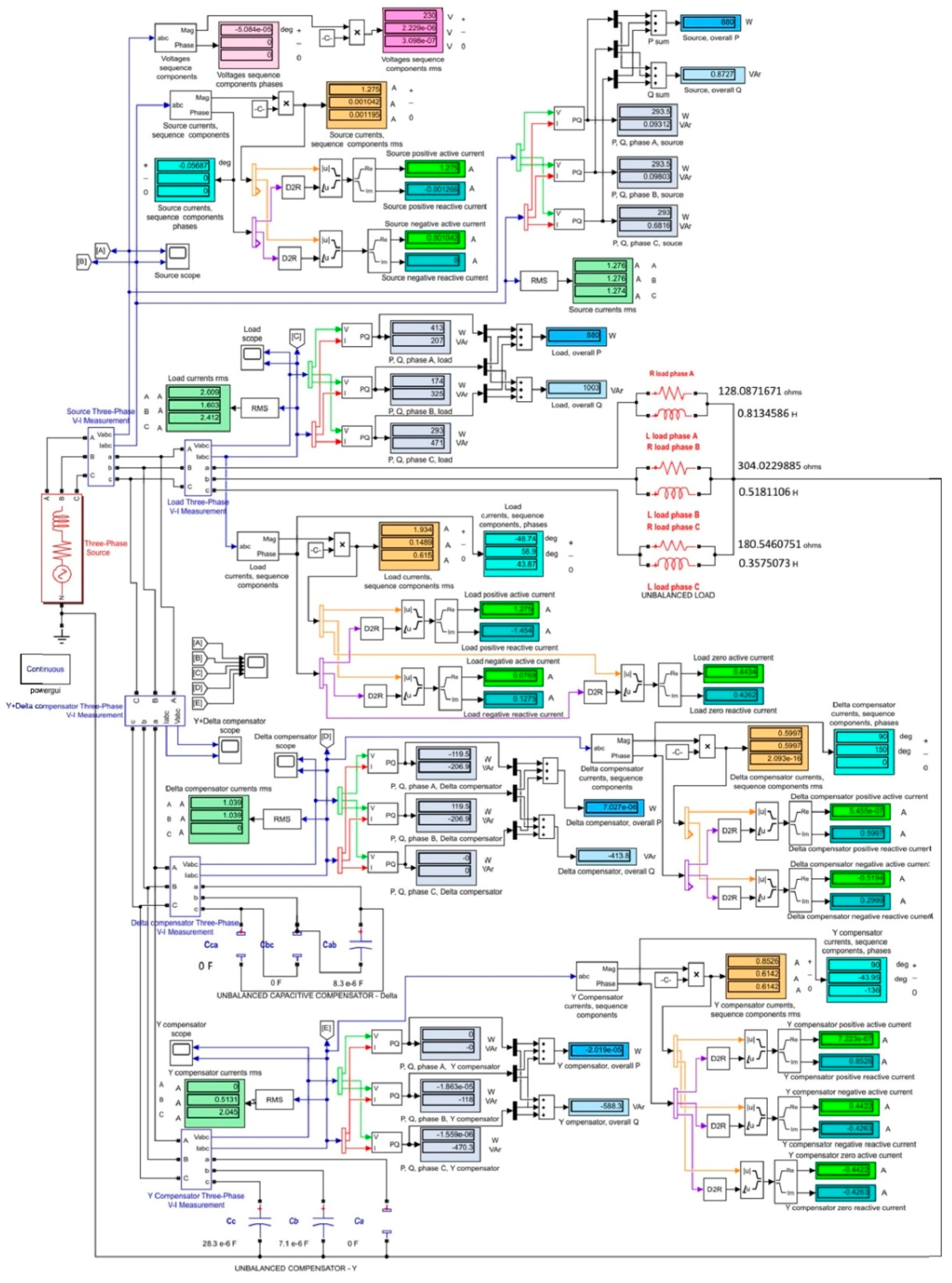
To verify the results obtained using Mathcad, a modelling of the same three-phase circuits was carried out using the Matlab-Simulink tool, SimPowerSys module (see Figure 2).
Only the BCC was considered, sizing version number 5(3). The capacities values of the two compensators were slightly corrected against the values obtained by computation to be reproduced better in the laboratory experiment. It can be observed that for normal operating conditions, the virtual measurement instruments have basically indicated the same power and current values as those obtained by computing in Mathcad.
Figure 3a–e give waveforms obtained with virtual oscilloscopes installed in the four sections considered significant, the terminals of the following elements: load, Yn compensator, Δ compensator, Yn + Δ compensator and network (PCC) respectively.
The effect of the action of the two components of the compensator can be seen in the waveforms of the three currents on the phases of the circuit in the section from the source (PCC), Figure 3e. The perfect balancing, positive sequence, and currents amplitude reduction can be seen as a result of the compensation of reactive components of positive sequence currents. An overlap of these waveforms beyond those of phase to neutral voltages shows zero phase shift between current and voltage on the same phase, proving the active character of currents and powers.
The regime presented is one that has a particular property, that the Yn compensator has an open circuit branch () and the Δ compensator has two open circuit (, ) and nevertheless the balancing obtained is almost perfect.
The calculations and modelling performed in this case study demonstrate that compensation of the inductive reactive power of three-phase unbalanced loads and at the same time the total load balancing, can be obtained by unbalanced capacitive compensation, using a SVC-type ABCC.
7. Experimental Determinations
The correctness of the mathematical model and of the BRC resizing method for the purpose of transforming it into a BCC, by transferring the positive sequence compensation reactive power from the Yn compensator to the Δ compensator, was confirmed by experimental laboratory determinations.
The schema of the built circuit was that shown in Figure 1. Circuit elements have parameter values equal to those applied in the numerical study and Simulink model applied for the study of the BCC, sizing version 5(3), shown above.
So, the values of these parameters were:
- —
- for the three-phase load: , , , , , ;
- —
- for the Yn compensator: , , ;
- —
- for the Δ compensator: , , .
A power quality analyzer, type MAVOWATT 230, was used for measurements.
For the five sections of interest in the three-phase circuit, the following graphs were drawn:
- rms values of voltages and currents by phases, active and reactive powers;
- the waveforms of the phase voltages and corresponding currents;
- phasor diagrams of phase voltages and phase currents.
The values obtained by experimental determinations are presented in Figure 4. The differences between the experimental and the computationally obtained values are mainly due to the fact that under real conditions; the simplifying assumptions used in the calculation and modelling are no longer valid. Experimental determinations were performed under the following practical conditions:
- The power supply used was a three-phase autotransformer connected to the laboratory’s alternating current network with a nominal voltage of 230/400 V. Therefore, both due to the network and because of the constructive asymmetry of the autotransformer, the supply voltages of the experimental circuit make up an unbalanced voltage set, both as rms values and as phase-shifting angles. The percentage deviations of the measured values relative to the reference values (imposed in the determinations by calculation and simulation) are up to 1.13% for the rms values and 0.75% for the phase shifts.
- Asymmetry of the three-phase voltage set causes the negative and zero sequence components occurring. However, their percentages obtained by reference to the positive sequence component do not exceed 2.2%.
- The network and autotransformer are the main causes of voltages waveforms distortion. However, THD for phase voltages does not exceed 1.5%.
- Currents waveforms distortion is also caused by the nonlinearity of circuit elements (ferromagnetic core coils and electrolytic capacitors) to which non-sinusoidal voltages are applied. The currents waveforms are more distorted than the voltages waveforms, but the THD for the currents does not exceed 5%.
- Circuit elements are resistors, ferromagnetic core coils and electrolytic capacitors. They do not intervene in the circuit only by equivalent parameters of type R, L or C, but also by additional equivalent electrical resistances corresponding to the losses of active power in ferromagnetic cores and dielectric materials.
- The measurement system used is a Mavowatt 230 type which is actually a three-phase power quality analyzer. Measurement errors are small enough but depend on the values of the electrical amounts in the circuit to which they are connected. This is especially the case for measuring currents. Since current measurements are made by means of ampermetric clamps with rated currents of 10 A, low rms values are usually measured with increased errors (±5%). Their phase shifts are determined with greater errors. Also distortion of currents and voltages waveforms causes an additional increase in measurement errors.
All these conditions described above lead to deviations from the simplifying conditions considered in the determinations by numerical calculation and simulation. However, as can be seen from the results of the measurements, these deviations are not likely to alter the operation of the modeled circuit.
The main comments regarding the results of the experimental determinations are as follows:
- ▪
- There is no difference between the values obtained by the numerical calculation and those obtained by the simulation. This is natural, given that they have been made under simplified (ideal) conditions. Matlab-Simulink modeling confirms the correctness of the mathematical model which is the basis for the numerical calculation.
- ▪
- The largest percentage deviation is −7.64% and the lowest is −0.2%.
- ▪
- The most visible deviations are those of the values that should be null:
- -
- the negative and zero sequence components of the voltages,
- -
- the active powers on the Yn compensator phases (which contain only capacitors),
- -
- the rms value of the current on the phase A of the Yn compensator (open branch),
- -
- the active and reactive powers on the phase C of the ∆ compensator,
- -
- the sum of the active powers on the ∆ compensator phases,
- -
- the reactive powers on the phases of the load-BCC assembly (in the PCC),
- -
- the negative and zero sequence components of the currents in the PCC.
- ▪
- Although experimental determinations have been influenced by many error sources, deviations of measured values from calculated values can be neglected. These deviations do not disturb the BCC operation. It performs well the two functions for which it has been sized: power factor improvement and load balancing in the PCC.
- ▪
- The measured values confirm the correctness of the mechanism of active and reactive load balancing by unbalanced capacitive compensation, mechanism anticipated by mathematical model development:
- -
- cancellation of the zero sequence currents of the load is accomplished only by the Yn compensator, which supplies a set of zero sequence currents practically equal to their rms value and shifted by 180°;
- -
- the negative sequence current of the load and the reactive component of the positive sequence current of the load are canceled by the contribution of both Yn and Δ compensators; the two compensators perform together the reactive powers compensation and balancing;
- -
- the ∆ compensator, although containing only one single-phase capacitor bank, takes active power from phase A, where it is in excess (over the average value), and delivers it back on phase B where there is an active power deficiency; the ∆ compensator is the one that performs the active powers balancing;
- -
- although it contains only capacitor banks, the compensator achieves, not only the compensation of the reactive power of the load, but also the balancing of the active powers on its phases.
8. Conclusions
Nowadays, despite the proliferation of high power SSD equipment dedicated to intervene in electrical networks to improve the power quality, compensator-type SVCs remain valid solutions for applications in the installations of consumers and operators of electric power networks for whom the cost criterion for the acquisition and operation of these types of equipment is more important than those relating to the reaction speed or the control accuracy.
For a large number of industrial or commercial consumers, a SVC-type ABCC that manages the individual switching of the steps of the single-phase capacitor banks, becomes a very advantageous solution, both by reducing costs due to the removal of high power coils, and by simplifying the automatic compensation control.
The article brings important arguments to support the efficiency of an SVC type ABCC, with the following contributions:
- -
- the detailed mathematical model of a BRC’s operation and the explanation based on it of the mechanism of balancing the active and reactive three-phase loads by unbalanced reactive compensation;
- -
- developing a method of resizing a BRC for the purpose of transforming it into a BCC by transferring the reactive capacitive compensating power to the positive sequence between the two components of the compensator;
- -
- validation of the mathematical model using both numerical and modeling software tools as well as experimental laboratory determinations.
The results of the theoretical and experimental study demonstrate that the total compensation of reactive power on positive sequence and the total balancing of loads in three-phase four-wire networks can be achieved by unbalanced capacitive compensation.
Author Contributions
Conceptualization, Methodology, Validation: A.P.; Investigation: A.P., A.B., F.M.-M.; Writing-Original Draft Preparation: A.P.; Writing-Review & Editing: A.B., F.M.-M.
Funding
This research received no external funding.
Conflicts of Interest
The authors declare no conflict of interest.
Abbreviations and Notations
| PCC | Point of Common Coupling; |
| RPC | Reactive Power Compensator; |
| SVC | Static var Compensator; |
| ABC | Adaptive Balancing Compensator; |
| ABCC | Adaptive Balancing Capacitive Compensator; |
| BRC | Balancing Reactive Compensator; |
| BCC | Balancing Capacitive Compensator; |
| SPC | Switching Power Converter; |
| TCR | Thyristor Controlled Reactor; |
| TSC | Thyristor Switched Capacitor; |
| CSC | Contactor Switched Capacitor |
| EPDS | Electric Power Distribution System; |
| IGBT | Insulated Gate Bipolar Transistor; |
| IGCT | Integrated Gate Commutated Thyristor; |
| SSD | Solid State Device; |
| FACTS | Flexible Alternant Current Transmission System; |
| CPD | Custom Power Device; |
| D-STATCOM | Distribution Static Synchronous Compensator; |
| DVR | Dynamic Voltage Restorer; |
| UPQC | Unified Power Quality Conditioner; |
| VSI | Voltage Source Inverter; |
| , , | phasors of positive, negative and zero sequence components of the phase currents at the network (in PCC); |
| , , | phasors of positive, negative and zero sequence components of the phase currents at the load; |
| , , | phasors of positive, negative and zero sequence components of the phase currents at Yn compensator; |
| , , | phasors of the phase currents at Yn compensator; |
| , , | rms values of the compensation currents at Yn compensator; |
| , , | phasors of positive, negative and zero sequence components of the phase currents at Δ compensator; |
| , , | phasors of the phase currents at Δ compensator; |
| , , | phasors of the currents on Δ compensator branches; |
| , , | rms values of the compensation currents on Δ compensator branches; |
| , , | phasors of phase to neutral voltages; |
| , , , | phasors of the currents on the phase conductors respectively on the neutral conductor at the network (in PCC); |
| , , , | phasors of the currents on the phase conductors respectively on the neutral conductor at the load; |
| , , … | rms values of the active and reactive components of the phase currents at the load; |
| , , | load admittances for Yn equivalent circuit; |
| , , , , , | equivalent conductances and susceptances of the load; |
| , , , , , | equivalent admittances and susceptances of Yn compensator; |
| , , , , , | equivalent admittances and susceptances of Δ compensator; |
| , , , … | apparent, active and reactive powers on the Yn compensator phases; |
| , , , … | apparent, active and reactive powers on the Δ compensator phases; |
| A | Stokvis rotation operator . |
References
- Dugan, R.C.; McGranaghan, M.F.; Beaty, H.W. Electric Power Systems Quality, 2nd ed.; McGraw-Hill Education: New York, NY, USA, 2006; ISBN 978-0071386227. [Google Scholar]
- Antonio, M.M. Power Quality: Mitigation Technologies in a Distributed Environment; Springer: London, UK, 2007; ISBN 978-1-84628-772-5. [Google Scholar]
- Ewald, F.F.; Mohammad, A.S.M. Power Quality in Power Systems and Electrical Machines; Elsevier Academic Press: London, UK, 2008; ISBN 978-0-08-055917-9. [Google Scholar]
- Steinmetz, C.P. Theory and Calculation of Electrical Apparatus; McGraw Hill Book Company: New York, NY, USA, 1917. [Google Scholar]
- Grandpierr, M.; Trannoy, B. A stationary power device to rebalance and compensate reactive power in three-phase network. In Proceedings of the 1977 IAS Annual Conference, Los Angeles, CA, USA, 2–6 October 1977; pp. 127–135. [Google Scholar]
- Klinger, G.C. Kompensation und symmetirung fur Mehrphasensysteme mit beliebigen Spanungdverlauf. ETZ Arch. 1979, H.2, 57–61. [Google Scholar]
- Gyugyi, L.; Otto, R.; Putman, T. Principles and applications of static thyristor-controlled shunt compensators. IEEE Trans. Power Appl. Syst. 1978, PAS-97, 1935–1945. [Google Scholar] [CrossRef]
- Miller, J.E. Reactive Power Control in Electric Systems; John Wiley & Sons: New York, NY, USA, 1982. [Google Scholar]
- Gueth, G.; Enstedt, P.; Rey, A.; Menzies, R.W. Individual phase control of a static compensator for load compensation and voltage balancing. IEEE Power Eng. Rev. 1987, 2, 898–905. [Google Scholar] [CrossRef]
- Czarnecki, L.S. Reactive and unbalanced currents compensation in three-phase asymmetrical circuits under nonsinusoidal conditions. IEEE Trans. Instrum. Meas. 1989, 38, 754–759. [Google Scholar] [CrossRef]
- Czarnecki, L.S. Minimization of unbalanced currents in three-phase asymmetrical circuits with nonsinusoidal voltage. IEE Proc. B Electr. Power Appl. 1992, 139, 347–354. [Google Scholar] [CrossRef]
- Lee, S.Y.; Wu, C.J. On-line reactive power compensation schemes for unbalanced three-phase four wire distribution systems. IEEE Trans. Power Deliv. 1993, 8, 1235–1239. [Google Scholar] [CrossRef]
- Czarnecki, L.S. Supply and loading quality improvement in sinusoidal power systems with unbalanced loads supplied with asymmetrical voltage. Arch. Elektrotech. 1994, 77, 169–177. [Google Scholar] [CrossRef]
- Czarnecki, L.S.; Hsu, S.M. Thyristor controlled susceptances for balancing compensators operated under nonsinusoidal conditions. IEE Proc. Electr. Power Appl. 1994, 141, 177–185. [Google Scholar] [CrossRef]
- Czarnecki, L.S.; Hsu, S.M.; Chen, G. Adaptive balancing compensator. IEEE Trans. Power Deliv. 1995, 10, 1663–1669. [Google Scholar] [CrossRef]
- Oriega de Oliveira, L.C.; Barros Neto, M.C.; de Souza, J.B. Load compensation in four-wire electrical power systems. In Proceedings of the International Conference on Power System Technology, Perth, WA, Australia, 4–7 December 2000; pp. 1575–1580. [Google Scholar]
- Arendse, C.; Atkinson-Hope, G. Design of a Steinmetz Symmetrizer and application in unbalanced network. In Proceedings of the 45th International Universities Power Engineering Conference UPEC2010, Cardiff, UK, 31 August–3 September 2010; pp. 1–6. [Google Scholar]
- Lee, S.-Y.; Wu, C.-J.; Chang, W.-N. A compact control algorithm for reactive power compensation and load balancing with static VAr compensator. Electr. Power Syst. Res. 2001, 58, 63–70. [Google Scholar] [CrossRef]
- Mayordomo, J.G.; Izzeddine, M.; Asensi, R. Load and voltage balancing in harmonic power flows by means of static var compensators. IEEE Trans. Power Deliv. 2002, 17, 761–769. [Google Scholar] [CrossRef]
- Grünbaum, L.; Petersson, A.; Thorvaldsson, B. FACTS improving the performance of electrical grids. In ABB Review (Special Report on Power Technologies); ABB Group: Zürich, Switzerland, 2003; pp. 13–18. [Google Scholar]
- Dixon, J.; Morán, L.; Rodríguez, J.; Domke, R. Reactive power compensation technologies, state of-the-art review. Proc. IEEE 2005, 93, 2144–2164. [Google Scholar] [CrossRef]
- Quintela, F.R.; Arevalo, J.M.G.; Redondo, R.C. Power analysis of static VAr compensators. Int. J. Electr. Power Energy Syst. 2008, 30, 376–382. [Google Scholar] [CrossRef]
- Said, I.K.; Pirouti, M. Neural network-based load balancing and reactive power control by static VAr compensator. Int. J. Comput. Electr. Eng. 2009, 1, 25–31. [Google Scholar] [CrossRef]
- Xu, Y.; Tolbert, L.M.; Kueck, J.D.; Rizy, D.T. Voltage and current unbalance compensation using a static var compensator. IET Power Electr. 2010, 3, 977–988. [Google Scholar] [CrossRef]
- Jeon, S.-J.; Willens, J.L. Reactive power compensation in multi-line systems under sinusoidal unbalanced conditions. Int. J. Circuit Theory Appl. 2011, 39, 211–224. [Google Scholar] [CrossRef]
- Pană, A.; Băloi, A.; Molnar-Matei, F. Experimental validation of power mechanism for load balancing using variable susceptances in three-phase four-wire distribution networks. In Proceedings of the International Conference on “Computer as a Tool”—EUROCON 2007, Warsaw, Poland, 9–12 September 2007; pp. 1567–1572. [Google Scholar] [CrossRef]
- Pană, A.; Băloi, A.; Molnar-Matei, F. Load balancing by unbalanced capacitive shunt compensation—A numerical approach. In Proceedings of the 14th International Conference on Harmonics and Quality of Power—ICHQP 2010, Bergamo, Italy, 26–29 September 2010; pp. 1–6. [Google Scholar] [CrossRef]
- Pană, A. Active load balancing in a three-phase network by reactive power compensation. In Power Quality —Monitoring, Analysis and Enhancement; Zobaa, A., Ed.; InTech—Open Access Publisher: Rijeka, Croatia, 2011; pp. 219–254. [Google Scholar]
- Sun, Q.; Zhou, J.; Liu, X.; Yang, J. A novel load-balancing method and device by intelligent grouping compound switches-based capacitor banks shunt compensation. Math. Probl. Eng. 2013, 2013, 347361. [Google Scholar] [CrossRef]
- Hingorani, N.G.; Gyugyi, L. Understanding FACTS. Concepts and Technology of Flexible AC Transmission Systems; Wiley-IEEE Press: Hoboken, NJ, USA, 2000. [Google Scholar]
- Lee, S.-Y.; Wu, C.-J. Reactive power compensation and load balancing for unbalanced three-phase four-wire system by a combined system of an svc and a series active filter. IEE Proc. Electr. Power Appl. 2000, 147, 563–578. [Google Scholar] [CrossRef]
- Haque, M.H. Compensation of distribution system voltage sag by DVR and DSTATCOM. In Proceedings of the IEEE Porto Power Tech Proceedings, Porto, Portugal, 10–13 September 2001; pp. 10–13. [Google Scholar] [CrossRef]
- Wang, B.; Cathey, J.J. DSP—Controlled, Space-Vector PWM, Current Source Converter for STATCOM application. Electr. Power Syst. Res. 2003, 67, 123–131. [Google Scholar] [CrossRef]
- Dixon, J.; del Valle, Y.; Orchard, M.; Ortuzar, M.; Moran, L.; Maffrand, C. A full compensating system for general loads, based on a combination of thyristor binary compensator, and a PWM-IGBT active power filter. IEEE Trans. Ind. Electron. 2003, 50, 982–989. [Google Scholar] [CrossRef]
- Nguyen, P.T.; Saha, T.K. Dynamic voltage restorer against balanced and unbalanced voltage sags: Modeling and simulation. In Proceedings of the Power Engineering Society General Meeting, Denver, CO, USA, 6–10 June 2004; Volume 2. [Google Scholar] [CrossRef]
- Nielsen, J.G.; Newman, M.; Nielsen, H.; Blaabjerg, F. Control and testing of a dynamic voltage restorer (dvr) at medium voltage level. IEEE Trans. Power Electron. 2004, 3, 806–813. [Google Scholar] [CrossRef]
- Mienski, R.; Pawelek, R.; Wasiak, I. Shunt compensation for power quality improvement using a STATCOM controller: Modeling and simulation. IEE Proc. Gener. Transm. Distrib. 2004, 274–280, 274–280. [Google Scholar] [CrossRef]
- Pakdel, M.; Farzaneh-Fard, H. A control strategy for load balancing and power factor correction in three-phase four-wire systems using a shunt active power filter. In Proceedings of the IEEE International Conference on Industrial Technology ICIT 2006, Mumbai, India, 15–17 December 2006; pp. 579–584. [Google Scholar] [CrossRef]
- Akagi, H.; Fujita, H.; Yonetani, S.; Kondo, Y. A 6.6-kV transformerless STATCOM based on a five-level diode-clamped PWM converter: System design and experimentation of a 200-V, 10-kVA laboratory model. IEEE Trans. Ind. Appl. 2008, 44, 672–680. [Google Scholar] [CrossRef]
- Singh, B.N.; Saha, R.; Chandra, A.; Al-Haddad, K. Static synchronous compensators (STATCOM): A review. IET Power Electron. 2009, 2, 297–324. [Google Scholar] [CrossRef]
- Mishra, M.K.; Karthikeyan, K. An investigation on design and switching dynamics of a voltage source inverter to compensate unbalanced and nonlinear loads. IEEE Trans. Ind. Electron. 2009, 56, 2802–2810. [Google Scholar] [CrossRef]
- Lee, W.C.; Lee, D.M.; Lee, T.K. New control scheme for a unified power-quality compensator-q with minimum active power injection 2010. IEEE Trans. Power Deliv. 2010, 25, 1068–1076. [Google Scholar] [CrossRef]
- Capitanescu, F.; Wehenkel, L. Redispatching active and reactive powers using a limited number of control actions. IEEE Trans. Power Syst. 2011, 26, 1221–1230. [Google Scholar] [CrossRef]
- Win, T.S.; Hiraki, E.; Okamoto, M.; Lee, S.R.; Tanaka, T. Constant DC capacitor voltage control based strategy for active load balancer in three-phase four-wire distribution system. In Proceedings of the 2013 International Conference on Electrical Machines and Systems (ICEMS), Busan, Korea, 26–29 October 2013; pp. 1560–1565. [Google Scholar] [CrossRef]
- Fu, X.; Chen, H.; Mo, W. Dynamic voltage restorer based on active hybrid energy storage system. In Proceedings of the 2014 IEEE PES Asia-Pacific Power and Energy Engineering Conference (APPEEC), Hong Kong, China, 7–10 December 2014; pp. 1–4. [Google Scholar] [CrossRef]
- Hingorani, N.G. Introducing custom power. IEEE Spectr. 1995, 32, 41–48. [Google Scholar] [CrossRef]
- Ghosh, A. Power Quality Enhancement Using Custom Power Devices; Springer: New York, NY, USA, 2002; ISBN 978-1-4020-7180-5. [Google Scholar]
- Crow, M.L. Power quality enhancement using custom power devices. IEEE Power Energy Mag. 2004, 2, 50. [Google Scholar] [CrossRef]
- Domijan, A., Jr.; Montenegro, A.; Kern, A.J.F.; Mattern, K.E. Custom power devices: An interaction study. IEEE Trans. Power Syst. 2005, 20, 1111–1118. [Google Scholar] [CrossRef]
- Gupt, S.; Dixit, A.; Mishra, N.; Singh, S.P. Custom power devices for power quality improvement: A review. Int. J. Res. Eng. Appl. Sci. 2012, 2, 1646–1659. [Google Scholar]
- Roncero-Sànchez, P.; Acha, E. Design of a control scheme for distribution static synchronous compensators with power-quality improvement capability. Energies 2014, 7, 2476–2497. [Google Scholar] [CrossRef]
- Hosseinzadeh, M.; Salmasi, F.R. Robust optimal power management system for a hybrid AC/DC micro-grid. IEEE Trans. Sustain. Energy 2015, 6, 675–687. [Google Scholar] [CrossRef]
- Farkoush, S.G.; Kim, C.-H.; Rhee, S.-B. THD reduction of distribution system based on ASRFC and HVC method for SVC under EV charger condition for power factor improvement. Symmetry 2016, 8, 156. [Google Scholar] [CrossRef]
- Tokiwa, A.; Yamada, H.; Tanaka, T.; Watanabe, M.; Shirai, M.; Teranishi, Y. New hybrid static var compensator with series active filter. Energies 2017, 10, 1617. [Google Scholar] [CrossRef]
- Xue, Y.; Zhang, X.P. Reactive power and AC voltage control of LCC HVDC system with controllable capacitors 2017. IEEE Trans. Power Syst. 2017, 32, 753–764. [Google Scholar] [CrossRef]
- Barrios-Martínez, E.; Ángeles-Camacho, C. Technical comparison of FACTS controllers in parallel connection. J. Appl. Res. Technol. 2017, 15, 36–44. [Google Scholar] [CrossRef]
Figure 1.
The equivalent schema of an unbalanced load and of the Balancing Reactive Compensator.

Figure 2.
Diagram of the model studied with Matlab—Simulink.

Figure 3.
Waveforms of phase to neutral voltages and currents in the sections of the load-compensator assembly: (a) phase to neutral voltages; (b) currents on the load phases; (c) currents on the Δ compensator phases; (d) currents on the Yn compensator phases; (e) currents on the Yn + Δ compensator phases; (f) currents on the load-compensator assembly phases (PCC).
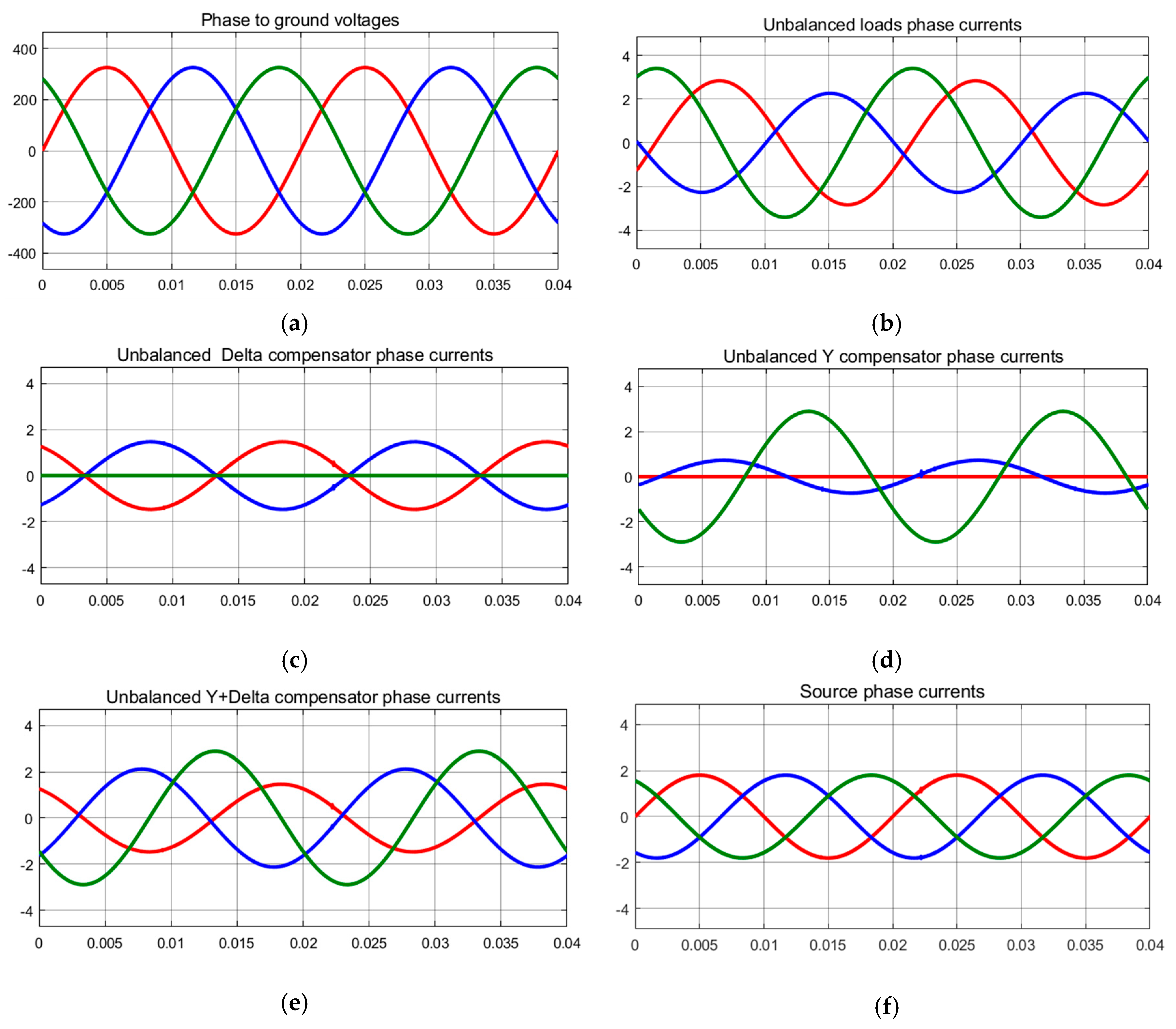
Figure 4.
The results of the experimental determinations: the rms of the phase to neutral voltages, of the currents and the powers on the phases, in the five sections considered of the three-phase circuit.
Figure 4.
The results of the experimental determinations: the rms of the phase to neutral voltages, of the currents and the powers on the phases, in the five sections considered of the three-phase circuit.


Table 1.
The unbalanced three-phase load.
| Component | Equivalent Parameters | Active Powers | Reactive Powers | Phase Currents | Sequence Currents |
|---|---|---|---|---|---|
| Load (Yn) | |||||
| - | - |
Table 2.
The unbalanced compensator sized by the “classical” method (Balancing Reactive Compensator (BRC)).
Table 2.
The unbalanced compensator sized by the “classical” method (Balancing Reactive Compensator (BRC)).
| Component | Equivalent Parameters | Active Powers | Reactive Powers | Phase Currents | Sequence Currents |
|---|---|---|---|---|---|
| Yn | |||||
| - | |||||
| - | |||||
| - | - | - | |||
| Δ | −68.70 | ||||
| - | |||||
| - | |||||
| - | - | - | |||
| Yn + Δ | - | ||||
| - | |||||
| - | |||||
| - | |||||
| - | |||||
| - | - | - |
Table 3.
The unbalanced compensator sized using version 5(3) (Balancing Capacitive Compensator (BCC)).
Table 3.
The unbalanced compensator sized using version 5(3) (Balancing Capacitive Compensator (BCC)).
| Component | Equivalent Parameters | Active Powers | Reactive Powers | Phase Currents | Sequence Currents |
|---|---|---|---|---|---|
| Yn | |||||
| - | |||||
| - | |||||
| - | - | - | |||
| Δ | |||||
| - | |||||
| - | |||||
| - | - | - | |||
| Yn + Δ | - | ||||
| - | |||||
| - | |||||
| - | |||||
| - | |||||
| - | - | - | . |
Table 4.
The assembly load-compensator seen from the network (Point of Common Coupling (PCC)).
| Component | Equivalent Parameters | Real Powers | Reactive Powers | Phase Currents | Sequence Currents |
|---|---|---|---|---|---|
| Network (PCC) | |||||
| - | |||||
| - | |||||
| - | - | - |
© 2018 by the authors. Licensee MDPI, Basel, Switzerland. This article is an open access article distributed under the terms and conditions of the Creative Commons Attribution (CC BY) license (http://creativecommons.org/licenses/by/4.0/).
Share and Cite
MDPI and ACS Style
Pană, A.; Băloi, A.; Molnar-Matei, F. From the Balancing Reactive Compensator to the Balancing Capacitive Compensator. Energies 2018, 11, 1979. https://doi.org/10.3390/en11081979
AMA Style
Pană A, Băloi A, Molnar-Matei F. From the Balancing Reactive Compensator to the Balancing Capacitive Compensator. Energies. 2018; 11(8):1979. https://doi.org/10.3390/en11081979
Chicago/Turabian StylePană, Adrian, Alexandru Băloi, and Florin Molnar-Matei. 2018. "From the Balancing Reactive Compensator to the Balancing Capacitive Compensator" Energies 11, no. 8: 1979. https://doi.org/10.3390/en11081979
Note that from the first issue of 2016, this journal uses article numbers instead of page numbers. See further details here.