Solar Panel Supplier Selection for the Photovoltaic System Design by Using Fuzzy Multi-Criteria Decision Making (MCDM) Approaches

Abstract

The period of industrialization and modernization has increased energy demands around the world. As with other countries, the Taiwanese government is trying to increase the proportion of renewable energy, especially solar energy resources. Thus, there are many solar power plants built in Taiwan. One of the most important components of a solar power plant is the solar panel. The solar panel supplier selection process is a complex and multi-faceted decision that can reduce the cost of purchasing equipment and supply this equipment on time. In this research, we propose fuzzy MCDM approach that includes fuzzy analytical hierarchy process model (FAHP) and data envelopment analysis (DEA) for evaluation and selection of solar panel supplier for a photovoltaic system design in Taiwan. The main objective of this work is to design a fuzzy MCDM approach for solar panel supplier selection based on qualitative and quantitative factors. In the first step of this research, FAHP is applied to define the priority of suppliers. The AHP combined with fuzzy logic (FAHP) can be used to rank suppliers; however, the disadvantages of the FAHP model is that input data, expressed in linguistic terms, depends on experience of experts and the number of suppliers is practically limited, because of the number of pairwise comparison matrices. Thus, we applied several DEA models for ranking potential suppliers in the final stages. As the result, decision making unit 1 (DMU 1) is the optimal solar panel supplier for photovoltaic system design in Taiwan. The contribution of this research is a new fuzzy MCDM for supplier selection under fuzzy environment conditions. This paper also lies in the evolution of a new approach that is flexible and practical to the decision maker. It provides a useful guideline for solar panel supplier selection in many countries as well as a guideline for supplier selection in other industries.

1. Introduction

Nowadays, Taiwan’s fossil fuel resources have been exhausted due to over-exploitation. As other countries, the over-exploitation of fossil fuels leading to exhaustion occurs. Taiwan has been importing materials and primary energy for electricity production, the development of renewable energy will help Taiwan diversify, self-reliant power supply and environmental protection. As Taiwan’s new electricity rates, which come with an average hike of 3 percent, electricity rates will be raised by an average of NT$2.6253 (US$0.09) per kilowatt-hour (kWh). Thus, the government of Taiwan encourages the development of renewable energy, intelligent grid technology, and new energy technologies, as well as studied on how to exploit renewable energy sources.

The reduction in the Emissions of Carbon Dioxide (ERCD) signifies an environmental improvement when a PV system is used as an alternative to a mix of fossil fuels. The sustainability of a PV system is defined also by estimation of the energy and environmental performances [1]. A previous analysis has quantified these values for Italian context: Energy Payback Time (EPBT) is equal to 2.4–3.0 years, Greenhouse Gas Payback Time (GPBT) is equal to 2.5–3.2 years, Energy Return on Investment (EROI) is equal to 6.2–7.9 and Greenhouse Gas Return on Investment is equal to 5.8–7.5 [2]. ERcd permits a comparison between PV source and a mix of fossil fuels. The use of PV helps increase the efficiency of a photovoltaic/energy storage [3]. Especially in the context of the rapidly growing industry that now leads to exhausted fossil fuels, the use of PV is essential.

Therefore, there are many solar power plant are building in Taiwan. One of the most important components of a solar power plant is the solar panel. The process of transferring from a solar cell to a photovoltaic (PV) system is shown in Figure 1.

Sunlight is converted to electricity by solar panels. Photovoltaic modules constitute the photovoltaic array of a system that generates and supplies solar electricity. Each module is rated by its DC output power under standard test conditions, and typically ranges from 100 to 365 W. The efficiency of a module defines the area of a module given the same rated output—an 8% efficient 230 W module will have twice the area of a 16% efficient 230 W module. There are a few commercially available solar modules that exceed efficiency of 24% [4,5]. The process of transferring from a solar cell to a photovoltaic (PV) system is shown in Figure 1.

Nowadays, the price of solar power has fallen to levels that make it cheaper than ordinary fossil fuel based electricity from the electricity grid, a phenomenon known as grid parity [6].

Several studies have used multi-criteria decision making (MCDM) approaches to various fields of science and engineering, and this trend has been increasing for many years. Supplier selection is one of the fields to which the MCDM approach has been applied, yet very few studies consider this problem under fuzzy environmental conditions. Hence, we are motivated to study a proposed fuzzy MCDM approach that includes fuzzy analytical hierarchy process model (FAHP) and data envelopment analysis (DEA) for evaluation and selection of solar panel supplier for a photovoltaic system design in Taiwan. In industrial context this paper investigates how to increase the efficiency of a photovoltaic/energy storage.

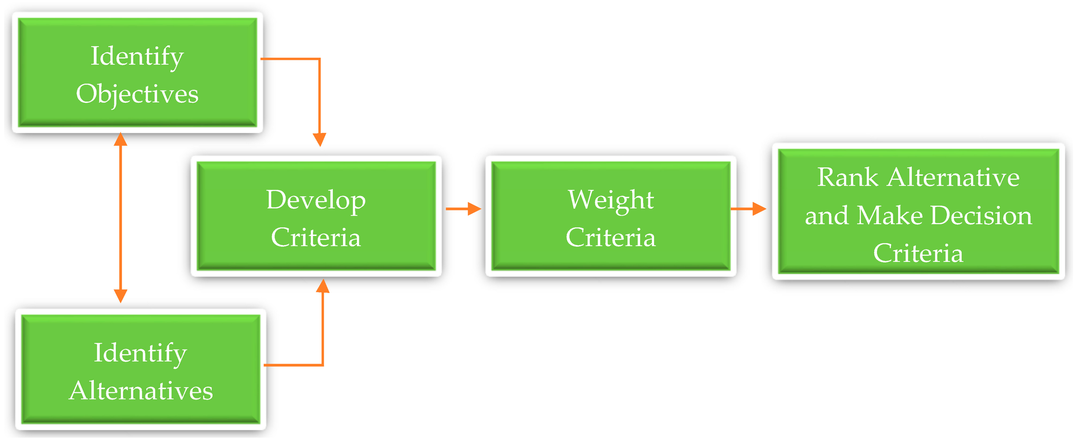
A generic process of MCDM is shown in Figure 2.

In the first stages of this work, FAHP is proposed for determining the priority of suppliers. FAHP is a widely used decision making technique in many MCDM problems and FAHP method is one of the best for determining the weight of criteria and alternatives. The steps for implementing the FANP model are as follows:

Step 1

Calculation of TFN’s

Step 2

Calculation of ${\tilde{Q}}_1$

Step 3

Calculation of ${\tilde{Q}}_Y$

Step 4

Calculation of $\tilde{R}$

Step 5

Calculation of $w{b}_{\beta l}$

Step 6

Calculation of W_bl, W_bz

Step 7

Calculation of X_be

Step 8

Calculation of W_bz.

The FAHP or AHP can be used for ranking suppliers but the disadvantage of the FAHP model is that input data, expressed in linguistic terms, depends on experience of experts. Thus, we applied several DEA models for ranking solar panel suppliers in final stages of this research. The three main phases in carrying out an efficiency study by means of DEA are the following:

Step 1

Definition and selection of DMUs to enter the analysis.

Step 2

Determination of input and output factors which are relevant and suitable for assessing the relative efficiency of the selected DMUs.

Step 3

Application of the DEA models and analysis of outcomes.

An optimal supplier are identified as extreme efficient at all proposed DEA models.

The remainder of the papers provides background materials to assist in developing the fuzzy MCDM approaches. Then, a hybrid FAHP-DEA model is proposed to select solar panel supplier in Taiwan. The results, discussion, and the contributions are presented at the end of the paper.

2. Literature Review

Selecting a supplier is a multi-criteria decision, and complex to find an optimal solution to select the right supplier. Several different critical decision-making methods are identified by the scholarly analysts such as the AHP, ANP, FANP, artificial neural networks (ANN), case based reasoning (CBR), data envelopment analysis (DEA), genetic algorithm (GA), fuzzy set theory, mathematical programming (MP) etc. [7].

The Analytical Hierarchy Process (AHP), also known as hierarchical analysis, was studied and developed by Thomas L. Saaty [8]. Bisides, Ghodsypour et al. [9] consider both tangible and intangible factors in choosing the best suppliers and placing the optimum order quantities among them such that the total value of purchasing (TVP) becomes maximum. The comparision of the total cost of ownership and analytic hierarchy process approaches to solve supplier selection was proposed by Bhutta [10]. Mohanty et al. [11] presented an application of analytic hierarchic process (AHP) for evaluating the sources of supply in a materials management situation. The AHP has used to structure the supplier selection procedure [12] and Weber et al. [13] given to the criteria and analytical methods used in the vendor selection process. Applied AHP method to rate vendor was done by Kingsman [14]. Nakagawa and Sekitani [15] addressed a new use of ANP on SCM strategic decision analysis such as a supplier selection and improvement of supply chain performance. Handfield et al. [16] used the AHP to evaluate the relative importance of various environmental traits and to assess the relative performance of several suppliers along these traits. Agarwal and Shanker [17] proposed an analytic network process (ANP) to analyze alternatives for improvement in supply chain performance. Besides, Sarkis and Sundarraj [18] showed ANP model combined with an optimization model can be used to conduct a comprehensive evaluation of these varied issues. Sarkis and Talluri [19] addresses the supplier selection with multiple factors.

A hybrid model including Fuzzy Analytical Hierarchy Process (FAHP), Fuzzy TOPSIS, and AHP, Axiomatic Design (AD) and Data Envelopment Analysis (DEA) to evaluate and selection suppliers proposed by Alptekin Ulutas et al. [20]. An integrated FAHP-DEA for multiple criteria ABC inventory classification by A.Hadi-Vencheh [21]. Develop a novel performance evaluation method, which integrates both FAHP method and fuzzy DEA for assisting organisations to make the supplier selection decision in auto lighting OEM company by R.J.Kou [22]. A hybrid FAHP-AR-DEA to assess the efficiencies of PV solar plant site candidates by Amy H. I. Lee et al. [23]. A integrated TFN-AHP-DEA approaches for renewable energy projects analyzed economic feasibility by Gan et al. [24]. A supplier performance evaluation model based on AHP and DEA by He-Yau-Kang [25]. A hybrid model including DEA-FAHP-TOPSIS for solar power plant location selection in Viet Nam by Chia-Nan Wang [26]. Figen Balo [27] proposed the selection of the best solar panel for the photovoltaic system design by using AHP. A hybrid model DEA—FANP for supporting the department selection process within Iran Amirkabir University by Babak Daneshvar Rouyendegh et al. [28]. A hybrid FANP-DEA approach for supplier evaluation and selection by Chia-Nan Wang [29]. In study GIS and FAHP for land analysis in Solar Farms by Ehsan Noorollahi [30]. An AHP to weight the criteria, whereas fuzzy TOPSIS was applied for the installation of solar ther-moelectric power plants on the coast of Murcia, Spain by Sánchez et al. [31]. A model with DEA and Malmquist index was constructed to evaluate the total factor energy efficiency (TFEE) in thermal power industry by Jin-Peng Liu [32]. An analytic network process (ANP) for selection of photovoltaic (PV) solar power projects by Pablo Aragones Beltran [33]. A decision and methodology to locate potential sites for large-scale Solar PV (SPV) plants focusing on various factors based on GIS by Ghazanfar Khan [34].

A hybrid approaches as improvements for decision-making related to sustainability issues, while also promoting future application of the approaches by Edmundas Kazimieras Zavadskas [35]. In study reviewed of applications of MADM approaches for evaluation and selection of suppliers in a fuzzy environment by Mehdi Keshavarz Ghorabaee [36]. The solar panel for the photovoltaic system design by using AHP model by Figen Balo [27]. A hybrid model including GIS-DEM-AHP to identify the most suitable location for the installation of solar panel power plant in the Municipality of Knjaževac (East Serbia) by I. Potić et al. [37]. In study applied SWOT and Fuzzy Goal Programming to evaluating the strategies of compressed natural gas industry in Iran by Khan MI [38]. A Grey model and Decision Making Trial and Evaluation Laboratory (DEMATEL) to find out critical factors of green business failure L. Cui [39]. A new model based on the IFS and ANP technique to evaluate the critical factors of the application of nanotechnology in the construction industry by Shahram Shariati et al. [40]. A hybrid Multi-Criteria Decision Making (MCDM) approaches for strategic project portfolio selection of agro by products by Animesh Debnath et al. [41]. An integrated approach QFD-MCDM for green supplier selection by Morteza Yazdani [42]. A R’AMATEL-MAIRCA methods to evaluating the performance of suppliers in green supply chain implementation in electronics industry by Kajal Chatterjee [43]. A MCDM method by combining Analytical Hierarchal Process (AHP) and VlseKriterijuska Optimizacija I Komoromisno Resenje (VIKOR) methods under intervalvalued fuzzy environment to rank of sustainable manufacturing strategies by Sujit Singh et al. [44]. A multi-criteria group decision support based on the PROMETHEE method, which clearly depicts conflicting targets of decision-makers, and thus supports articulating criteria, preferences and weights of various stakeholders by Ute Weißfloch [45]. A decision framework of photovoltaic module selection under interval-valued intuitionistic fuzzy environment by Shengping Long [46]. A analytical hierarchy process (AHP) model identifying the weights of criteria in the MCDM problem by Halil I. Cobuloglu [47]. The MCDM approaches based on the Ratio system part of the MOORA method, which should enable an efficient selection of the adequate comminution circuit design by D. Stanujkic [48]. A hybrid MCDM model to addresses dependent relationships between various criteria and the vague information coming from decision-makers for improving and selecting suppliers in green supply chain management by James J.H. Liou [49]. A MCDM model for supplier selection in the construction company by Željko Stevi’c [50]. A hybrid BWM and Znumbers, namely ZBWM in supplier development by Hamed Aboutorab et al. [51]. A MCDM model for selection of suppliers in a company producing polyvinyl chloride (PVC) carpentry proposed by Gordan Stoji´c et al. [52].

3. Materials and Methods

3.1. Research Development

Figure 3 illustrates the solar panel supplier selection process which is sequentially presented in three stages.

Stage 1: Defining criteria. Initially, we define the criteria and sub criteria that affect the solar panel supplier selection, by interviewing experts, and performing a literature review of the research.

Stage 2: In this stage, we combined the Analytical Hierarchy Process (AHP) with fuzzy logic to overcome the disadvantages of the AHP method. Thus, the FAHP model is the best technique for addressing complex problems of decision-making, which has a connection with various qualitative and quantitative attributes. In this work, FAHP is applied to determine the priority of all potential suppliers.

Stage 3: Applying several DEA models. In this step, all potential suppliers are ranked by several DEA models including BCC models, SBM models, and super SBM models.

3.2. Methodology

3.2.1. Fuzzy Sets and Fuzzy Number

Zadeh (1965) [53] introduced the theory to deal with uncertainty environment conditions. A value of the membership function of fuzzy set is between [0, 1] [54,55]. The triangular fuzzy number (TFN) can be defined as (a, b, c). The value a, b and c (a ≤ b ≤ c), indicate the smallest, the promising and the largest value. A TFN is shown in Figure 4.

Triangular fuzzy number can be describe as:

$$\mu \left(\frac{x}{\tilde{F}}\right)=\{\begin{array}{c}0,\\ \frac{x-a}{b-a}\\ \frac{c-x}{c-b}\\ 0,\end{array} \begin{array}{c}x<a,\\ a\le x\le b,\\ b\le x\le c,\\ x>c,\end{array}$$

(1)

A fuzzy number (FN) is given by the representatives of each level of membership function as following:

$$\tilde{F}=(F^{l\left(y\right)},F^{r\left(y\right)})=\left[a+\left(b-a\right)y, c+\left(b-c\right)y\right],y \in \left[0,1\right]$$

(2)

F(y), F(y) indicates both the left and the right side of a NF. Two positive TFN (a₁, b₁, c₁) and (a₁, b₂, c₂) are presented as following:

$$\begin{gathered} \left(a_1, b_1, c_1\right)+\left(a_2, b_2, c_2\right)=\left(a_1+a_2, b_1+b_2,c_1+c_2\right) \\ \left(a_1, b_1, c_1\right)-\left(a_2, b_2, c_2\right)=\left(a_1-a_2, b_1-b_2,c_1-c_2\right) \\ \left(a_1, b_1, c_1\right)\times \left(a_2, b_2, c_2\right)=\left(a_1\times a_2, b_1\times b_2,c_1\times c_2\right) \\ \frac{\left(a_1, b_1, c_1\right)}{\left(a_2, b_2, c_2\right)}=\left(a_1/c_2, b_1/b_2,c_1/a_2\right) \end{gathered}$$

(3)

3.2.2. Fuzzy Analytical Hierarchy Process (AHP)

Analytic Hierarchy Process (FAHP) embeds the fuzzy theory to basic Analytic Hierarchy Process (AHP), which was developed by Saaty [8]. FAHP is a widely used decision making technique in many MCDM problems. In a general AHP model, the objective is in the first level, the criteria and sub criteria are in the second and third levels respectively. Finally the options are found in the fourth level [56].

There are seven steps of the FAHP procedure as following:

Step 1 Decision-maker compares the criteria or alternatives via linguistic terms as shown in

Table 1. Linguistic terms and the corresponding TFN.

Saaty Scale	Definition	FTN Scale
1	Equally important	(1,1,1)
3	Weakly important	(2,3,4)
5	Fairly important	(4,5,6)
7	Strongly important	(6,7,8)
9	Absolutely important	(9,9,9)
2	The intermittent values between two adjacent scales	(1,2,3)
4		(3,4,5)
6		(5,6,7)
8		(7,8,9)

.

Step 2 Calculation of ${\tilde{Q}}_1$

A pairwise comparison and relative scores as:

$$\widetilde{Q_b}=\left(l_b,m_b,u_b\right)$$

(4)

$$l_b={\left(l_{b1}\otimes l_{b2}\otimes \dots \otimes l_{bi}\right)}^{\frac{1}{i}}, b=1, 2, \dots i$$

(5)

$$m_b={\left(m_{b1}\otimes m_{b2}\otimes \dots \otimes m_{bi}\right)}^{\frac{1}{i}}, b=1, 2, \dots i$$

(6)

$$u_b={\left(u_{b1}\otimes u_{b2}\otimes \dots \otimes u_{bi}\right)}^{\frac{1}{i}}, b=1, 2, \dots i$$

(7)

Step 3 Calculation of ${\tilde{Q}}_Y$

The geometric fuzzy mean was established by (28):

$${\tilde{Q}}_Y= \left({\displaystyle \sum }_{b=1}^i{l}_b,{\displaystyle \sum }_{b=1}^i{m}_b,{\displaystyle \sum }_{b=1}^i{u}_b\right)$$

(8)

Step 4 Calculation of $\tilde{R}$

The fuzzy geometric mean was determined as:

$$\tilde{R}=\frac{{\tilde{Q}}_b}{{\tilde{Q}}_Y}=\frac{\left(l_b,m_b,u_b\right)}{{{\displaystyle \sum }}_{b=1}^i{l}_b,{{\displaystyle \sum }}_{b=1}^i{m}_b,{{\displaystyle \sum }}_{b=1}^i{u}_i}=\left[\frac{l_b}{{{\displaystyle \sum }}_{b=1}^i{u}_b},\frac{m_b}{{{\displaystyle \sum }}_{b=1}^i{m}_b},\frac{u_b}{{{\displaystyle \sum }}_{b=1}^i{l}_b}\right]$$

(9)

Step 5 Calculation of $W{b}_{\mathsf{\mu }l}$

The criteria depending on $\mathsf{\mu }$ cut values are defined for the calculated β. The fuzzy priorities will apply for lower and upper bounds for each $\mathsf{\mu }$ value:

$$W{b}_{\mathsf{\mu }l}=\left(Wb{l}_{\mathsf{\mu }l},Wb{u}_{\mathsf{\mu }l}\right); b=1, 2, \dots i; l=1, 2, \dots L$$

(10)

Step 6 Calculation of W_bl, W_bu

Values of W_bl, W_bu are calculated by combining the lower and the upper values, and dividing them by the total μ values:

$$W_{bl}=\frac{{{\displaystyle \sum }}_{b=1}^i\mathsf{\mu }{\left(W_{bl}\right)}_l}{{{\displaystyle \sum }}_{l=1}^L{\mathsf{\mu }}_l};b=1, 2, \dots i;l=1, 2, \dots L$$

(11)

$$W_{bu}=\frac{{{\displaystyle \sum }}_{b=1}^i\mathsf{\mu }{\left(W_{bu}\right)}_l}{{{\displaystyle \sum }}_{l=1}^L{\mathsf{\mu }}_l};b=1, 2, \dots i;l=1, 2, \dots L$$

(12)

Step 7 Calculation of X_bd

Combining the upper and the lower bounds values by using the optimism index ($\alpha$) to order to defuzzify:

$$W_{bd}=\alpha \times W_{bu}+\left(1-\mathsf{\alpha }\right)\times W_{bl};\alpha \in \left[0,1\right];b=1,2,\dots i$$

(13)

Step 8 Calculation of W_bz

The defuzzification values priorities are normalization by:

$$W_{bz}=\frac{W_{bd}}{{{\displaystyle \sum }}_{b=1}^i{W}_{bd}};b=1,2,...i$$

(14)

3.2.3. Data Envelopment Analysis (DEA) Model

(1) Banker Charnes Cooper Model (BCC Model)

The input-oriented BCC (BCC-I) model proposed by Bankeretal [57,58], which is able to evaluate the efficiency of DMU₀ by solving the following linear program (LP) [58]:

$$\begin{array}{c}{\delta }_B=\min \delta \\ \mathrm{S}.\mathrm{t}\\ {\displaystyle {\displaystyle \sum }_{j=1}^n}{a}_{ij}{\phi }_j+t_i^{-}=\delta a_{i0},i=1,2,\dots ,p\\ {\displaystyle {\displaystyle \sum }_{j=1}^n}{b}_{rj}{\phi }_j-t_r^{+}=b_{r0},r=1,2,\dots ,q\\ {\displaystyle {\displaystyle \sum }_{k=1}^n}{\phi }_k=1\\ {\phi }_k\ge 0,k=1,2,\dots ,n\end{array}$$

(15)

Some boundary points may be “weakly efficient” because we have nonzero slacks. However, we can avoid being worried even in such cases by invoking the following linear program in which the slacks are taken to their maximal values [58]:

$$\begin{array}{c}\max {\displaystyle {\displaystyle \sum }_{i=1}^m}{t}_i^{-}+{\displaystyle {\displaystyle \sum }_{r=1}^t}{t}_r^{+}\\ \mathrm{S}.\mathrm{t}\\ {\displaystyle {\displaystyle \sum }_{j=1}^n}{a}_{ij}{\phi }_j+d_i^{-}=\delta a_{i0},i=1,2,\dots ,p\\ {\displaystyle {\displaystyle \sum }_{j=1}^n}{b}_{rj}{\phi }_j-t_r^{+}=b_{r0},r=1,2,\dots ,q\\ {\displaystyle {\displaystyle \sum }_{k=1}^n}{\phi }_k=1\\ {\phi }_k\ge 0,k=1,2,\dots ,n\\ t_i^{-}\ge 0,i=1,2,\dots ,p\\ t_r^{+}\ge 0,r=1,2,\dots ,q\end{array}$$

(16)

Therefore, it is to be noted that the preceding development amounts to solving the following problem in two steps [58]

$$\begin{array}{c}\min \delta -\epsilon \left({\displaystyle {\displaystyle \sum }_{i=1}^m}{t}_i^{-}+{\displaystyle {\displaystyle \sum }_{r=1}^t}{t}_r^{+}\right)\\ \mathrm{S}.\mathrm{t}\\ {\displaystyle {\displaystyle \sum }_{j=1}^n}{a}_{ij}{\phi }_j+t_i^{-}=\delta a_{i0},i=1,2,\dots ,p\\ {\displaystyle {\displaystyle \sum }_{j=1}^n}{b}_{rj}{\phi }_j-t_r^{+}=b_{r0},r=1,2,\dots ,q\\ {\displaystyle {\displaystyle \sum }_{k=1}^n}{\phi }_k=1\\ {\phi }_k\ge 0,k=1,2,\dots ,n\\ t_i^{-}\ge 0,i=1,2,\dots ,p\\ t_r^{+}\ge 0,r=1,2,\dots ,q\end{array}$$

(17)

The dual multiplier form of the linear program (17) is expressed as [58]:

$$\begin{array}{c}\underset{g.f,f_0}{\max }{\delta }_B=e^V{b}_0-e_0\\ \mathrm{S}.\mathrm{t}\\ g^V{a}_0=1\\ e^V{b}_j-g^V{a}_j-e_0\le 0, j=1, 2,\dots ,n\\ g\ge 0\\ e\ge 0\end{array}$$

(18)

The scalar v₀ may be positive or negative (or zero). The equivalent BCC fractional program is obtained from the dual program (18) as [58]:

$$\begin{array}{c}\underset{g.e}{\max }\delta =\frac{e^V{b}_0-e_0}{g^V{a}_0}\\ \mathrm{S}.\mathrm{t}\\ \frac{e^V{b}_j-e_0}{g^V{a}_j}\le 1,j=1,2,\dots ,n\\ g\ge 0\\ e\ge 0\end{array}$$

(19)

The improved activity $\left({\delta }^{*}a-t^{-*},b+t^{+*}\right)$ also can be illustrated as BCC efficient [58]. The output-oriented BCC model (BCC-O) is:

$$\begin{array}{c}\max \eta \\ \mathrm{S}.\mathrm{t}\\ {\displaystyle {\displaystyle \sum }_{j=1}^n}{a}_{ij}{\phi }_j+t_i^{-}=\delta a_{i0},i=1,2,\dots ,p\\ {\displaystyle {\displaystyle \sum }_{j=1}^n}{b}_{rj}{\phi }_j-t_r^{+}=\eta b_{r0},r=1,2,\dots ,q\\ {\displaystyle {\displaystyle \sum }_{k=1}^n}{\phi }_k=1\\ {\phi }_k\ge 0,k=1,2,\dots ,n\end{array}$$

(20)

We have the associate multiplier form, which is expressed as [58]:

$$\begin{array}{c}\underset{g.f,g_0}{\min }{e}^V{b}_0-e_0\\ \mathrm{S}.\mathrm{t}\\ e^V{b}_0=1\\ g^V{a}_j-e^V{b}_j-e_0\le 0,j=1,2,\dots ,n\\ g\ge 0\\ e\ge 0\end{array}$$

(21)

The f₀ is the scalar associated with ${\displaystyle \sum }_{k=1}^n{\phi }_k=1$. The equivalent (BCC) fractional programming formulation for model (20) as bellows [58]:

$$\begin{array}{c}\underset{g.e,g_0}{\min }\frac{g^V{a}_0-e_0}{e^V{b}_0}\\ \mathrm{S}.\mathrm{t}\\ \frac{e^V{a}_j-e_0}{e^V{b}_j}\le 1,j=1,2,\dots ,n\\ g\ge 0\\ e\ge 0\end{array}$$

(22)

(2) Input—Oriented Slacks Based Measure (SBM-I-C)

Input—oriented SBM under constant-returns-to-scale assumption [58]:

$$\begin{array}{c}{\rho }_I^{*}=\underset{\beta , t^{-},t^{+}}{\min }1-\frac{1}{m}{\displaystyle {\displaystyle \sum }_{i=1}^m}\frac{t_i^{-}}{a_{ih}}\\ \mathrm{S}.\mathrm{t}\\ x_{ic}={\displaystyle {\displaystyle \sum }_{j=1}^m}{a}_{ic}{\phi }_i+t_i^{-},i=1,2,\dots m\\ y_{rc}={\displaystyle {\displaystyle \sum }_{j=1}^m}{b}_{rc}{\phi }_i-t_r^{+},i=1,2,\dots d\\ {\phi }_j\ge 0,k\left(\forall j\right),t_i^{-}\ge 0\left(\forall j\right),t_r^{+}\ge 0\left(\forall j\right)\end{array}$$

(23)

(3) Output—Oriented SBM (SBM-O-C)

The output-oriented SBM efficiency ${\rho }_O^{*}$ of DMU_c = (a_c, b_c) is defined by [SBM-O-C] [58]:

$$\begin{array}{c}\raisebox{1ex}{$1$}\!\left/ \!\raisebox{-1ex}{${\rho }_O^{*}$}\right.=\underset{\lambda ,t^{-},t^{+}}{\max }1+\frac{1}{t}{\displaystyle \sum }_{r=1}^t\frac{t_r^{+}}{b_{rh}}\\ \mathrm{S}.\mathrm{t}\\ x_{ic}={\displaystyle {\displaystyle \sum }_{j=1}^n}{a}_{ij}{\phi }_j+ t_j^{-}\left(i=1,...m\right)\\ y_{ic}={\displaystyle \sum }_{j=1}^n{b}_{ij}{\phi }_j+t_i^{+}\left(i=1,\dots m\right)\\ {\phi }_j\ge 0\left(\forall j\right), t_i^{-}\ge 0\left(\forall i\right), t_i^{+}\ge 0 \left(\forall r\right)\end{array}$$

(24)

optimal solution of [SBM-O-C] be (${\phi }^{*},t^{-*},t^{+*})$

(4) Super Slacks Based Measure Model

Tone [59] has proposed a super SBM model that measures the efficiency of the units under evaluation using slack variables only.

$$\begin{array}{c}\min {\theta }_q^{SBM}= \frac{\frac{1}{p}{{\displaystyle \sum }}_{i=1}^m{a}_i^{*}/x_{i0}}{\frac{1}{q}{{\displaystyle \sum }}_{k=1}^r{b}_k^{*}/b_{k0}}\\ \mathrm{S}.\mathrm{t}\\ {\displaystyle {\displaystyle \sum }_{j=1}^n}{a}_{ij}{\phi }_j+t_i^{-}=\delta a_{i0},i=1,2,\dots ,p\\ {\displaystyle {\displaystyle \sum }_{j=1}^n}{b}_{rj}{\phi }_j-t_r^{+}=b_{r0},r=1,2,\dots ,q\\ a_i^{*}\ge a_{i0},i=1,2,\dots ,n\\ b_k^{*}\le b_{k0},k=1,2,\dots ,n\\ {\phi }_k\ge 0,k=1,2,\dots ,n\\ t_i^{-}\ge 0,i=1,2,\dots ,p\\ t_r^{+}\ge 0,r=1,2,\dots ,q\end{array}$$

(25)

4. Results

The solar panel is the most important equipment in solar power plants. Solar panel supplier selection process is a complex and multi-faceted decision that can reduce the cost of purchasing equipment and supply equipment on time. Thus, the main objectives of this research is a proposed fuzzy MCDM model for supplier selection based on quality of services, product, risk managements, and suppliers’ characteristics. 15 potential suppliers were selectied by interviewing experts based on quality of Solar panel, product capacity, delivery time, guarantee term, supplier’s location, unit price … in

Table 2. The symbol of 15 solar panel suppliers.

No	Name	Symbol
1	Supplier 1	DMU 1
2	Supplier 2	DMU 2
3	Supplier 3	DMU 3
4	Supplier 4	DMU 4
5	Supplier 5	DMU 5
6	Supplier 6	DMU 6
7	Supplier 7	DMU 7
8	Supplier 8	DMU 8
9	Supplier 9	DMU 9
10	Supplier 10	DMU 10
11	Supplier 11	DMU 11
12	Supplier 12	DMU 12
13	Supplier 13	DMU 13
14	Supplier 14	DMU 14
15	Supplier 15	DMU 15

.

The hierarchical structures of the FAHP model is shown in Figure 5.

A fuzzy comparison matrices of criteria and sub criterial are shown in

Table 3. Fuzzy comparison matrices for criteria.

Criteria	A	B	C	D
A	(1,1,1)	(1/4,1/3,1/2)	(1/4,1/3,1/2)	(1,2,3)
B	(2,3,4)	(1,1,1)	(3,4,5)	(4,5,6)
C	(2,3,4)	(1/5,1/4,1/3)	(1,1,1)	(3,4,5)
D	(1/3,1/2,1)	(1/6,1/5,1/4)	(1/5,1/4,1/3)	(1,1,1)

,

Table 4. Real number priority.

Criteria	A	B	C	D
A	1	1/3	1/3	2
B	3	1	4	5
C	3	1/4	1	4
D	1/2	1/5	1/4	1

,

Table 5. Fuzzy comparison matrices for criteria.

Criteria	A	B	C	D	Weight
A	(1,1,1)	(1/4,1/3,1/2)	(1/4,1/3,1/2)	(1,2,3)	0.13
B	(2,3,4)	(1,1,1)	(3,4,5)	(4,5,6)	0.56
C	(2,3,4)	(1/5,1/4,1/3)	(1,1,1)	(3,4,5)	0.25
D	(1/3,1/2,1)	(1/6,1/5,1/4)	(1/5,1/4,1/3)	(1,1,1)	0.08
Total
CR = 0.089

,

Table 6. Comparison matrix for A.

Criteria	A1	A2	A3	A4
A1	(1,1,1)	(1/4,1/3,1/2)	(3,4,5)	(2,3,4)
A2	(2,3,4)	(1,1,1)	(4,5,6)	(3,4,5)
A3	(1/5,1/4,1/3)	(1/6,1/5,1/4)	(1,1,1)	(1/3,1/2,1)
A4	(1/4,1/3,1/2)	(1/5,1/4,1/3)	(1,2,3)	(1,1,1)
Total
CR = 0.04288

,

Table 7. Comparison matrix for B.

Criteria	B1	B2	B3	B4
B1	(1,1,1)	(1/5,1/4,1/3)	(2,3,4)	(3,4,5)
B2	(3,4,5)	(1,1,1)	(4,5,6)	(3,4,5)
B3	(1/4,1/3,1/2)	(1/6,1/5,1/4)	(1,1,1)	(1/3,1/2,1)
B4	(1/5,1/4,1/3)	(1/5,1/4,1/3)	(1,2,3)	(1,1,1)
Total				1
CR = 0.09312

,

Table 8. Comparison matrix for C.

Criteria	C1	C2	C3	Weight
C1	(1,1,1)	(3,4,5)	(2,3,4)	0.625013074
C2	(1/5,1/4,1/3)	(1,1,1)	(1/3,1/2,1)	0.136499803
C3	(1/4,1/3,1/2)	(1,2,3)	(1,1,1)	0.238487123
Total
CR = 0.01759

,

Table 9. Comparison matrix for D.

	D1	D2	D3	D4
D1	(1,1,1)	(2,3,4)	(3,4,5)	(5,6,7)
D2	(1/4,1/3,1/2)	(1,1,1)	(3,4,5)	(2,3,4)
D3	(1/5,1/4,1/3)	(1/5,1/4,1/3)	(1,1,1)	(1,2,3)
D4	(1/7,1/6,1/5)	(1/4,1/3,1/2)	(1/3,1/2,1)	(1,1,1)
Total
CR = 0.0577

,

Table 10. Comparision matrix of S1 based on Sub-criteria.

Sub-Criteria	A1	A2	A3	A4	B1	B2	B3	B4	C1	C2	C3	D1	D2	D3	D4	Weight
A1	(1,1,1)	(1/7,1/6,1/5)	(3,4,5)	(4,5,6)	(5,6,7)	(4,5,6)	(1,1,1)	(2,3,4)	(3,4,5)	(4,5,6)	(2,3,4)	(4,5,6)	(7,8,9)	(5,6,7)	(2,3,4)	0.190051
A2	(1/7,1/6,1/5)	(1,1,1)	(1/3,1/2,1)	(1/3,1/2,1)	(1/3,1/2,1)	(1,1,1)	(1/5,1/4,1/3)	(1/4,1/3,1/2)	(1/3,1/2,1)	(1/3,1/2,1)	(1/5,1/4,1/3)	(2,3,4)	(3,4,5)	(3,4,5)	(4,5,6)	0.038205
A3	(1/5,1/4,1/3)	(1/3,1/2,1)	(1,1,1)	(2,3,4)	(5,6,7)	(4,5,6)	(1,2,3)	(1,1,1)	(1,2,3)	(6,7,8)	(1,2,3)	(5,6,7)	(4,5,6)	(3,4,5)	(2,3,4)	0.129681
A4	(1/6,1/5,1/4)	(1/3,1/2,1)	(1/4,1/3,1/2)	(1,1,1)	(1,2,3)	(3,4,5)	(1/5,1/4,1/3)	(1/4,1/3,1/2)	(1,2,3)	(2,3,4)	(1/3,1/2,1)	(1,2,3)	(4,5,6)	(1,2,3)	(3,4,5)	0.061474
B1	(1/7,1/6,1/5)	(1/3,1/2,1)	(1/7,1/6,1/5)	(1/3,1/2,1)	(1,1,1)	(2,3,4)	(1/5,1/4,1/3)	(1/4,1/3,1/2)	(1/3,1/2,1)	(1/3,1/2,1)	(1/5,1/4,1/3)	(1,2,3)	(3,4,5)	(1,2,3)	(4,5,6)	0.038731
B2	(1/6,1/5,1/4)	(1,1,1)	(1/6,1/5,1/4)	(1/5,1/4,1/3)	(1/4,1/3,1/2)	(1,1,1)	(1/4,1/3,1/2)	(1/5,1/4,1/3)	(1/6,1/5,1/4)	(1/3,1/2,1)	(1/5,1/4,1/3)	(1,1,1)	(2,3,4)	(3,4,5)	(1,2,3)	0.027173
B3	(1,1,1)	(3,4,5)	(1/3,1/2,1)	(3,4,5)	(3,4,5)	(2,3,4)	(1,1,1)	(1/3,1/2,1)	(1/7,1/6,1/5)	(2,3,4)	(1,2,3)	(4,5,6)	(6,7,8)	(4,5,6)	(5,6,7)	0.128641
B4	(1/4,1/3,1/2)	(2,3,4)	(1,1,1)	(2,3,4)	(2,3,4)	(3,4,5)	(1,2,3)	(1,1,1)	(1/4,1/3,1/2)	(1,2,3)	(1,2,3)	(3,4,5)	(6,7,8)	(6,7,8)	(3,4,5)	0.113237
C1	(1/5,1/4,1/3)	(1,2,3)	(1/3,1/2,1)	(1/3,1/2,1)	(1,2,3)	(4,5,6)	(1/7,1/6,1/5)	(1/4,1/3,1/2)	(1,1,1)	(1,2,3)	(1/3,1/2,1)	(4,5,6)	(3,4,5)	(4,5,6)	(5,6,7)	0.063599
C2	(1/6,1/5,1/4)	(1,2,3)	(1/8,1/7,1/6)	(1/4,1/3,1/2)	(1,2,3)	(1,2,3)	(1/4,1/3,1/2)	(1/3,1/2,1)	(1/3,1/2,1)	(1,1,1)	(2,3,4)	(5,6,7)	(3,4,5)	(3,4,5)	(4,5,6)	0.061793
C3	(1/4,1/3,1/2)	(3,4,5)	(1/3,1/2,1)	(1,2,3)	(3,4,5)	(3,4,5)	(1/3,1/2,1)	(1/3,1/2,1)	(1,2,3)	(1/4,1/3,1/2)	(1,1,1)	(2,3,4)	(2,3,4)	(1,2,3)	(3,4,5)	0.071764
D1	(1/6,1/5,1/4)	(1/4,1/3,1/2)	(1/7,1/6,1/5)	(1/3,1/2,1)	(1/3,1/2,1)	(1,1,1)	(1/6,1/5,1/4)	(1/5,1/4,1/3)	(1/6,1/5,1/4)	(1/7,1/6,1/5)	(1/4,1/3,1/2)	(1,1,1)	(1,2,3)	(4,5,6)	(1,2,3)	0.024934
D2	(1/9.1/8,1/7)	(1/5,1/4,1/3)	(1/6,1/5,1/4)	(1/6,1/5,1/4)	(1/5,1/4,1/3)	(1/4,1/3,1/2)	(1/8,1/7,1/6)	(1/8,1/7,1/6)	(1/5,1/4,1/3)	(1/5,1/4,1/3)	(1/4,1/3,1/2)	(1/3,1/2,1)	(1,1,1)	(2,3,4)	(1,1,1)	0.016156
D3	(1/7,1/6,1/5)	(1/5,1/4,1/3)	(1/5,1/4,1/3)	(1/3,1/2,1)	(1/3,1/2,1)	(1/5,1/4,1/3)	(1/6,1/5,1/4)	(1/8,1/7,1/6)	(1/6,1/5,1/4)	(1/5,1/4,1/3)	(1/3,1/2,1)	(1/6,1/5,1/4)	(1/4,1/3,1/2)	(1,1,1)	(1,2,3)	0.017355
D4	(1/4,1/3,1/2)	(1/6,1/5,1/4)	(1/4,1/3,1/2)	(1/5,1/4,1/3)	(1/6,1/5,1/4)	(1/3,1/2,1)	(1/7,1/6,1/5)	(1/5,1/4,1/3)	(1/7,1/6,1/5)	(1/6,1/5,1/4)	(1/5,1/4,1/3)	(1/3,1/2,1)	(1,1,1)	(1/3,1/2,1)	(1,1,1)	0.017206
Total																1
CR = 0.0998

The remaining alternatives do the same as Table 10.

and

Table 11. Comparision matrix of A1 based on Alternatives.

	S1	S2	S3	S4	S5	S6	S7	S8	S9	S10	S11	S12	S13	S14	S15	Weight
S1	(1,1,1)	(3,4,5)	(3,4,5)	(4,5,6)	(2,3,4)	(4,5,6)	(4,5,6)	(3,4,5)	(1,2,3)	(2,3,4)	(1,2,3)	(5,6,7)	(1,2,3)	(4,5,6)	(1,2,3)	0.171292
S2	(1/5,1/4,1/3)	(1,1,1)	(1/5,1/4,1/3)	(1,1,1)	(1/4,1/3,1/2)	(3,4,5)	(2,3,4)	(3,4,5)	(1/3,1/2,1)	(1,2,3)	(1,2,3)	(1,2,3)	(2,3,4)	(2,3,4)	(1/5,1/4,1/3)	0.060692
S3	(1/5,1/4,1/3)	(3,4,5)	(1,1,1)	(1,2,3)	(1,2,3)	(3,4,5)	(5,6,7)	(3,4,5)	(3,4,5)	(1,2,3)	(4,5,6)	(5,6,7)	(2,3,4)	(2,3,4)	(1/3,1/2,1)	0.124023
S4	(1/6,1/5,1/4)	(1,1,1)	(1/3,1/2,1)	(1,1,1)	(1,2,3)	(1/3,1/2,1)	(1,2,3)	(3,4,5)	(1/3,1/2,1)	(1,2,3)	(4,5,6)	(1/3,1/2,1)	(1,1,1)	(2,3,4)	(1/6,1/5,1/4)	0.055432
S5	(1/4,1/3,1/2)	(2,3,4)	(1/3,1/2,1)	(1/3,1/2,1)	(1,1,1)	(2,3,4)	(1,2,3)	(3,4,5)	(1/3,1/2,1)	(1,2,3)	(3,4,5)	(4,5,6)	(2,3,4)	(2,3,4)	(1/4,1/3,1/2)	0.078843
S6	(1/6,1/5,1/4)	(1/5,1/4,1/3)	(1/5,1/4,1/3)	(1,2,3)	(1/4,1/3,1/2)	(1,1,1)	(1,2,3)	(1,1,1)	(1/5,1/4,1/3)	(1,2,3)	(1,2,3)	(1,1,1)	(1,1,1)	(2,3,4)	(1/4,1/3,1/2)	0.039954
S7	(1/6,1/5,1/4)	(1/4,1/3,1/2)	(1/7,1/6,1/5)	(1/3,1/2,1)	(1/3,1/2,1)	(1/3,1/2,1)	(1,1,1)	(1/3,1/2,1)	(1/4,1/3,1/2)	(1/5,1/4,1/3)	(1/5,1/4,1/3)	(1/5,1/4,1/3)	(1/3,1/2,1)	(1/4,1/3,1/2)	(1/7,1/6,1/5)	0.017856
S8	(1/5,1/4,1/3)	(1/5,1/4,1/3)	(1/5,1/4,1/3)	(1/5,1/4,1/3)	(1/5,1/4,1/3)	(1,1,1)	(1,2,3)	(1,1,1)	(1/5,1/4,1/3)	(1/3,1/2,1)	(3,4,5)	(1/4,1/3,1/2)	(1/4,1/3,1/2)	(1,2,3)	(1/5,1/4,1/3)	0.027759
S9	(1/3,1/2,1)	(1,2,3)	(1/5,1/4,1/3)	(1,2,3)	(1,2,3)	(3,4,5)	(2,3,4)	(3,4,5)	(1,1,1)	(1,2,3)	(2,3,4)	(2,3,4)	(2,3,4)	(4,5,6)	(1/4,1/3,1/2)	0.087177
S10	(1/4,1/3,1/2)	(1/3,1/2,1)	(1/3,1/2,1)	(1/3,1/2,1)	(1/3,1/2,1)	(1/3,1/2,1)	(3,4,5)	(1,2,3)	(1/3,1/2,1)	(1,1,1)	(3,4,5)	(1,2,3)	(1,2,3)	(1,2,3)	(1/6,1/5,1/4)	0.046038
S11	(1/3,1/2,1)	(1/3,1/2,1)	(1/6,1/5,1/4)	(1/6,1/5,1/4)	(1/5,1/4,1/3)	(1/3,1/2,1)	(3,4,5)	(1/5,1/4,1/3)	(1/4,1/3,1/2)	(1/5,1/4,1/3)	(1,1,1)	(1/3,1/2,1)	(1/5,1/4,1/3)	(1/3,1/2,1)	(1/8,1/7,1/6)	0.023209
S12	(1/7,1/6,1/5)	(1/3,1/2,1)	(1/7,1/6,1/5)	(1,2,3)	(1/6,1/5,1/4)	(1,1,1)	(3,4,5)	(2,3,4)	(1/4,1/3,1/2)	(1/3,1/2,1)	(1,2,3)	(1,1,1)	(1/3,1/2,1)	(3,4,5)	(1/7,1/6,1/5)	0.03946
S13	(1/3,1/2,1)	(1/4,1/3,1/2)	(1/4,1/3,1/2)	(1,1,1)	(1/4,1/3,1/2)	(1,1,1)	(1,2,3)	(2,3,4)	(1/4,1/3,1/2)	(1/3,1/2,1)	(3,4,5)	(1,2,3)	(1,1,1)	(2,3,4)	(1/5,1/4,1/3)	0.044465
S14	(1/6,1/5,1/4)	(1/4,1/3,1/2)	(1/4,1/3,1/2)	(1/4,1/3,1/2)	(1/4,1/3,1/2)	(1/4,1/3,1/2)	(2,3,4)	(1/3,1/2,1)	(1/6,1/5,1/4)	(1/3,1/2,1)	(1,2,3)	(1/5,1/4,1/3)	(1/4,1/3,1/2)	(1,1,1)	(1/6,1/5,1/4)	0.022561
S15	(1/3,1/2,1)	(3,4,5)	(1,2,3)	(4,5,6)	(2,3,4)	(2,3,4)	(5,6,7)	(3,4,5)	(2,3,4)	(4,5,6)	(6,7,8)	(1/7,1/6,1/5)	(3,4,5)	(4,5,6)	(1,1,1)	0.161239
Total																1
CR = 0.09882

The remaining Sub-criteria do the same as Table 11.

.

During the defuzzification, we use α = 0.5 represents the uncertain environment, β = 0.5 represents the attitude of the evaluator is fair.

$${\mathrm{g}}_{0.5,0.5}\left(\overline{a_{BA,AB}}\right)=\left[\right(0.5\times 2.5)+(1-0.5)\times 3.5]=3$$

f_0.5(L_BA,AB) = (3 − 2) × 0.5 + 2 = 2.5

f_0.5(U_BA,AB) = 4 − (4 − 3) × 0.5 = 3.5

$${\mathrm{g}}_{0.5,0.5}\left(\overline{a_{AB,BA}}\right)=1/3$$

The remaining calculation, as well as the fuzzy number priority point, the real number priority when comparing the key criteria pair are presented in Table 3.

To calculate the maximum individual value as following:

QA1 = (1 × 1/3 × 1/3 × 2)^1/4 = 0.69

QA2 = (3 × 1 × 4 × 5)^1/4 = 2.78

QA3 = (3 × 1/4 × 1 × 4)^1/4 = 1.32

QA4 = (1/2 × 1/5 × 1/4 × 1)^1/4 = 0.40

$$\sum QA=\mathrm{QA}1+\mathrm{QA}2+\mathrm{QA}3+\mathrm{QA}4=5.19$$

$${\omega }_1=\frac{0.69}{5.19}=0.13$$

$${\omega }_2=\frac{2.78}{5.19}=0.56$$

$${\omega }_3=\frac{1.32}{5.19}=0.25$$

$${\omega }_4=\frac{0.40}{5.19}=0.08$$

$$\left[\begin{array}{c}\begin{array}{ccc}1& 1/3& \begin{array}{cc}1/3& 2\end{array}\end{array}\\ \begin{array}{ccc}3& 1& \begin{array}{cc}4& 5\end{array}\end{array}\\ \begin{array}{ccc}3& 1/4& \begin{array}{cc}1& 4\end{array}\end{array}\\ \begin{array}{ccc}1/2& 1/5& \begin{array}{cc}1/4& 1\end{array}\end{array}\end{array}\right]\times \left[\begin{array}{c}0.13\\ 0.56\\ 0.25\\ 0.08\end{array}\right]=\left[\begin{array}{c}0.56\\ 2.35\\ 1.1\\ 0.32\end{array}\right]$$

$$\left[\begin{array}{c}0.56\\ 2.35\\ 1.1\\ 0.32\end{array}\right]/\left[\begin{array}{c}0.13\\ 0.56\\ 0.25\\ 0.08\end{array}\right]=\left[\begin{array}{c}4.31\\ 4.29\\ 4.4\\ 4\end{array}\right]$$

With the number of criteria is 4, we get n = 4, λ_max and CI are calculated as follows:

$${\lambda }_{max}=\frac{4.31+4.29+4.4+4}{4}=4.25$$

$$CI=\frac{{\lambda }_{max}-n}{n-1}=\frac{4.25-4}{4-1}=0.08$$

For CR, with n = 4 we get RI = 0.9

$$CR=\frac{CI}{RI}=\frac{0.08}{0.9}=0.089$$

As a results, CR = 0.089 ≤ 0.1, so the data is consistent, and does not need to be re-evaluate. The results of the pair comparison between the main criteria are presented in Table 4.

The weight of 15 potential suppliers from FAHP model are shown in

Table 12. The weight of 15 solar panel suppliers.

No	DMUs	Weight (%)
1	DMU 1	15.48
2	DMU 2	5.76
3	DMU 3	11.93
4	DMU 4	8.56
5	DMU 5	7.76
6	DMU 6	3.47
7	DMU 7	5.51
8	DMU 8	2.27
9	DMU 9	6.29
10	DMU 10	4.33
11	DMU 11	1.99
12	DMU 12	2.90
13	DMU 13	5.43
14	DMU 14	2.16
15	DMU 15	16.15

.

The results of the FAHP model for the ranking of various suppliers on qualitative attributes are utilized in the output of qualitative benefits of the DEA models [60,61]. In our research, inputs are those criteria that organizations would consider as an improvement if they were decreased in value (i.e., smaller values are better), whereas outputs are those criteria that organizations would consider as improvements if they were increased in value (i.e., larger is better). There are two inputs and two outputs of DEA model, including Unit Price (UP), Lead Time (LT), Qualitative Benefit (QB) and Cost Saving (CS) are shown in Figure 6.

All data of DEA models are shown in

Table 13. Raw date of DEA model.

DMUs	INPUTS		OUTPUTS
	(I)LT (Day)	(I)UP (USD)	(O)QB (%)	(O)SA (USD)
DMU 1	6.00	277.84	15.48	13,892.00
DMU 2	6.00	250.08	5.76	12,504.00
DMU 3	7.00	265.92	11.93	13,296.00
DMU 4	7.00	257.20	8.56	10,288.00
DMU 5	8.00	270.80	7.76	8540.00
DMU 6	6.00	256.08	3.47	7682.40
DMU 7	11.00	276.24	5.51	11,049.60
DMU 8	8.00	272.48	2.27	13,624.00
DMU 9	6.00	274.88	6.29	13,744.00
DMU 10	5.00	283.28	4.33	8498.40
DMU 11	11.00	265.92	1.99	15,955.20
DMU 12	17.00	277.04	2.90	19,392.80
DMU 13	17.00	274.32	5.43	19,202.40
DMU 14	15.00	252.04	2.16	10,081.60
DMU 15	20.00	313.16	16.15	21,921.20

.

4.1. Isotonicity Test

The variables of inputs and outputs for the correlation coefficient matrices should comply with the isotonicity premise. The increase of inputs will not cause a decrease of outputs for another items. The results of the Isotonicity test is shown in

Table 14. The results of the Isotonicity test.

Variables	LT	UP	QB	CS
LT	1	0.45649	0.03441	0.73813
UP	0.45649	1	0.51763	0.59089
QB	0.03441	0.51763	1	0.28615
CS	0.73813	0.59089	0.28615	1

.

As a result of Isotonicity test, shown in Table 13, all correlation coefficients are positive and thus meet the basic assumption of the DEA model. Thus, we do not to change inputs and outputs of the DEA model. Then, several DEA models are applied for ranking solar panel suppliers.

4.2. Results and Discusion

Supplier selection has been defined as an important problem which could affect the efficiency of an organization. Solar panel supplier selection is complicated in that decision-makers must have a wide range of insight and perspectives about the qualitative and quantitative factors.

For the empirical work, the authors collected data from 15 potential suppliers in Taiwan. A hierarchical structure to select suppliers is built with four key criteria (including 15 sub-criteria). Completion of a questionnaire for analyzing in FAHP model was done by interviewing the experts and surveying the managers and company’s databases. The FAHP is applied to define a priority of each supplier. Then, several DEA models are proposed for ranking suppliers. An optimal supplier are identified as extreme efficient at all proposed DEA models [29]. As the results, the DMU 1 is defined as extremely efficient for all six models as shown in

Table 15. The results of DEA models.

	BCC-I	BCC-O	SBM-I-C	SBM-O-C	SUPER SBM-O-C	SUPER SBM-I-C
DMU 1	1	1	1	1	1	1
DMU 2	1	1	7	7	8	7
DMU 3	1	1	8	5	6	8
DMU 4	1	10	10	6	7	10
DMU 5	13	14	14	9	10	14
DMU 6	12	15	13	13	13	13
DMU 7	15	13	12	10	11	12
DMU 8	14	11	9	14	14	9
DMU 9	1	1	6	8	9	6
DMU 10	1	1	11	11	12	11
DMU 11	1	1	1	12	4	4
DMU 12	1	1	1	1	3	3
DMU 13	1	1	5	4	5	5
DMU 14	11	12	15	15	15	15
DMU 15	1	1	1	1	2	2

.

5. Conclusions

Solar panel supplier selection requires involvement of different decision makers, and they must evaluate based on both qualitative and quantitative criteria. So as to achieve best supplier overcoming all the environmental and local issues in real-time application, multi-criteria decision making (MCDM) model have to be utilized on multiple criteria involving multiple scenarios.

The fact that quality of services factors, products, risk management factors, and supplier’s characteristics factors, for solar panel supplier selection are all considered in the decision making makes this process more complex. Although research has reviewed applications of FAHP and DEA model in supplier selection, very few studies has considered solar panel supplier selection under fuzzy environment conditions. Besides, there is no research that applies fuzzy MCDM model for solar panel supplier selection in Taiwan. This is a reason why we proposed a fuzzy multi-criteria decision making (MCDM) approach including fuzzy analytical hierarchy process model (FAHP), and data envelopment analysis (DEA) for evaluation and selection solar panels supplier in Taiwan. As the result, DMU 1 is optimal solar panel supplier for the photovoltaic system design.

The contribution of this research is proposed a fuzzy multi-criteria decision making (MCDM) for solar panel supplier selection under fuzzy environment conditions. Furthermore, this hybrid approach can offer valuable insights as well as provide methods for other sectors to select and evaluate suppliers. This paper also lies in the evolution of a new approach that is flexible and practical to the decision maker. The results can be tailored and applied to other cases in different sites or countries as a reference when selecting the optimal solar panel supplier.

For future studies, it is suggested that applications be increased through development of new criteria, sub-criteria and models for other fields within the energy issue.

References

- Cucchiella, F.; D’Adamo, I.; Gastaldi, M. Economic analysis of a photovoltaic system: A resource for residential households. Energies 2017, 10, 814. [Google Scholar] [CrossRef]
- Cucchiella, F.; D’Adamo, I. A multicriteria analysis of photovoltaic systems: Energetic, environmental, and economic assessments. Int. J. Photoenergy 2015, 2015, 1–8. [Google Scholar] [CrossRef]
- Cucchiella, F.; D’Adamo, I.; Gastaldi, M. A profitability assessment of small-scale photovoltaic systems in an electricity market without subsidies. Energy Convers. Manag. 2016, 129, 62–74. [Google Scholar] [CrossRef]
- Ulanoff, L. Elon musk and solarcity unveil ‘world’s most efficient’solar panel. Mashable, 2 October 2015. [Google Scholar]
- University of New South Wale. Milestone in solar cell efficiency achieved: New record for unfocused sunlight edges closer to theoretic limits. Science Daily, 17 May 2016. [Google Scholar]
- Bazilian, M.; Onyeji, I.; Liebreich, M.; MacGill, I.; Chase, J.; Shah, J.; Gielen, D.; Arent, D.; Landfear, D.; Shi, Z. Re-considering the economics of photovoltaic power. Renew. Energy 2013, 53, 329–338. [Google Scholar] [CrossRef] [Green Version]
- Barbarosoglu, G.; Yazgac, T. An application of the analytic hierarchy process to the supplier selection problem. Prod. Invent. Manag. J. 1997, 38, 14–21. [Google Scholar]
- Saaty, T.L. The Analytic Hierarchy Process: Planning, Priority Setting, Resources Allocation; McGraw-Hill: New York, NY, USA, 1980. [Google Scholar]
- Ghodsypour, S.H.; O’Brien, C. A decision support system for supplier selection using an integrated analytic hierarchy process and linear programming. Int. J. Prod. Econ. 1998, 56–57, 199–212. [Google Scholar] [CrossRef]
- Bhutta, K.S.; Huq, F. Supplier selection problem: A comparison of the total cost of ownership and analytic hierarchy process approaches. Supply Chain Manag. Int. J. 2002, 7, 126–135. [Google Scholar] [CrossRef]
- Mohanty, R.P.; Deshmukh, S.G. Use of analytic hierarchic process for evaluating sources of supply. Int. J. Phys. Distrib. Logist. Manag. 1993, 23, 22–28. [Google Scholar] [CrossRef]
- Nydick, R.L.; Hill, R.P. Using the analytic hierarchy process to structure the supplier selection procedure. J. Supply Chain Manag. 1992, 28. [Google Scholar] [CrossRef]
- Weber, C.A.; Current, J.R.; Benton, W.C. Vendor selection criteria and methods. Eur. J. Oper. Res. 1991, 50, 2–18. [Google Scholar] [CrossRef]
- Yahya, S.; Kingsman, B. Vendor rating for an entrepreneur development programme: A case study using the analytic hierarchy process method. J. Oper. Res. Soc. 1999, 50, 916–930. [Google Scholar] [CrossRef]
- Sekitani, T.N.K. A use of analytic network process for supply chain management. Asia Pacif. Manag. Rev. 2004, 9, 783–800. [Google Scholar]
- Handfield, R.; Walton, S.V.; Sroufe, R.; Melnyk, S.A. Applying environmental criteria to supplier assessment: A study in the application of the analytical hierarchy process. Eur. J. Oper. Res. 2002, 141, 70–87. [Google Scholar] [CrossRef]
- Agarwal, A.; Shankar, R. Analyzing alternatives for improvement in supply chain performance. Work Study 2002, 51, 32–37. [Google Scholar] [CrossRef]
- Sarkis, J.; Sundarraj, R.P. Hub location at digital equipment corporation: A comprehensive analysis of qualitative and quantitative factors. Eur. J. Oper. Res. 2002, 137, 336–347. [Google Scholar] [CrossRef]
- Sarkis, J.; Talluri, S. A model for strategic supplier selection. J. Supply Chain Manag. 2006, 38, 18–28. [Google Scholar] [CrossRef]
- Ulutas, A.; Kiridena, S.; Gibson, P.; Shukla, N. A novel integrated model to measure supplier performance considering qualitative and quantitative criteria used in the supplier selection process. Int. J. Logist. SCM Syst. 2012, 6, 57–70. [Google Scholar]
- Hadi-Vencheh, A.; Mohamadghasemi, A. A fuzzy AHP-DEA approach for multiple criteria ABC inventory classification. Expert Syst. Appl. 2011, 38, 3346–3352. [Google Scholar] [CrossRef]
- Kuo, R.J.; Lee, L.Y.; Hu, T.-L. Developing a supplier selection system through integrating fuzzy AHP and fuzzy DEA: A case study on an auto lighting system company in Taiwan. Prod. Plan. Control 2010, 21, 468–484. [Google Scholar] [CrossRef]
- Lee, A.H.I.; Kang, H.-Y.; Lin, C.-Y.; Shen, K.-C. An integrated decision-making model for the location of a PV solar plant. Sustainability 2015, 7, 13522–13541. [Google Scholar] [CrossRef]
- Gan, L.; Xu, D.; Hu, L.; Wang, L. Economic feasibility analysis for renewable energy project using an integrated TFN–AHP–DEA approach on the basis of consumer utility. Energies 2017, 10, 2089. [Google Scholar] [CrossRef]
- Kang, H.-Y.; Lee, A.H.; Lin, C.-Y. A multiple-criteria supplier evaluation model. In Proceedings of the 2010 International Symposium on Computer, Communication, Control and Automation (3CA), Tainan, Taiwan, 5–7 May 2010; Volume 2, pp. 107–109. [Google Scholar]
- Wang, C.-N.; Nguyen, V.T.; Hoang Tuyet Nhi Thai, D.H.D. Multi-criteria decision making (MCDM) approaches for solar power plant location selection in Vietnam. Energies 2018, 11, 1504. [Google Scholar] [CrossRef]
- Balo, F.; Şağbanşua, L. The selection of the best solar panel for the photovoltaic system design by using AHP. Energy Procedia 2016, 100, 50–53. [Google Scholar] [CrossRef]
- Rouyendegh, B.D.; Erol, S. The DEA—Fuzzy anp department ranking model applied in Iran Amirkabir University. Acta Polytech. Hung. 2010, 7, 103–114. [Google Scholar]
- Wang, C.N.; Nguyen, V.Y.; Duy, H.D.; Do, H.T. A hybrid fuzzy analytic network process (FANP) and data envelopment analysis (DEA) approach for supplier evaluation and selection in the rice supply chain. Symmetry 2018, 10, 221. [Google Scholar] [CrossRef]
- Noorollahi, E.; Fadai, D.; Shirazi, M.A.; Ghodsipour, S.H. Land suitability analysis for solar farms exploitation using GIS and fuzzy analytic hierarchy process (FAHP)—A case study of Iran. Energies 2016, 9, 643. [Google Scholar] [CrossRef]
- Sánchez-Lozano, J.M.; García-Cascales, M.S.; Lamata, M.T. Evaluation of suitable locations for the installation of solar thermoelectric power plants. Comput. Ind. Eng. 2015, 87, 343–355. [Google Scholar] [CrossRef]
- Liu, J.-P.; Yang, Q.-R.; He, L. Total-factor energy efficiency (TFEE) evaluation on thermal power industry with DEA, malmquist and multiple regression techniques. Energies 2017, 10, 1039. [Google Scholar] [CrossRef]
- Aragonés-Beltrán, P.; Chaparro-González, F.; Pastor-Ferrando, J.P.; Rodríguez-Pozo, F. An ANP-based approach for the selection of photovoltaic solar power plant investment projects. Renew. Sustain. Energy Rev. 2010, 14, 249–264. [Google Scholar] [CrossRef]
- Khan, G.; Rathi, S. Optimal site selection for solar PV power plant in an indian state using geographical information system (GIS). Int. J. Emerg. Eng. Res. Technol. 2014, 2, 260–266. [Google Scholar]
- Zavadskas, E.K.; Govindan, K.; Antucheviciene, J.; Turskis, Z. Hybrid multiple criteria decision-making methods: A review of applications for sustainability issues. Econ. Res. 2016, 29, 857–887. [Google Scholar] [CrossRef]
- Ghorabaee, M.K.; Amiri, M.; Zavadskas, E.K.; Antucheviciene, J. Supplier evaluation and selection in fuzzy environments: A review of MADM approaches. Econ. Res. 2017, 30, 1073–1118. [Google Scholar]
- Potić, I.; Golić, R.; Joksimović, T. Analysis of insolation potential of knjaževac municipality (Serbia) using multi-criteria approach. Renew. Sustain. Energy Rev. 2016, 56, 235–245. [Google Scholar] [CrossRef]
- Khan, M.I. Evaluating the strategies of compressed natural gas industry using an integrated strength-weakness-opportunity-threat and multi-criteria decision making approach. J. Clean. Prod. 2017, 172, 1035–1052. [Google Scholar] [CrossRef]
- Cui, L.; Chan, H.K.; Zhou, Y.; Dai, J.; Lim, J.J. Exploring critical factors of green business failure based on grey-decision making trial and evaluation laboratory (DEMATEL). J. Bus. Res. 2018. [Google Scholar] [CrossRef]
- Shahram, S.; Abedi, M.; Saedi, A.; Yazdani-Chamzini, A.; Tamošaitienė, J.; Šaparauskas, J.; Stupak, S. Critical factors of the application of nanotechnology in construction industry by using ANP technique under fuzzy intuitionistic environment. J. Civ. Eng. Manag. 2017, 23, 914–925. [Google Scholar]
- Debnath, A.; Roy, J.; Kar, S.; Zavadskas, E.K.; Antucheviciene, J. A hybrid MCDM approach for strategic project portfolio selection of agro by-products. Sustainability 2017, 9, 1302. [Google Scholar] [CrossRef]
- Yazdani, M.; Chatterjee, P.; Zavadskas, E.K.; Zolfani, S.H. Integrated QFD-MCDM framework for green supplier selection. J. Clean. Prod. 2017, 142, 3728–3740. [Google Scholar] [CrossRef]
- Chatterjee, K.; Pamucar, D.; Zavadskas, E.K. Evaluating the performance of suppliers based on using the R’AMATEL-MAIRCA method for green supply chain implementation in electronics industry. J. Clean. Prod. 2018, 184, 101–129. [Google Scholar] [CrossRef]
- Singh, S.; Olugu, E.U.; Musa, S.N.; Mahat, A.B.; Wong, K.Y. Strategy selection for sustainable manufacturing with integrated AHP-VIKOR method under interval-valued fuzzy environment. Int. J. Adv. Manuf. Technol. 2016, 84, 547–563. [Google Scholar] [CrossRef]
- Weißfloch, U.; Geldermann, J. Assessment of product-service systems for increasing the energy efficiency of compressed air systems. Eur. J. Ind. Eng. 2016, 10, 341–366. [Google Scholar] [CrossRef]
- Long, S.; Geng, S. Decision framework of photovoltaic module selection under interval-valued intuitionistic fuzzy environment. Energy Convers. Manag. 2015, 106, 1242–1250. [Google Scholar] [CrossRef]
- Cobuloglu, H.I.; Buyuktahtakin, E. A stochastic multi-criteria decision analysis for sustainable biomass crop selection. Expert Syst. Appl. 2015, 42, 6065–6074. [Google Scholar] [CrossRef]
- Stanujkic, D.; Magdalinovic, N.; Milanovic, D.; Magdalinovic, S.; Popovic, G. An efficient and simple multiple criteria model for a grinding circuit selection based on moora method. Informatica 2014, 25, 73–93. [Google Scholar] [CrossRef]
- Liou, J.J.H.; Tamošaitienė, J.; Zavadskas, E.K.; Tzeng, G. New hybrid COPRAS-G MADM model for improving and selecting suppliers in green supply chain management. Int. J. Prod. Res. 2016, 54, 114–134. [Google Scholar] [CrossRef]
- Stević, Ž.; Pamučar, D.; Vasiljević, M.; Stojić, G.; Korica, S. Novel integrated multi-criteria model for supplier selection: Case study construction company. Symmetry 2017, 9, 279. [Google Scholar] [CrossRef]
- Aboutorab, H.; Saberi, M.; Asadabadi, M.R.; Hussain, O.; Chang, E. ZBWM: The Z-number extension of best worst method and its application for supplier development. Expert Syst. Appl. 2018, 107, 115–125. [Google Scholar] [CrossRef]
- Stojić, G.; Stević, Ž.; Antuchevičienė, J.; Pamučar, D.; Vasiljević, M. A novel rough waspas approach for supplier selection in a company manufacturing PVC carpentry products. Information 2018, 9, 121. [Google Scholar] [CrossRef]
- Zadeh, L.A. Fuzzy sets. Inf. Control 1965, 8, 338–353. [Google Scholar] [CrossRef] [Green Version]
- Shu, M.S.; Cheng, C.H.; Chang, J.R. Using intuitionistic fuzzy set for fault-tree analysis on printed circuit board assembly. Microelectron. Reliabil. 2006, 46, 2139–2148. [Google Scholar] [CrossRef]
- Kahraman, Ç.; Ruan, D.; Ethem, T. Capital budgeting techniques using discounted fuzzy versus probabilistic cash. Inf. Sci. 2002, 42, 57–76. [Google Scholar] [CrossRef]
- Kilincci, O.; Onal, S.A. Fuzzy AHP approach for supplier selection in a washing machine company. Expert Syst. Appl. 2011, 38, 9656–9664. [Google Scholar] [CrossRef]
- Charnes, A.; Cooper, W.W.; Rhodes, E. Measuring the efficiency of decision making units. Eur. J. Oper. Res. 1978, 2, 429–444. [Google Scholar] [CrossRef]
- Wen, M. Uncertain data envelopment analysis. In Uncertainty and Operations Research; Springer: Berlin/Heidelberg, Germany, 2015. [Google Scholar]
- Tone, K. A slacks-based measure of efficiency in data envelopment analysis. Eur. J. Oper. Res. 2001, 130, 498–509. [Google Scholar] [CrossRef] [Green Version]
- Sarkis, J. A methodological framework for evaluating environmentally conscious manufacturing programs. Comput. Ing. Eng. 1999, 36, 793–810. [Google Scholar] [CrossRef]
- Shang, J.; Sueyoshi, T. A unified framework for the selection of a flexible manufacturing system. Eur. J. Oper. Res. 1995, 85, 297–315. [Google Scholar] [CrossRef]
Figure 1.
The process for transferring from a solar cell to a PV system.
Figure 2.
A generic process of MDCD approaches.
Figure 3.
Research methodology.
Figure 4.
Triangular Fuzzy Number.
Figure 5.
The hierarchical structures of the FAHP model.
Figure 6.
Inputs and Outputs of DEA models.