Active-Current Control of Large-Scale Wind Turbines for Power System Transient Stability Improvement Based on Perturbation Estimation Approach

Abstract
:1. Introduction
2. Mutual Couplings between Generators and WTs
- System loads are modeled as constant impedance loads and can therefore be absorbed into the node admittance matrix.
- A subtransient model, with subtransient potential in series with subtransient impedance, is considered for synchronous generators.
3. Control Design
3.1. Control Object Assignation
- Establish the node admittance matrix of power systems Ysys.
- Employ the Kron-reduction approach on Ysys to obtain Y'Gw.
- Transform Y'Gw to Ymn by setting the elements of Y'Gw, whose amplitudes are less than a specified value κ, as zeros to neglect the weak mutual couplings between generators and WTs.
- Denote the ith row of Ymn as Yi, representing the effective mutual couplings of generator i and each WT.
- Generator i is clustered into generator group j (Denoted as GGj), where j is calculated by
- Assign GGj as the control object of WT j.
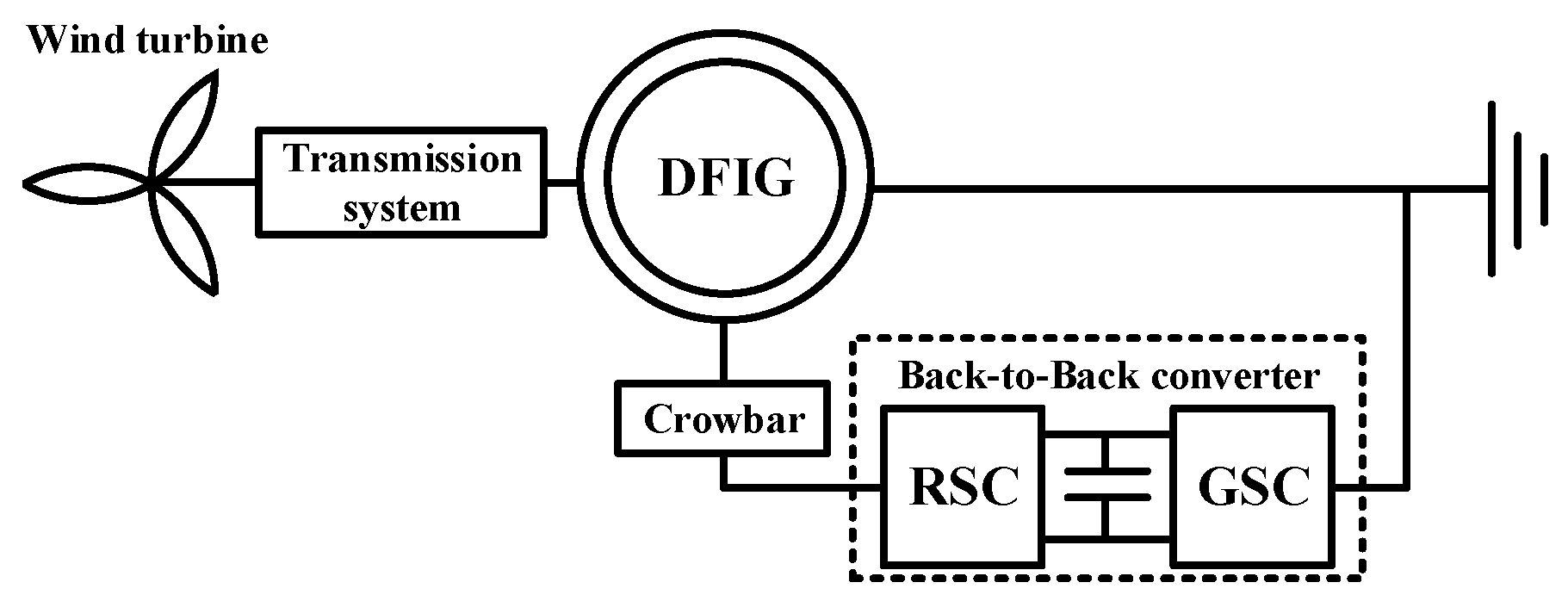
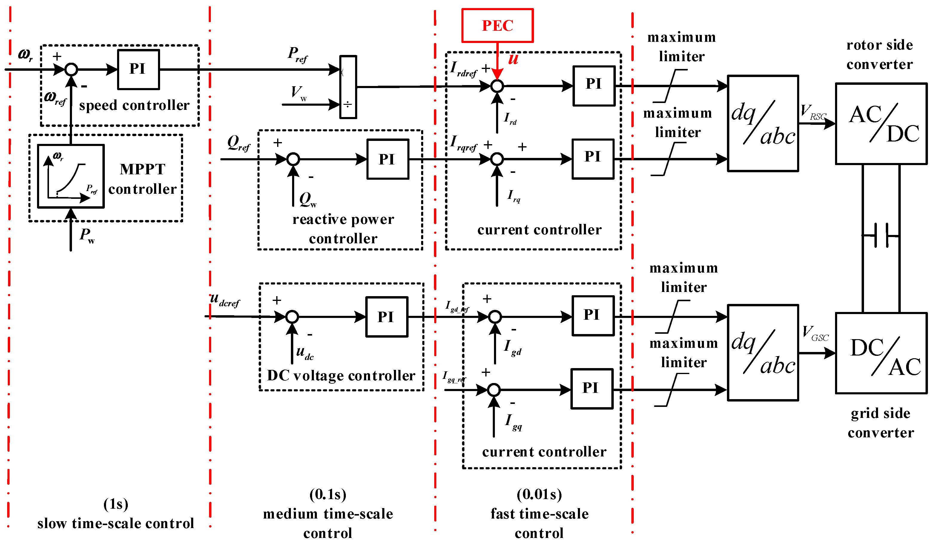
3.2. Controlled System Model
3.3. Design of PEC
4. Simulation Study
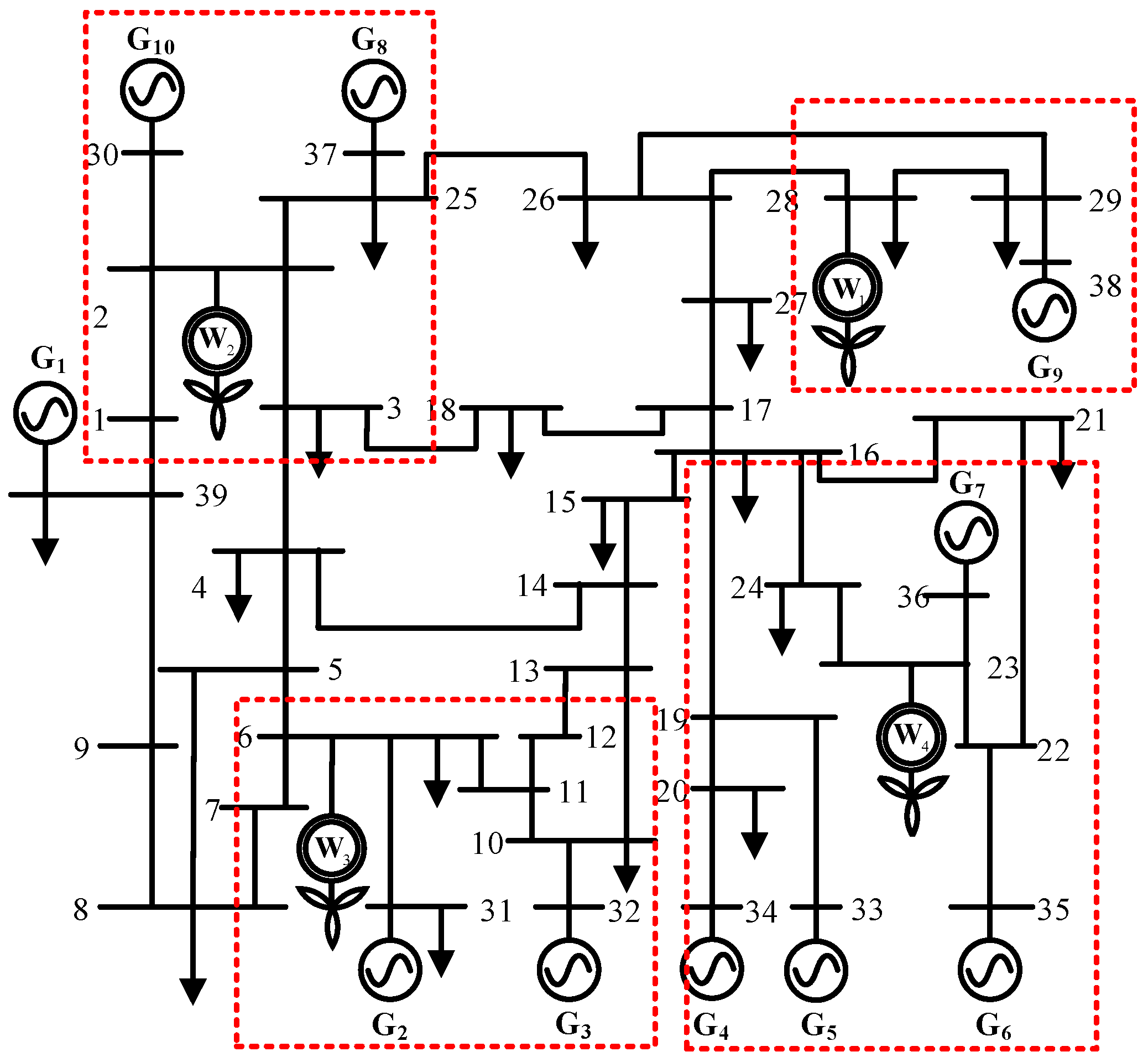
4.1. Test System
4.2. Configuration of PEC
4.3. General Performance of PEC
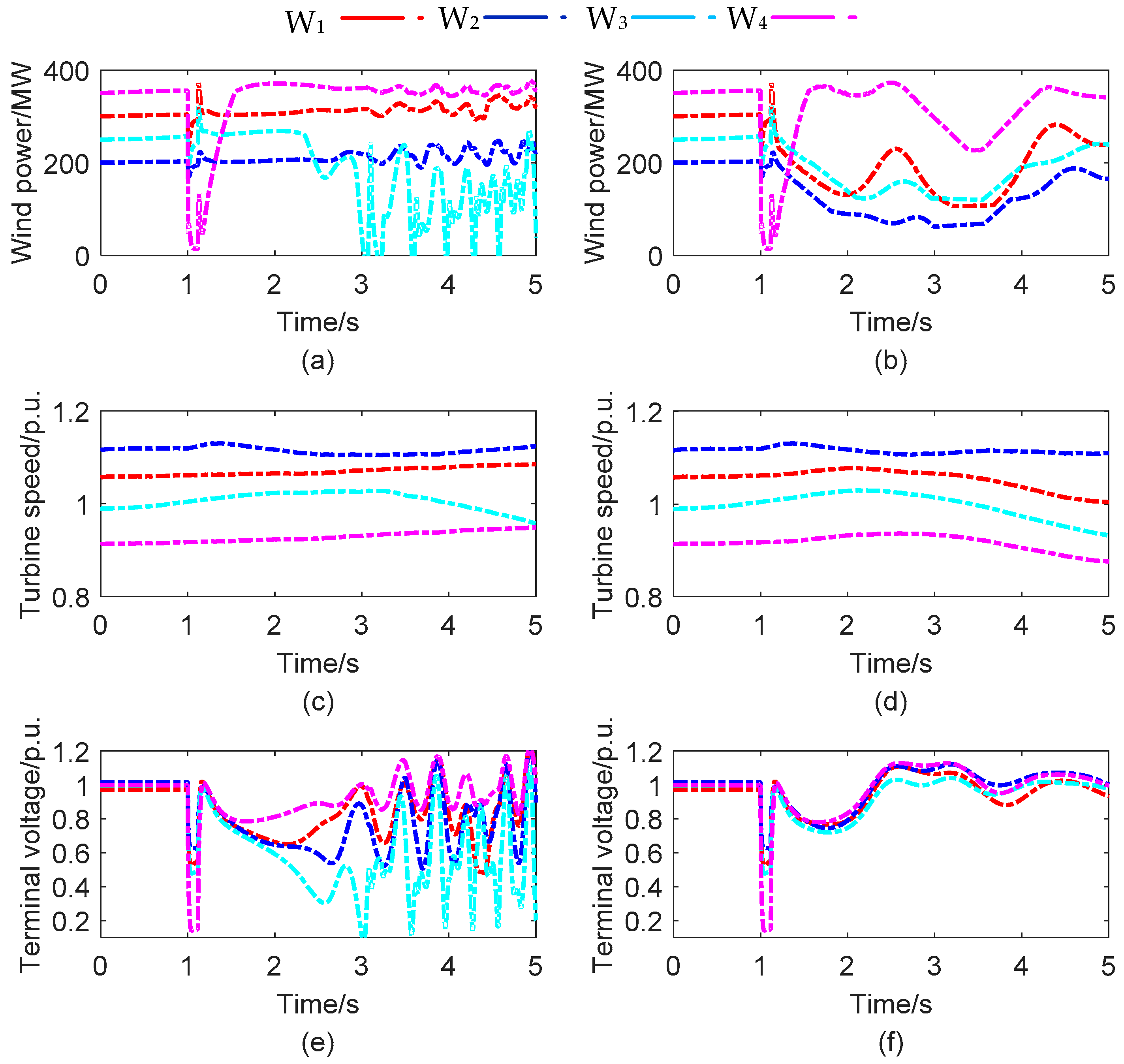
4.4. Robustness to Wind Speed Fluctuation
4.5. Robustness to the Communication Delay
5. Conclusions
Author Contributions
Funding
Conflicts of Interest
References
- Kundur, P. Power System Stability and Control; McGraw-Hill: New York, NY, USA, 1994. [Google Scholar]
- Wang, H.; Zhang, B.H.; Hao, Z.G. Response based emergency control system for power system transient stability. Energies 2015, 8, 13508–13520. [Google Scholar] [CrossRef]
- Xu, X.; Zhang, H.Z.; Li, C.G.; Liu, Y.T.; Li, W.; Terzija, V. Optimization of the event-driven emergency load-shedding considering transient security and stability constraints. IEEE Trans. Power Syst. 2017, 32, 2581–2592. [Google Scholar] [CrossRef]
- Zhang, Z.; Yang, H.; Yin, X.; Han, J.; Wang, Y.; Chen, G. A load-shedding model based on sensitivity analysis in on-line power system operation risk assessment. Energies 2017, 11, 727. [Google Scholar] [CrossRef]
- Zhou, Y.Z.; Huang, H.Y.; Xu, Z.; Hua, W.; Yang, F.Y.; Liu, S. Wide-area measurement system-based transient excitation boosting control to improve power system transient stability. IET Gener. Transm. Distrib. 2015, 9, 845–854. [Google Scholar] [CrossRef]
- Vittal, E.; O’Malley, M.; Keane, A. Rotor angle stability with high penetration of wind generation. IEEE Trans. Power Syst. 2012, 27, 353–362. [Google Scholar] [CrossRef]
- Edrah, M.; Lo, K.L.; Anaya-Lara, O. Impacts of high penetration of DFIG wind turbines on rotor angle stability of power systems. IEEE Trans. Sustain. Energy 2015, 6, 759–766. [Google Scholar] [CrossRef]
- Cardenas, R.; Pena, R.; Alepuz, S.; Asher, G. Overview of control systems for the operation of DFIGs in wind energy applications. IEEE Trans. Ind. Electron. 2013, 60, 2776–2798. [Google Scholar] [CrossRef]
- Liu, Z.Y.; Liu, C.R.; Li, G.Y.; Liu, Y.; Liu, Y.L. Impact study of PMSG-based wind power generation on power system transient stability using EEAC theory. Energies 2015, 8, 13419–13441. [Google Scholar] [CrossRef]
- Hossain, M.J.; Pota, H.R.; Mahmud, M.A.; Ramos, R.A. Investigation of the impacts of large-scale wind power penetration on the angle and voltage stability of power system. IEEE Syst. J. 2012, 6, 76–84. [Google Scholar] [CrossRef]
- Mitra, A.; Chatterjee, D. Active power control of DFIG-based wind farm for improvement of transient stability of power systems. IEEE Trans. Power Syst. 2016, 31, 82–93. [Google Scholar] [CrossRef]
- Werise, B. Impact of K-factor and active current reduction during fault-ride-through of generating units connected via voltage-sourced converters on power system stability. IET Renew. Power Gener. 2015, 9, 25–36. [Google Scholar]
- Ullah, N.R.; Thiringer, T.; Karlsson, D. Voltage and transient stability support by wind farms complying with the E.ON Netz grid code. IEEE Trans. Power Syst. 2007, 22, 1647–1656. [Google Scholar] [CrossRef]
- Eriksson, R. On the centralized nonlinear control of HVDC systems using Lyapunov Theory. IEEE Trans. Power Deliv. 2013, 28, 1156–1163. [Google Scholar] [CrossRef]
- Eriksson, R. Coordinated control of multiterminal DC grid power injections for improved rotor-angle stability based on Lyapunov theory. IEEE Trans. Power Deliv. 2014, 29, 1789–1797. [Google Scholar] [CrossRef]
- Mahmud, M.A.; Pota, H.R.; Aldeen, M.; Hossain, MJ. Partial feedback linearizing excitation controller for multimachine power systems to improve transient stability. IEEE Trans. Power Syst. 2014, 29, 561–571. [Google Scholar] [CrossRef]
- Lu, Q.; Sun, Y.Z. Nonlinear stabilizing control of multimachine systems. IEEE Trans. Power Syst. 1989, 4, 236–241. [Google Scholar] [CrossRef]
- Han, J.Q. From PID to active disturbance rejection control. IEEE Trans. Ind. Electron. 2009, 56, 900–906. [Google Scholar] [CrossRef]
- Hu, J.B.; Huang, Y.H.; Wang, D.; Yuan, H.; Yuan, X.M. Modeling of grid connected DFIG-based wind turbines for DC-link voltage stability analysis. IEEE Trans. Sustain. Energy 2015, 6, 1325–1336. [Google Scholar] [CrossRef]
- Ma, Y.; Liu, J.; Liu, H.; Zhao, S. Active-reactive additional damping control of a doubly-fed induction generator based on active disturbance rejection control. Energies 2018, 11, 1314. [Google Scholar] [CrossRef]
- Naduvathuparambil, B.; Valenti, M.C.; Feliachi, A. Communication delay in wide-area measurement systems. In Proceedings of the Thirty-Fourth Southeastern Symposium on System Theory (Cat. No.02EX540), Huntsville, AL, USA, 19 March 2002; pp. 118–122. [Google Scholar]


| Wind Farm | W1 | W2 | W3 | W4 |
|---|---|---|---|---|
| Wind speed | 8.62 m/s | 7.54 m/s | 8.12 m/s | 9.08 m/s |
| Active-power | 300 MW | 200 MW | 250 MW | 350 MW |
| Wind Condition | Fault | No Control | PEC | PEC with 100 ms Delay | PEC with 200 ms Delay |
|---|---|---|---|---|---|
| Constant | Line 15–16 | 112 ms | 136 ms | 130 ms | 128 ms |
| Line 2–3 | 130 ms | 172 ms | 168 ms | 166 ms | |
| Line 5–6 | 186 ms | 230 ms | 226 ms | 226 ms | |
| Variable (shown in Figure 9) | Line 15–16 | 106 ms | 132 ms | 128 ms | 126 ms |
| Line 2–3 | 123 ms | 168 ms | 164 ms | 164 ms | |
| Line 5–6 | 160 ms | 220 ms | 218 ms | 214 ms |
© 2018 by the authors. Licensee MDPI, Basel, Switzerland. This article is an open access article distributed under the terms and conditions of the Creative Commons Attribution (CC BY) license (http://creativecommons.org/licenses/by/4.0/).
Share and Cite
Shen, P.; Guan, L.; Huang, Z.; Wu, L.; Jiang, Z. Active-Current Control of Large-Scale Wind Turbines for Power System Transient Stability Improvement Based on Perturbation Estimation Approach. Energies 2018, 11, 1995. https://doi.org/10.3390/en11081995
Shen P, Guan L, Huang Z, Wu L, Jiang Z. Active-Current Control of Large-Scale Wind Turbines for Power System Transient Stability Improvement Based on Perturbation Estimation Approach. Energies. 2018; 11(8):1995. https://doi.org/10.3390/en11081995
Chicago/Turabian StyleShen, Peng, Lin Guan, Zhenlin Huang, Liang Wu, and Zetao Jiang. 2018. "Active-Current Control of Large-Scale Wind Turbines for Power System Transient Stability Improvement Based on Perturbation Estimation Approach" Energies 11, no. 8: 1995. https://doi.org/10.3390/en11081995