Efficient Forecasting of Electricity Spot Prices with Expert and LASSO Models

Abstract

Recent electricity price forecasting (EPF) studies suggest that the least absolute shrinkage and selection operator (LASSO) leads to well performing models that are generally better than those obtained from other variable selection schemes. By conducting an empirical study involving datasets from two major power markets (Nord Pool and PJM Interconnection), three expert models, two multi-parameter regression (called baseline) models and four variance stabilizing transformations combined with the seasonal component approach, we discuss the optimal way of implementing the LASSO. We show that using a complex baseline model with nearly 400 explanatory variables, a well chosen variance stabilizing transformation (asinh or N-PIT), and a procedure that recalibrates the LASSO regularization parameter once or twice a day indeed leads to significant accuracy gains compared to the typically considered EPF models. Moreover, by analyzing the structures of the best LASSO-estimated models, we identify the most important explanatory variables and thus provide guidelines to structuring better performing models.

1. Introduction

One of the challenges of short-term electricity price forecasting (EPF) is variable (or feature) selection. However, there is no standard approach when the number of potential explanatory variables is large. So far, the typical approach has been to select predictors in an ad-hoc fashion or by using expert knowledge [1]. Rarely has a formal validation procedure been carried out, and hardly ever has an automated selection or shrinkage algorithm been utilized.

The earliest known examples of statistically sound variable selection in EPF include Karakatsani and Bunn [2] and Misiorek [3] who used stepwise regression to eliminate statistically insignificant variables in parsimonious autoregression (AR) and regime-switching models in a multivariate setting, i.e., separately for the individual load periods; see [4] for a discussion of the uni- and multivariate frameworks in EPF. In the machine learning literature, Amjady and Keynia [5] proposed a feature selection algorithm based on mutual information that was later utilized in [6,7], among others. On the other hand, Gianfreda and Grossi [8] used a very simple technique—single-step elimination of insignificant predictors in a regression setting.

To our best knowledge, Barnes and Balda [9] were the first to apply regularization in EPF. Namely, in a study concerning the profitability of battery storage, they utilized ridge regression to compute forecasts of New York Independent System Operator (NYISO) electricity prices for a model with more than 50 regressors. By ‘putting big data analytics to work’—as they referred to it—Ludwig et al. [10] used random forests and the least absolute shrinkage and selection operator (LASSO or Lasso) as a feature selection algorithm to choose which of the 77 available weather stations were relevant. In parallel, in the machine learning literature, González et al. [11] utilized random forests, while Keles et al. [7] combined the k-Nearest-Neighbor algorithm with backward elimination to select the most appropriate inputs out of more than 50 fundamental parameters or lagged versions of these parameters.

The next qualitative change came with the papers by Ziel et al. [12,13], who used LASSO to sparsify very large (100+) sets of model parameters, either utilizing B-splines in a univariate setting or, more efficiently, within a multivariate framework. In the first thorough comparative study, Uniejewski et al. [14] evaluated six automated selection and shrinkage procedures (single-step elimination, forward and backward stepwise regression, ridge regression, LASSO, and elastic nets) applied to a baseline model with 100+ regressors. They concluded that using LASSO and elastic nets can bring significant accuracy gains compared to commonly used EPF models. Finally, in a study on the optimal model structure for short-term EPF, i.e., uni- vs. multivariate, Ziel and Weron [4] considered autoregressive models with 200+ potential explanatory variables (but not exogenous) and concluded that both uni- and multivariate LASSO-implied structures significantly outperform autoregressive benchmarks and that combining their forecasts can bring further improvements in predictive accuracy.

Yet, despite these very recent advances in the use of regularization techniques for EPF—and particularly the LASSO—a few issues remain open:

• Optimal structure of the baseline model. Which of the available regressors should we consider? Should the pool of regressors be parsimonious, limited mostly to lagged prices as in references [4,12,13,14]? Or the contrary, should we include as many regressors as possible, in particular, lagged exogenous variables?
• The choice of the LASSO tuning (or regularization) parameter $\lambda$. So far, two schemes have been proposed in the EPF literature. Ziel et al. [4,12,13] selected one $\lambda$ for each day and hour in the test period by maximizing an information criterion in the 730-day in-sample calibration window, while Uniejewski et al. [14] used one 91-day cross-validation window to select one $\lambda$ for all days and hours in the test period. Which approach leads to more accurate forecasts—frequent recalibration (every day and hour), one $\lambda$ for all days and hours, or something in between? What is the optimal window length for selecting $\lambda$?
• The use of variance stabilizing transformations (VSTs). Recent studies advocate utilizing the seasonal component approach of Nowotarski and Weron [15] to eliminate long-term trend-seasonal effects and applying a VST to ‘normalize’ the marginal price distributions prior to fitting a forecasting model. So far, only parsimonious regression and neural net structures have been tested. However, is this approach also beneficial in case of parameter-rich and LASSO-estimated models? If yes, which of the VSTs discussed and evaluated in Uniejewski et al. [16] are to be recommended?

To this end, we conduct a comprehensive empirical study involving nearly 5-year long datasets from two major power markets (Nord Pool and PJM Interconnection), multiple model structures (including three expert models, two multi-parameter regression baseline models and LASSO-estimated models based on the latter two structures), a range of alternative procedures for estimating $\lambda$, four variance stabilizing transformations combined with the seasonal component approach, and an evaluation in terms of the classical error measure for point forecasts (i.e., the mean absolute error, MAE) and the Diebold–Mariano (DM) test [17] to determine significant differences in forecasting accuracy.

For the benchmarks, we consider a naive similar-day scheme and three parsimonious autoregressive models with exogenous variables (ARX). Two of them are built on popular structures, originally proposed by Misiorek et al. [18] and Ziel and Weron [4], and the third one is a new specification that was motivated by the results presented in Table 2 of Uniejewski et al. [14]. Following the later paper and Ziel [13], we refer to all three ARX benchmarks as expert models, since they are built on some prior knowledge of experts. As the baseline structures that are ‘shrunk’ via LASSO, we use two multi-parameter ARX models—one has been already considered in the EPF context [14], and the other is a newly proposed specification. Furthermore, we propose a new two-step procedure that merges automated variable selection via LASSO with ordinary least squares (OLS) estimation of its weights and compare the obtained point forecasts across four variance stabilizing transformations (VSTs) and 39 schemes of selecting the tuning parameter ($\lambda$).

The remainder of the paper is structured as follows. In Section 2, we first introduce the two datasets and the rolling window scheme, and then discuss seasonal decomposition and the four VSTs used in this study. In Section 3, we introduce the considered model structures. Then, in Section 4, we compare the predictive performance in terms of MAE and the DM test across models, VSTs, and $\lambda$-selection schemes. We also analyze the structures of the best LASSO-estimated models to identify the most important explanatory variables and thus provide guidelines to structuring better performing models. Finally, in Section 5, we wrap up the results and conclude.

2. Methodology

2.1. The Test Ground

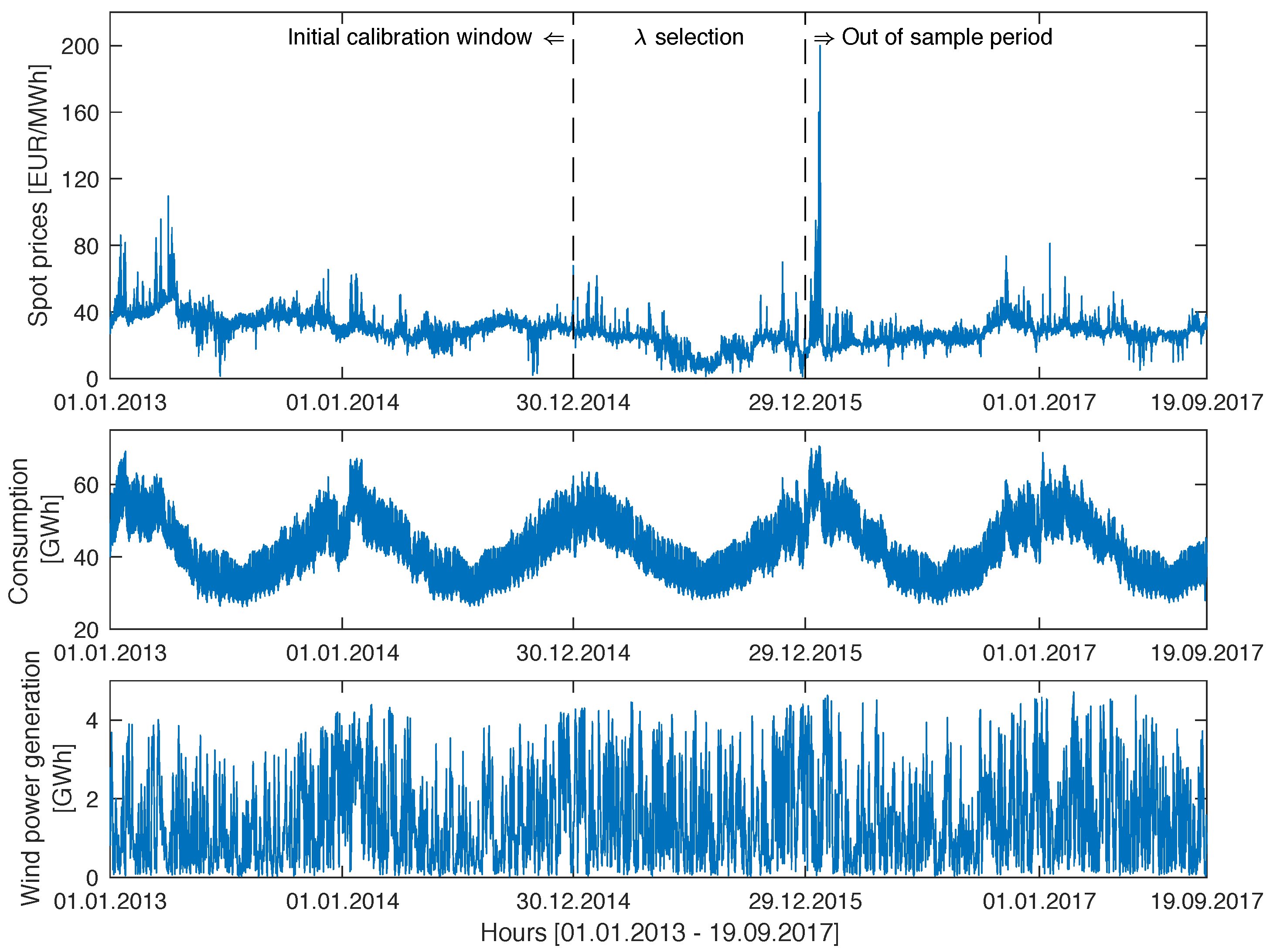
For the test ground we chose two major power markets—Nord Pool (Europe) and PJM (United States). The first dataset comprises system prices, day-ahead consumption prognosis for four Nordic countries (Denmark, Finland, Norway, and Sweden), and day-ahead wind power generation prognosis for the period 1 January 2013 to 19 September 2017, all at hourly resolution. The time series plotted in Figure 1 were constructed using data published by the Nordic power exchange Nord Pool (www.nordpoolspot.com) and preprocessed to account for missing values and changes to/from daylight saving time, analogously as in [19]. The missing data values (corresponding to the changes to the daylight saving/summer time and eight hourly consumption figures for Norway) were substituted by the arithmetic average of the neighboring values. The ‘doubled’ values (corresponding to the changes from the daylight saving/summer time) were substituted by the arithmetic average of the two values for the ‘doubled’ hour.

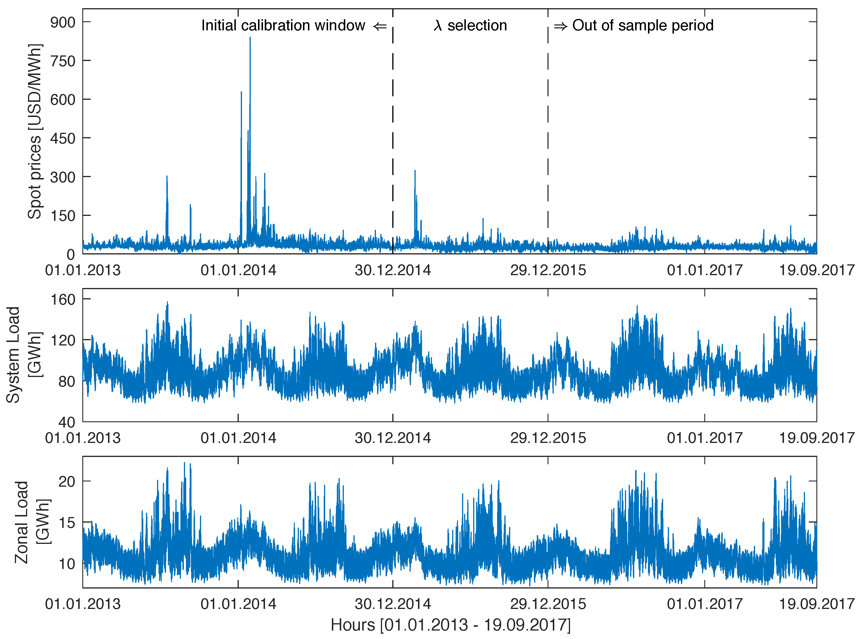
The second dataset comprises hourly prices for the Commonwealth Edison (COMED) zone in the PJM market and day-ahead system (RTO) and zonal (COMED) load forecasts for the same period, i.e.,1 January 2013 to 19 September 2017 (see Figure 2). The time series were constructed using data published by the PJM (www.pjm.com) and preprocessed to account for missing values and changes to or from the daylight saving time, analogously, as for the Nord Pool dataset. Note, that although the electricity price units are similar in Figure 1 and Figure 2 (EUR/MWh vs. USD/MWh), the scales on the y-axis are different because of the much more volatile behavior of the PJM market, particularly in 2014.

Like the majority of EPF studies, we considered a rolling window scheme. To avoid seasonal artifacts, we let the calibration window length be a multiple of the weekly and annual periodicities. On the other hand, due to a large number of variables considered (as many as 386 in one of the models), we needed a window of more than 386 days to avoid an underdetermined system with fewer equations than unknowns. Hence, the choice of a circa two-year calibration window of 728 days or 104 full weeks which is the shortest window that satisfies the these criteria.

Each day, the 728-day long calibration window was rolled forward by 24 h and price forecasts for the 24 h of the next day were computed. Initially, all considered models (their short-term and long-term components) were calibrated with data from 1 January 2013 to 19 September 2017 and forecasts for all 24 h of 30 December 2014 were determined. Then, the window was rolled forward by one day and forecasts for all 24 h of the next day are computed. This procedure is repeated until predictions for the last day in the sample (i.e., 19 September 2017) were made.

2.2. Seasonal Decomposition

Recent published research leaves no doubt that seasonal decomposition of the price series leads to significant improvement in forecasting accuracy [15,20,21]. Here, we followed the Seasonal Component AutoRegressive (SCAR) modeling framework of Nowotarski and Weron [15], i.e., the series of electricity spot prices is decomposed in an additive manner into a long-term seasonal component (LTSC) and the remaining stochastic component with short-term periodicities. Then, the two were modeled separately and their day-ahead forecasts are added up to yield the final price forecast. Note that following Uniejewski et al. [21], we added an additional step to the original SCAR algorithm, in which we decomposed the exogenous series (consumption prognosis and wind power generation prognosis; see Section 2.1).

Moreover, in contrast to other papers built around the seasonal component concept, (i) we did not limit the analysis to log-transformed data but considered more general variance stabilizing transformations (see Section 2.3) and (ii) worked only with the S${}_9$ wavelet-based LTSC [19,22] which has been found to be robust and well performing across a range of datasets and forecasting models [20,21].

2.3. Variance Stabilizing Transformations

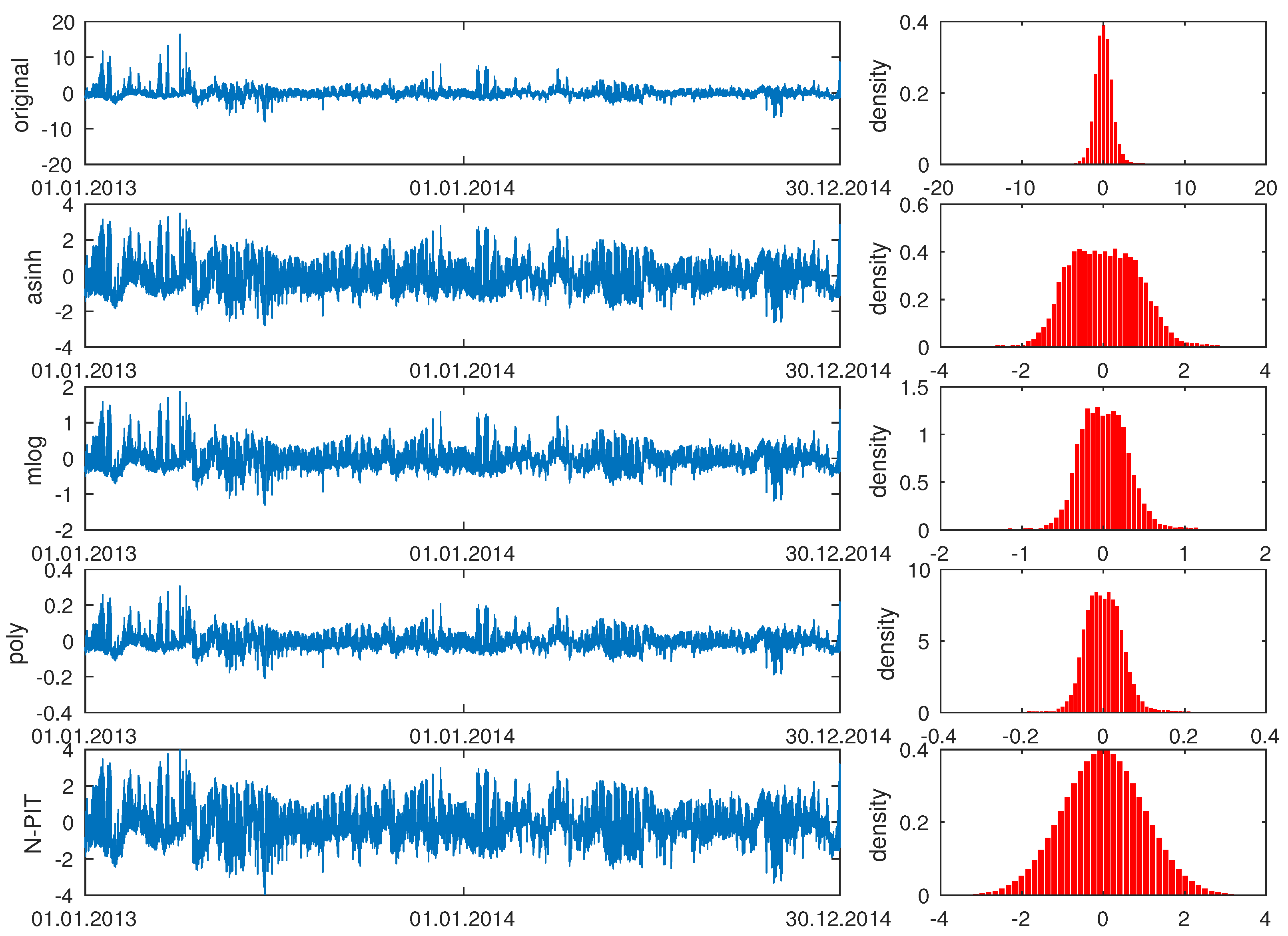
The basic idea behind a variance stabilizing transformation (VST) is to reduce the variation in price data. Lower variation and/or less spiky behavior of the input data usually allows the forecasting model to yield more accurate predictions [22]. In our models, we let $Y_{d,h}$ denote the deseasonalized electricity price in the day-ahead market for day d and hour h, with $X_{d,h}$ being transformed data, i.e., $X_{d,h}=f\left(Y_{d,h}\right)$, where $f(·)$ is a given VST. After computing the forecasts, we applied the inverse transformation to obtain the deseasonalized electricity spot price forecasts: ${\widehat{Y}}_{d,h}=f^{-1}({\widehat{X}}_{d,h})$. We used four VST classes that have been found to perform well in an EPF context [16]. Three of them work on ‘normalized’ values, $y_{d,h}=\frac{1}{b}(Y_{d,h}-a)$, where a is the median of $Y_{d,h}$ in the 728-day calibration window and b is the sample median absolute deviation (MAD) around the median. The last class builds on the probability integral transform (PIT) and does not require normalization. In Figure 3, we illustrate all four VSTs on a sample dataset.

The area hyperbolic sine transformation is nothing else but the inverse of the hyperbolic sine,

$$X_{d,h}=\mathbf{asinh}\left(y_{d,h}\right)\equiv \log \left(y_{d,h}+\sqrt{y_{d,h}^2+1}\right),$$

(1)

with inverse $y_{d,h}=\sin \mathrm{h}\left(X_{d,h}\right)$. It has been used in the context of electricity prices, e.g., by Schneider [23] and Ziel and Weron [4]. The mirror-log and polynomial transformations were introduced by Uniejewski et al. [16] as generalizations of the robust Box–Cox transformation for $\lambda =0$ and $\lambda \ne 0$, respectively. The former is a straightforward generalization of the log-transformation with a mirror image of the logarithm for negative values:

$$\begin{array}{c}\hfill X_{d,h}=\mathbf{mlog}(y_{d,h},c)=\mathrm{sgn}\left(y_{d,h}\right)\left[\log \left(|y_{d,h}|+\frac{1}{c}\right)+\log \left(c\right)\right],\end{array}$$

(2)

with inverse $y_{d,h}=\mathrm{sgn}\left(X_{d,h}\right)\left[e^{|X_{d,h}|-\log c}-\frac{1}{c}\right].$ It is a one parameter family. Here, we used $c=\frac{1}{3}$, as suggested by Uniejewski et al. [16]. Similarly to the standard log-transformation and asinh, the mlog exhibits a log-damping effect. The used polynomial transformation was

$$\begin{array}{c}\hfill X_{d,h}=\mathbf{poly}(y_{d,h},c,\lambda )=\mathrm{sgn}\left(y_{d,h}\right)\left[{\left||y_{d,h}|+{\left(\frac{c}{\lambda }\right)}^{\frac{1}{\lambda -1}}\right|}^{\lambda }-{\left(\frac{c}{\lambda }\right)}^{\frac{\lambda }{\lambda -1}}\right],\end{array}$$

(3)

with inverse $y_{d,h}=\mathrm{sgn}\left(X_{d,h}\right)[\{|X_{d,h}|+{\left(\frac{c}{\lambda }\right)}^{\frac{\lambda }{\lambda -1}}{\}}^{\frac{1}{\lambda }}-{\left(\frac{c}{\lambda }\right)}^{\frac{1}{\lambda -1}}]$. It is a two parameter family. Here, we used $\lambda =0.125$ and $c=0.05$, as suggested by Uniejewski et al. [16]. Both the mlog and poly had slopes of c at the origin.

The last class we considered is based on the so-called probability integral transform: $\mathrm{PIT}\left(Z\right)=F_Z\left(Z\right)$, where $F_Z$ is the cumulative distribution function (cdf) of Z. The N-PIT is defined as

$$X_{d,h}=\mathbf{N}\text{-}\mathbf{PIT}\left(Y_{d,h}\right)\equiv {\mathrm{\Phi }}^{-1}\left(\mathrm{PIT}\left(Y_{d,h}\right)\right)={\mathrm{\Phi }}^{-1}\left({\widehat{F}}_Y\left(Y_{d,h}\right)\right),$$

(4)

with the inverse $Y_{d,h}={\widehat{F}}_Y^{-1}\left(\mathrm{\Phi }\left(X_{d,h}\right)\right)$, where $\mathrm{\Phi }$ is the standard normal cdf. The N-PIT, misleadingly called the Nataf transformation, was used by Diaz and Planas [24] to normalize Spanish electricity prices. It was also used together with the t-PIT (a Student-t transformed PIT) in a recent extensive EPF study [16]. In Figure 3, we can clearly see that the histogram of N-PIT-transformed prices looks like the standard normal density.

2.4. The Forecasting Framework

Let us now summarize the forecasting framework. For each autoregressive model discussed in Section 3, i.e., all models except the naive benchmark, this consisted of five steps:

• (a)

  Decompose the series of prices in the calibration window of $728\times 24=17,472$ h using S${}_9$ wavelet smoothing, i.e., utilizing nine decomposition levels [19,22], into a trend-seasonal and a stochastic component (with short-term periodicities): $P_{d,h}=T_{d,h}+Y_{d,h}$.

  (b)

  Compute persistent forecasts of the LTSC independently for each of the 24 h of the next day, i.e., ${\widehat{T}}_{d^{*}+1,h}\equiv T_{d^{*},h}$ for $h=1,\dots ,24$, where $d^{*}$ is the last day in the calibration window.

  (c)

  Decompose the exogenous series in the calibration window of $(728+1)\times 24=17,496$ h using the same type of wavelet smoothing as in Step 1(a). Note that we can start one day earlier since the load and wind power forecasts are known one day in advance.

• Normalize $y_{d,h}=\frac{1}{b}(Y_{d,h}-a)$ and transform $X_{d,h}=f\left(y_{d,h}\right)$, the stochastic component, where f is one of the VSTs defined in Section 2.3 and $(a,b)=$ (median, MAD) of $Y_{d,h}$ in the calibration window. Analogously normalize and transform the stochastic component(s) of the exogenous series.
• Calibrate one of the autoregressive models discussed in Section 3 to $X_{d,h}$ and compute forecasts for each hour of the next day: ${\widehat{X}}_{d^{*}+1,h},h=1,\dots ,24$.
• Back-transform the obtained forecasts: ${\widehat{Y}}_{d^{*}+1,h}=b{f}^{-1}\left({\widehat{X}}_{d^{*}+1,h}\right)+a$.
• Add the persistent LTSC forecasts to yield the final price forecasts: ${\widehat{P}}_{d^{*}+1,h}={\widehat{T}}_{d^{*}+1,h}+{\widehat{Y}}_{d^{*}+1,h}$.

Note that compared to recent EPF papers utilizing the seasonal component approach [15,20,21], we introduced important changes. Firstly, instead of the logarithm we used one of four VSTs defined in Section 2.3, which can also be applied to price series with negative values, like those from the German European Energy Exchange (EEX) [25]. Secondly, the order of data transformation and decomposition was swapped. We first seasonally decomposed the data, and then transformed the stochastic part; the same applied for the exogenous series (consumption and wind power generation prognosis).

3. Models

3.1. Benchmarks

The first benchmark, the so-called naive method, belongs to the class of similar-day techniques. It is defined by ${\widehat{P}}_{d,h}=P_{d-7,h}$ for Monday, Saturday and Sunday, and ${\widehat{P}}_{d,h}=P_{d-1,h}$ otherwise. As Contreras et al. [26] argued, forecasting procedures that are not calibrated carefully fail to outperform this extremely simple method surprisingly often.

The second benchmark, denoted by ARX1, is a simple autoregressive structure originally proposed by Misiorek et al. [18] and later used in a number of EPF studies [13,14,19,20,27,28,29,30]:

$$\begin{array}{cc}\hfill X_{d,h}=& {\beta }_{h,1}{X}_{d-1,h}+{\beta }_{h,2}{X}_{d-2,h}+{\beta }_{h,3}{X}_{d-7,h}+{\beta }_{h,4}{X}_{d-1}^{min}+{\beta }_{h,5}{C}_{d,h}\hfill \\ & +{\beta }_{h,6}{D}_{Sat}+{\beta }_{h,7}{D}_{Sun}+{\beta }_{h,8}{D}_{Mon}+{\epsilon }_{d,h},\hfill \end{array}$$

(5)

where $X_{d-1,h}$, $X_{d-2,h}$ and $X_{d-7,h}$ refer to the transformed and deseasonalized price series. They account for the autoregressive effects of the previous days (the same hour yesterday, two days ago, and one week ago), while $X_{d-1}^{min}$ is the minimum of the previous day’s 24 hourly preprocessed prices. The exogenous variable $C_{d,h}$ refers to the prognosis of consumption for day d and hour h (actually, to a transformed and deseasonalized series). The three dummy variables $D_{Sat}$, $D_{Sun}$ and $D_{Mon}$ account for the weekly seasonality, and are defined as $D_i=1$ for $d=i$ and zero otherwise. Finally, the ${\epsilon }_{d,h}$s are assumed to be independent and identically distributed normal variables.

The third benchmark was the $exper{t}_{DoW,nl}$ model of Ziel and Weron [4], only expanded to include one exogenous variable (consumption prognosis). The model, denoted by ARX2, is given by the following formula:

$$\begin{array}{cc}\hfill X_{d,h}=& {\beta }_{h,1}{X}_{d-1,h}+{\beta }_{h,2}{X}_{d-2,h}+{\beta }_{h,3}{X}_{d-7,h}+{\beta }_{h,4}{X}_{d-1,24}\hfill \\ & +{\beta }_{h,5}{X}_{d-1}^{min}+{\beta }_{h,6}{X}_{d-1}^{max}+{\beta }_{h,7}{C}_{d,h}+\sum _{i=1}^7{\beta }_{h,8,i}{D}_i+{\epsilon }_{d,h}.\hfill \end{array}$$

(6)

The price for the last load period of the previous day, i.e., $X_{d-1,24}$, is included to take advantage of the fact that prices for early morning hours depend more on the previous day’s price at midnight than on the price for the same hour [13,31]. Compared to ARX1, the maximum of the previous day’s prices, i.e., $X_{d-1}^{max}$, and dummies for the remaining days of the week ($D_4\equiv D_{Tue},$$D_5\equiv D_{Wed},D_6\equiv D_{Thu},D_7\equiv D_{Fri}$) are also included. As there are seven dummies in Equation (6), one of them plays the role of the intercept. Note, that there is no intercept in Equation (5); this is not a major shortcoming since the prices are deseasonalized (i.e., centered) beforehand.

The last benchmark, denoted by ARX3, is based on the results of Uniejewski et al. [14]. The authors used shrinkage methods (particularly, LASSO and elastic nets) to find the most commonly selected regressors of a multi-variable ARX model. We analyzed these results and used them to construct a benchmark model that combines the knowledge of experts and the outcome of automated variable selection. The model is defined by

$$\begin{array}{cc}\hfill X_{d,h}=& {\beta }_{h,1}{X}_{d-1,h}+{\beta }_{h,2}{X}_{d-7,h}+{\beta }_{h,3}{X}_{d-1,h-1}+{\beta }_{h,4}{X}_{d-1,h+1}\hfill \\ & +{\beta }_{h,5}{X}_{d-1,21}+{\beta }_{h,6}{X}_{d-1,22}+{\beta }_{h,7}{X}_{d-1,24}+{\beta }_{h,8}{X}_{d-2,24}\hfill \\ & +{\beta }_{h,9}{C}_{d,h}+{\beta }_{h,10}{C}_{d-7,h}+{\beta }_{h,11}{W}_{d,h}+\sum _{i=1}^7{\beta }_{h,12,i}{D}_i+{\epsilon }_{d,h}.\hfill \end{array}$$

(7)

Compared to ARX2, this benchmark includes more autoregressive terms and two additional exogenous variables: consumption prognosis for the previous week, i.e., $C_{d-7,h}$, and wind power generation prognosis (for Nord Pool) or zonal load forecast (for PJM) of the forecasted day and hour, i.e., $W_{d,h}$. Actually, the latter two refer to transformed and deseasonalized values.

3.2. Baseline Autoregressive Models

An indisputable advantage of using automatic variable selection is an almost unlimited number of initially considered explanatory variables. As a result, the knowledge of experts becomes less important. However, the human factor is not completely eliminated. The forecaster still has to choose an appropriate baseline model that includes all variables of (potential) interest. To see how much this choice impacts the forecasting accuracy, we considered two different baseline models. The first one, denoted by bARX1, is essentially the fARX model of Uniejewski et al. [14] with consumption prognosis $C_{d,h}$ as the first exogenous variable and wind power generation prognosis (for Nord Pool) or zonal load forecast (for PJM) $W_{d,h}$ as the second, both after decomposition and transformation:

$$\begin{array}{cc}\hfill X_{d,h}=& \sum _{i=1}^3\sum _{j=1}^{24}{\beta }_{h,i,j,1}{X}_{d-i,j}+{\beta }_{h,7,h,1}{X}_{d-7,h}\hfill \\ & +\sum _{i=1}^3\left({\beta }_{h,i,1,2}{X}_{d-i}^{min}+{\beta }_{h,i,1,3}{X}_{d-i}^{max}\right)\hfill \\ & +{\beta }_{h,0,h,4}{C}_{d,h}+{\beta }_{h,1,h,4}{C}_{d-1,h}+{\beta }_{h,7,h,4}{C}_{d-7,h}+{\beta }_{h,0,h,5}{W}_{d,j}\hfill \\ & +\sum _{i=1}^7{\beta }_{h,i,1,6}{D}_i+\sum _{i=1}^7{\beta }_{h,i,1,7}{D}_i{X}_{d-1,h}+\sum _{i=1}^7{\beta }_{h,i,1,8}{D}_i{C}_{d,h}+{\epsilon }_{d,h}.\hfill \end{array}$$

(8)

Note that in contrast to the benchmark autoregressive models discussed in Section 3.1, we treated holidays as the eighth day of the week, i.e., $D_1=\dots =D_7=0$ for national holidays in Norway (for Nord Pool) or in the United States (for PJM); they were identified using the Time and Date AS web page: www.timeanddate.com/holidays. Consequently, like the ARX1 model, but unlike ARX2 and ARX3, the regression in Equation (8) has no intercept.

The second baseline model, denoted by bARX2, is much richer (386 vs. 104 variables). It uses information about prices from all hours of the whole previous week, the exogenous variables play much more important roles (175 vs. 4 variables) and the part accounting for weekly seasonality is more complex (the dummies are additionally multiplied by the average price from the previous day and the last known spot price, transformed, and deseasonalized). The model is given by

$$\begin{array}{cc}\hfill X_{d,h}=& \sum _{i=1}^7\sum _{j=1}^{24}{\beta }_{h,i,j,1}{X}_{d-i,j}+\sum _{i=1}^7\left({\beta }_{h,i,1,2}{X}_{d-i}^{min}+{\beta }_{h,i,1,3}{X}_{d-i}^{max}\right)\hfill \\ & +\sum _{i=\{0,1,2,7\}}\sum _{j=1}^{24}{\beta }_{h,i,j,4}{C}_{d-i,j}+\sum _{i=\{0,1,7\}}\sum _{j=1}^{24}{\beta }_{h,i,j,5}{W}_{d-i,j}\hfill \\ & +\sum _{i=1}^8{\beta }_{h,i,1,6}{D}_i+\sum _{i=1}^7{\beta }_{h,i,1,7}{D}_i{X}_{d-1,h}+\sum _{i=1}^7{\beta }_{h,i,1,8}{D}_i{X}_{d-1,24}\hfill \\ & +\sum _{i=1}^7{\beta }_{h,i,1,9}{D}_i{X}_{d-1}^{avg}+\sum _{i=1}^7{\beta }_{h,i,1,10}{D}_i{C}_{d,h}+{\epsilon }_{d,h}.\hfill \end{array}$$

(9)

Note that for $h=24$, ${\beta }_{h,i,1,8}\equiv 0$ for all i. Moreover, compared to bARX1, the model includes an explicit holiday dummy variable ($D_8$); hence, the regression in Equation (9) includes an intercept.

3.3. LASSO-Estimated Models

Let us write the structure of both baseline models in a more compact form:

$$X_{d,h}=\sum _{i=1}^n{\beta }_{h,i}{V}_{d,h}^i,$$

(10)

where the $V_{d,h}^i$s are the regressors, and the ${\beta }_{h,i}$s are the corresponding coefficients. Shrinkage (also known as regularization) fits the full model with all predictors using an algorithm that shrinks the coefficients of the less important explanatory variables towards zero [32]. The least absolute shrinkage and selection operator (LASSO or Lasso) of Tibshirani [33] may actually shrink some of the coefficients to zero and hence perform variable selection.

The LASSO can be treated as a generalization of linear regression, where instead of minimizing only the residual sum of squares (RSS), the sum of RSS and a linear penalty function of the $\beta$s is minimized:

$${\widehat{\mathit{\beta }}}_h^L=\underset{\mathit{\beta }}{min}\left\{\mathrm{RSS}+\lambda \parallel {\mathit{\beta }}_h{\parallel }_1\right\}=\underset{\mathit{\beta }}{min}\left\{\mathrm{RSS}+\lambda \sum _{i=1}^n|{\beta }_{h,i}|\right\},$$

(11)

where $\lambda \ge 0$ is a tuning (or regularization) parameter. Note that for $\lambda =0$, we get the standard least squares estimator, for $\lambda \to \infty$, all ${\beta }_{h,i}$s tend to zero, while for intermediate values of $\lambda$, there is a balance between minimizing the RSS and shrinking the coefficients towards zero (and each other). Selecting a ‘good’ value for $\lambda$ is critical. However, to our best knowledge, the optimal choice of $\lambda$ has not been discussed in the EPF context so far. We compared alternative $\lambda$-selection schemes for a grid of 25 exponentially decreasing $\lambda$s ranging from ${10}^0$ to ${10}^{-6}$, and selected the tuning parameter for which the mean absolute (prediction) error in the D-day validation period was the smallest.

Models for which the LASSO operator is used to estimate parameters are denoted by $\ast {\mathbf{Lasso}}_i^D$, where $i=1,2$ refers to one of two baseline models (respectively bARX1 and bARX2); D is the length of the validation window; and the asterisk represents the $\lambda$-selection scheme. We considered eight window lengths—$D=1$ (one day), 7 (one week), 28 (one ‘month’), 60 (two months), 91 (one quarter), 182 (half a year), 273 (three quarters) and 364 (one year)—and six $\lambda$-selection schemes:

• 24xN${\mathbf{Lasso}}_i^D$, where for each day and each hour in the test period, one $\lambda$ is selected,
• 2xN${\mathbf{Lasso}}_i^D$, where for each day in the test period, two $\lambda$s are selected—one for the on-peak and one for the off-peak hours,
• 1xN${\mathbf{Lasso}}_i^D$, where for each day in the test period, one $\lambda$ is selected,
• 24${\mathbf{Lasso}}_i^D$, where for each hour, one $\lambda$ is selected for the whole test period,
• 2${\mathbf{Lasso}}_i^D$, where two $\lambda$s are selected (on-peak and off-peak) for the whole test period,
• 1${\mathbf{Lasso}}_i^D$, where one $\lambda$ is selected for the whole test period.

3.4. LassOLS-Type Models

To answer the question of how important the shrinkage property is for reducing the prediction errors, we introduced a modification of the $\ast {\mathbf{Lasso}}_i^D$ class of models, where the LASSO operator is used to select the explanatory variables but not to estimate the ${\mathit{\beta }}_h$s; instead, we used OLS to obtain parameter estimates for the LASSO-selected variables. In this way, we automatically created 24 different ‘expert’, LASSO-implied models for each day. Since these model structures are dependent on the choice of $\lambda$, like in Section 3.3, we considered six model schemes: nxN${\mathbf{LassOLS}}_i^D$ and $n{\mathbf{LassOLS}}_i^D$, with $n=1,2,24$, which correspond to nxN${\mathbf{Lasso}}_i^D$ and $n{\mathbf{Lasso}}_i^D$ models, respectively.

4. Empirical Results

4.1. Evaluation in Terms of MAE and the DM Test

As the main evaluation criterion, we considered the mean absolute error (MAE) for the full out-of-sample test period of $D=631$ days, i.e., 29 December 2015 to 19 September 2017:

$$\mathrm{MAE}=\parallel {\mathcal{E}}_{d,h}{\parallel }_1=\frac{1}{24D}\sum _{d=1}^D\sum _{h=1}^{24}|{\mathcal{E}}_{d,h}|,$$

(12)

where ${\mathcal{E}}_{d,h}=P_{d,h}-{\widehat{P}}_{d,h}$ is the prediction error for a given day d and hour h. Additionally, we used the Diebold–Mariano (DM) test [17] to draw statistically significant conclusions on the outperformance of the forecasts of one model by those of another. In the EPF literature, the DM test is usually performed separately for each hour of the day [1]. However, Ziel and Weron [4] recently introduced a different approach, where only one statistic for each pair of models is computed based on the 24-dimensional vector of errors for each day:

$${\Delta }_{X,Y,d}=\parallel {\mathcal{E}}_{X,d}\parallel -\parallel {\mathcal{E}}_{Y,d}\parallel ,$$

(13)

where $\parallel {\mathcal{E}}_{Z,d}\parallel ={\sum }_{h=1}^{24}|{\mathcal{E}}_{d,h}|$ for model Z. For each model pair and each dataset, we computed the p-value of two one-sided DM tests: (i) a test with the null hypothesis $H_0:E\left({\Delta }_{X,Y,d}\right)\le 0$, i.e., the outperformance of the forecasts of Y by those of X, and (ii) the complementary test with the reverse null $H_0^R:E\left({\Delta }_{X,Y,d}\right)\ge 0$, i.e., the outperformance of the forecasts of X by those of Y. As in the standard DM test, we assumed that the loss differential series was covariance stationary.

4.2. Performance across Model Classes and VSTs

In

Table 1. Mean absolute errors (MAE) in the 631-day test period for 30 considered models (in rows), five variance stabilizing transformations (VSTs; in columns; the first ‘transformation’ is identity, Id) and two markets (Nord Pool and PJM). The models include four benchmarks, two baseline models, 12 $\ast {\mathbf{LassOLS}}_i^{91}$ models and 12 $\ast {\mathbf{Lasso}}_i^{91}$ models. Note that all LASSO-type models use a 91-day validation window for selecting $\lambda$. 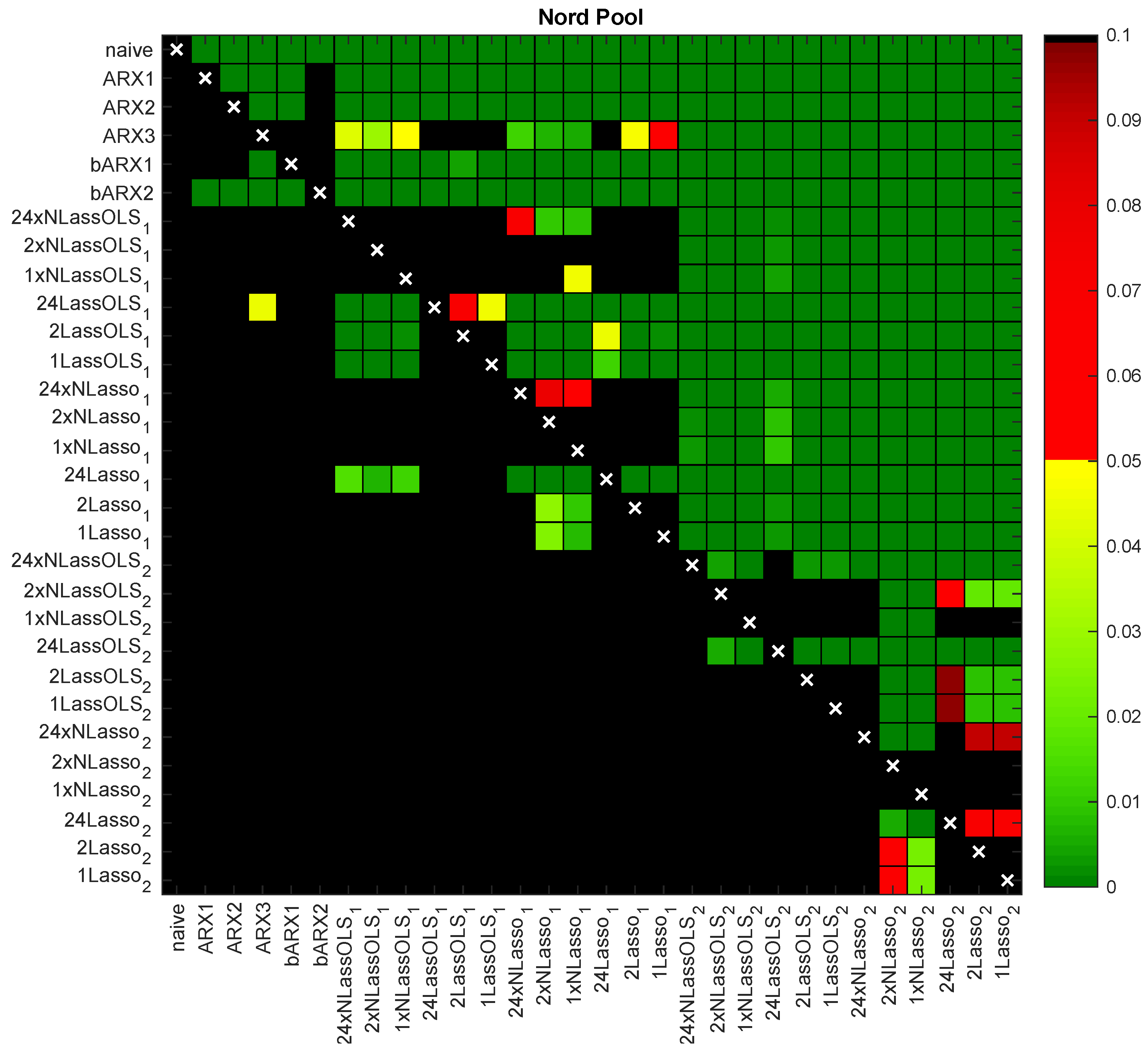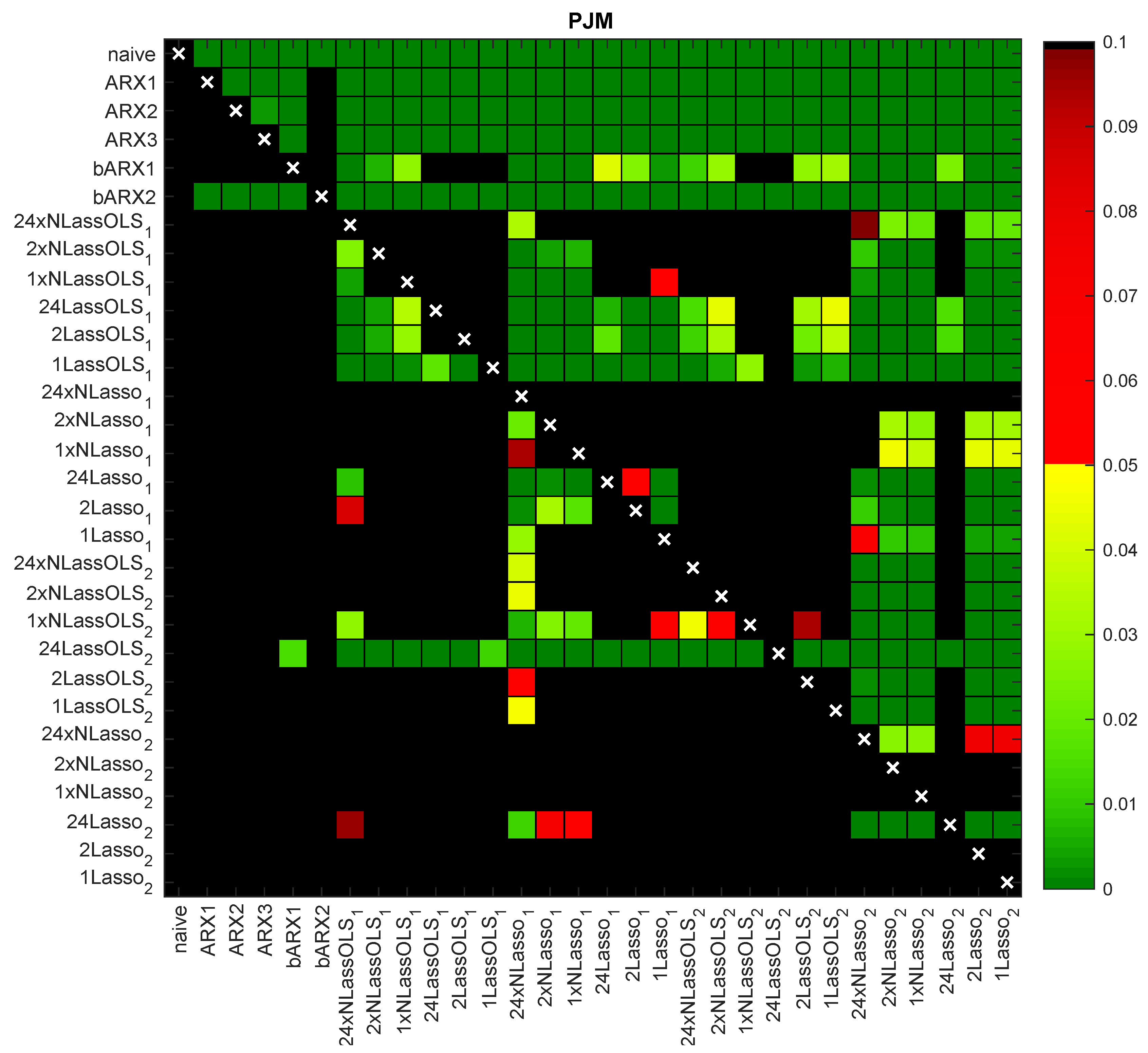A heat map is used to indicate better (→green) and worse (→red) results.

, we report the MAEs in the 631-day test period for 30 considered models and five VSTs (Id denotes the identity ‘transformation’). The models include four benchmarks, two baseline models, 12 $\ast {\mathbf{LassOLS}}_i^{91}$ models and 12 $\ast {\mathbf{Lasso}}_i^{91}$ models, i.e., LASSO-type models with a 91-day validation window to select $\lambda$. In Figure 4 and Figure 5, the results of the ‘multivariate’ DM-test for the same 30 models and the N-PIT transformation (i.e., for both datasets corresponding to the last column in Table 1) are summarized, while Figure 6 shows the two best performers in Table 1 across the VSTs (i.e., corresponding to rows 26–27 in Table 1). The ‘chessboards’ present the p-values of the conducted pairwise comparisons in graphical form. The green and yellow squares indicate statistical significance at the 5% level, with the darkest green corresponding to close to zero p-values. The red squares indicate weak significance with p-values between 5% and 10%, while black squares denote no significance, i.e., p-values of 10% or more. Several interesting conclusions can be drawn.

• All considered models (except bARX2 with the identity transform, i.e., without applying a VST) beat the naive benchmark by a large margin, see Table 1 and Figure 4. This indicates that they all are highly efficient forecasting tools. The poor performance of bARX2 may be due to identification issues of a model with nearly 400 explanatory variables calibrated with as few as 728 daily observations.
• On the other hand, the smaller baseline model (bARX1) performed reasonably well, especially for PJM data, where it significantly outperformed other benchmarks. This is in contrast to the results reported in Uniejewski et al. [14] for the Nord Pool market. The reason may be that for a regression model with 104 variables, the increased length of the calibration window (from one to two years) leads to a much better performance.
• LASSO-type models based on bARX2 significantly outperformed all others (the lower left ‘quadrant’ of the chessboards in Figure 4 and Figure 5 is black and the upper right ‘quadrant’ is green). The latter is more visible in Figure 4 for the Nord Pool market. In particular, for Nord Pool data, LASSO-type models improved the accuracy by ca. 7% in comparison to the same models based on the smaller bARX1 baseline model.
• The LASSO operator treated as a shrinkage technique (i.e., a forecasting tool on its own; $\ast {\mathbf{Lasso}}_i^D$ models) significantly outperformed the two-step procedure where LASSO is only used for variable selection and OLS is used for estimation ($\ast {\mathbf{LassOLS}}_i^D$ models).
• The ARX3 model strongly outperformed the more parsimonious benchmarks, obtaining for Nord Pool data results that are almost as good as those from LASSO-based models built on bARX1( see Table 1 and the relatively black row in Figure 4 corresponding to the ARX3 model).
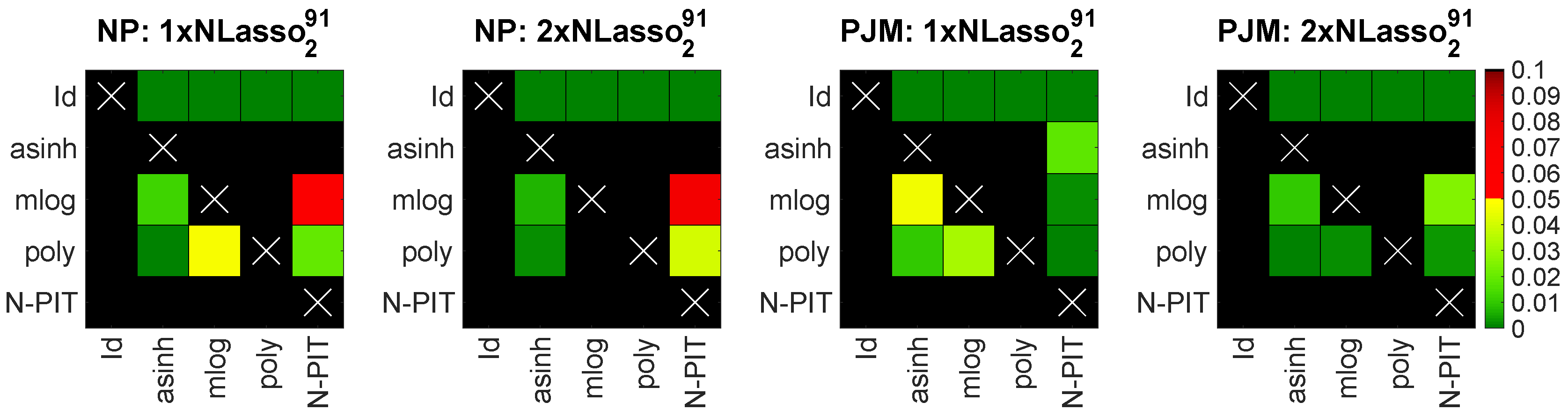
• The choice of the best performing transformation depends on the complexity of the model, e.g., for LASSO models based on bARX2, the asinh and N-PIT transformations led to the most accurate forecasts (see Table 1), and the benefit from using a VST increased with the complexity of the model. Moreover, for the two best performing models, a significant difference between using the asinh and N-PIT appeared only once (for PJM data) and it was in favor of the N-PIT transformation. Note, that both VSTs led to significantly better predictions than the remaining ones (see Figure 6).
• For almost all cases, models that re-estimate (reselect) $\lambda$ on a daily basis, i.e., $n\mathrm{xN}{\mathbf{LassOLS}}_i^D$ and $n\mathrm{xN}{\mathbf{Lasso}}_i^D$, outperformed models with a fixed tuning parameter, i.e., $n{\mathbf{LassOLS}}_i^D$ and $n{\mathbf{Lasso}}_i^D$, see Table 1 and Figure 4. On the other hand, re-estimating $\lambda$ is ca. 25 times slower (assuming that we have a grid of 25 $\lambda$s as we do here). The computational time can be reduced, however, by utilizing the results presented in Figure 7, i.e., by limiting the grid to 3–6 values of $\lambda$ for $D>60$ days.

To better understand the impact of applying a VST, it is necessary to refer to the article of Uniejewski et al. [16], where 16 transformations were tested across 12 datasets. Importantly, only models without exogenous variables were used in the cited study—an AR counterpart of our ARX2 and its neural network equivalent—and the price series were not decomposed into the LTSC and the stochastic component. The N-PIT turned out to be the best performing VST overall, at least in terms of MAE. However, for Nord Pool system prices covering a similar time period as in our study (30 July 2010 to 28 July 2016), the N-PIT was worse than asinh, mlog, and poly. Note that the same conclusion holds here for the autoregressive benchmarks (including ARX2). This suggests that the conclusions of Uniejewski et al. [16] are likely to remain unchanged when using a model with exogenous variables and/or a model that is fitted to deseasonalized series. From this perspective, the N-PIT gains the most from model complexity and even for more complex models, the N-PIT would probably outperform other VSTs.

4.3. Performance across $\lambda$-Selection Schemes

Up to this point, all LASSO-type models have used a 91-day validation window for selecting $\lambda$. A pertinent question arises as to whether this is the optimal choice for D. To address this, we considered eight validation window lengths: $D=1$ (one day), 7 (one week), 28 (one ‘month’), 60 (two months), 91 (one quarter), 182 (half a year), 273 (three quarters) and 364 (one year; this window is illustrated in Figure 1). On the other hand, the results discussed in Section 4.2 clearly show that (i) the bARX2 baseline model leads to significantly better performing LASSO-type models than the smaller bARX1 model, and (ii) $\ast {\mathbf{Lasso}}_i^{91}$ models significantly outperform $\ast {\mathbf{LassOLS}}_i^{91}$. Hence, to simplify the comparison, in this section, we limit the analysis to $\ast {\mathbf{Lasso}}_2^D$ models.

In

Table 2. Mean absolute errors (MAE) in the 631-day test period for 39 different $\lambda$-selection schemes (in rows), five VSTs (in columns; the first ‘transformation’ is identity, Id) and two markets (Nord Pool and PJM). A heat map is used to indicate better (→green) and worse (→red) results. Note that this time, the coloring is independent for each column to better emphasize the differences between the Ds.

, we report the MAEs in the 631-day test period for 39 different $\lambda$-selection schemes and five VSTs (including the identity ‘transformation’). Note that, as opposed to Table 1, now, the coloring is independent for each column to better emphasize the differences between the Ds. For both markets we can see the following:

• As observed in Section 4.2, models that re-estimate (reselect) $\lambda$ on a daily basis, i.e., $n\mathrm{xN}{\mathbf{Lasso}}_i^D$, outperform models with a fixed tuning parameter, i.e., $n{\mathbf{Lasso}}_i^D$. Yet, considering the significantly lower computational requirements, it is still reasonable to take the latter models as benchmarks.
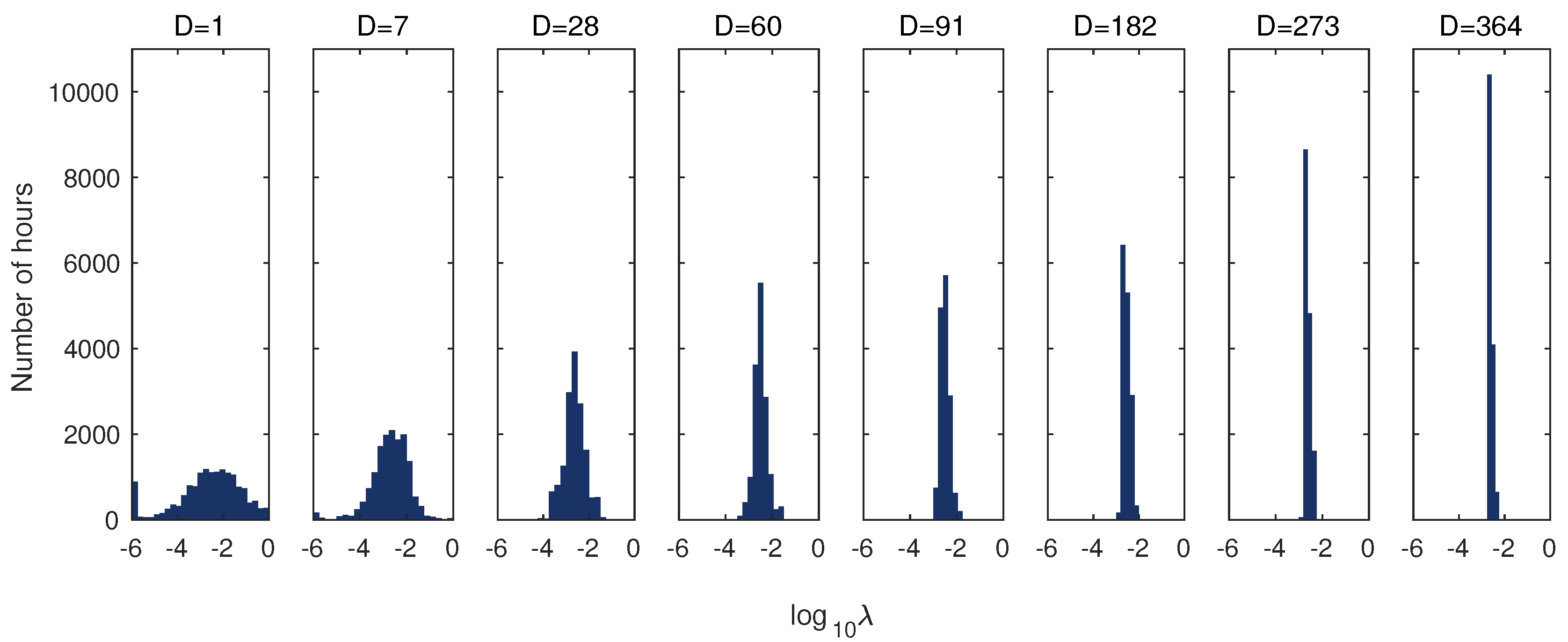
• As the length of the $\lambda$-selection window increases, the extreme values of the tuning parameter are less often selected and finally, for $D=364$ days, only a few intermediate $\lambda$s are used (for a sample illustration see Figure 7).
• Selecting validation windows of less than 60 days is not advisable. In the case of re-estimating (reselecting) $\lambda$s on a daily basis, i.e., in the $n\mathrm{xN}{\mathbf{Lasso}}_i^D$ models, it is recommended to use much longer validation windows.
• We cannot definitely reject or accept the hypothesis that choosing $\lambda$ for each hour separately leads to an improvement in the accuracy of the forecasts. Overall, the best results in terms of MAE were obtained for the 2xNLasso${}_2$ and 1xNLasso${}_2$ models and $D\ge 273$ days, but the differences between them and other well performing models were insignificant (DM test values are not reported here).

4.4. Variable Selection

Let us now comment on variable selection by looking at the 1xNLasso${}_2^{182}$ model calibrated to N-PIT-transformed data (the results for other $\ast {\mathbf{Lasso}}_2^D$, $D>60$ models were qualitatively similar). In

Table 3. Mean occurrence (in %) of model parameters across the 631-day test period. The columns represent the hours and the rows represent the parameters of the 1xNLasso${}_2^{182}$ model calibrated to N-PIT-transformed Nord Pool data. A heat map is used to indicate more (→ green) and less (→ red) commonly-selected variables.

(for Nord Pool) and

Table 4. Mean occurrence (in %) of model parameters across the 631-day test period. The columns represent the hours and the rows represent the parameters of the 1xNLasso${}_2^{182}$ model calibrated to N-PIT-transformed PJM data. A heat map is used to indicate more (→green) and less (→red) commonly-selected variables.

(for PJM), we present the mean occurrence (in %) of model parameters across the 631-day test periods. A heat map is used to indicate more (→green) and less (→red) commonly selected variables. Several interesting conclusions can be drawn.

• As reported in Uniejewski et al. [14] and Ziel and Weron [4], the price 24 h ago as well as the prices for the neighboring hours are important predictors (see the diagonals in rows 1–24 for day $d-1$ in Table 3 and Table 4). The diagonal was less visible around midday and for Nord Pool, it almost disappeared. The latter may be attributed to the explanatory power of the day-ahead wind prognosis for this market.
• Lagged prices for the more distant days ($d-2$ to $d-7$) were much less often selected, see Table 3 and Table 4. Although they cannot be ignored completely, particularly for days $d-2$ and $d-7$ for Nord Pool and day $d-7$ for PJM, it is hard to find any regular patterns that could be rationally (economically) justified.
• As observed by Maciejowska and Nowotarski [31] and Ziel [13], the price for hour 24 (i.e., $X_{d-1,24}$) is an important predictor. For on-peak hours, however, the evening prices (i.e., $X_{d-1,h}$ for $h=19,20,21,22$) seem to have more explanatory power. What is also surprising is that the morning prices (5 a.m. to 9 a.m.) on day $d-7$ provided more information than the evening prices on that day.
• The maximum prices on the previous seven days included more information than the minimum prices and for the Nord Pool dataset they were selected quite often (see the green cells in the bottom of Table 3). On the other hand, the minimum prices for day $d-1$ had high explanatory power for the early morning hours (1 a.m. to 7 a.m.; this effect was less pronounced for the PJM market).
• The exogenous variables (load and wind generation forecasts) for the past days were seldom selected. Only the forecasts for day d had high explanatory power and generally, only around the diagonal, i.e., for the same or neighboring hours.
• Finally, the dummies and the dummy-linked prices for the same hour and for midnight were important predictors (see Table 3 and Table 4). On the other hand, the dummy-linked load forecasts were of mixed importance, and the dummy-linked price averages for the previous day were usually removed by the LASSO (except for Tuesdays and Wednesdays for Nord Pool).

5. Conclusions

In this paper we presented a comprehensive empirical study on the optimal way of implementing the LASSO in electricity price forecasting that addresses the three open issues outlined in the Introduction. Concerning variable (or feature) selection, i.e., the optimal structure of the baseline model, we identified the most important variables and thus provided guidelines to structure better performing expert models. In particular, we found that large sets of potential regressors are not a problem for the LASSO procedure. Although the LASSO typically uses only a small fraction of the initial set of explanatory variables, providing additional information in the underlying model significantly improves the accuracy of the obtained forecasts. Nevertheless, lagged exogenous variables (i.e., load and wind generation forecasts for the past days) are seldom selected and can be ignored when building models. Only the day-ahead predictions for the target day have high explanatory power and generally, only for the same or neighboring hours. On the other hand, although lagged prices for the more distant days are much less often selected, they cannot be ignored completely (particularly days $d-2$ and $d-7$). We also confirmed the importance of dummies and the dummy-linked prices for the same hour and for midnight. At the same time, the dummy-linked load forecasts turned out to be of mixed explanatory power, while the dummy-linked price averages for the previous day were shown to be redundant.

Secondly, regarding the choice of the LASSO tuning parameter, we found one $\lambda$ for all days and hours in the test period (as in Uniejewski et al. [14]) to be an acceptable option, but this is recommended only if the computational time needs to be significantly reduced. To increase the forecast accuracy, it is better to reselect $\lambda$ on a daily basis. However, too frequent reselection (i.e., on an hourly basis, as in references [4,12,13]) is significantly outperformed by schemes that select only one or two (on-peak, off-peak) $\lambda$s per day, i.e., models 1xNLasso${}_2$ and 2xNLasso${}_2$, respectively. We also observed that despite a higher computational burden, it is extremely important to select $\lambda$ over periods of at least 60 days; however, cross-validation windows of half a year or more are recommended.

Thirdly, concerning the novel concept of variance stabilizing transformations (VSTs), we confirmed and reinforced the conclusions of Uniejewski et al. [16]. Namely, we showed that the VSTs not only increase the forecasting accuracy of LASSO-estimated models—like in the case of parsimonious regression and neural net models – but that the gains from using an appropriate VST increase with the complexity of the model. Lastly, using the Diebold–Mariano test, we found that for more complex models, it is advisable to use the asinh or the N-PIT transformation.

References

- Weron, R. Electricity price forecasting: A review of the state-of-the-art with a look into the future. Int. J. Forecast. 2014, 30, 1030–1081. [Google Scholar] [CrossRef]
- Karakatsani, N.; Bunn, D. Forecasting electricity prices: The impact of fundamentals and time-varying coefficients. Int. J. Forecast. 2008, 24, 764–785. [Google Scholar] [CrossRef]
- Misiorek, A. Short-term forecasting of electricity prices: Do we need a different model for each hour? Med. Econom. Toepass. 2008, 16, 8–13. [Google Scholar]
- Ziel, F.; Weron, R. Day-ahead electricity price forecasting with high-dimensional structures: Univariate vs. multivariate modeling frameworks. Energy Econ. 2018, 70, 396–420. [Google Scholar] [CrossRef] [Green Version]
- Amjady, N.; Keynia, F. Day-ahead price forecasting of electricity markets by mutual information technique and cascaded neuro-evolutionary algorithm. IEEE Trans. Power Syst. 2009, 24, 306–318. [Google Scholar] [CrossRef]
- Voronin, S.; Partanen, J. Price forecasting in the day-ahead energy market by an iterative method with separate normal price and price spike frameworks. Energies 2013, 6, 5897–5920. [Google Scholar] [CrossRef]
- Keles, D.; Scelle, J.; Paraschiv, F.; Fichtner, W. Extended forecast methods for day-ahead electricity spot prices applying artificial neural networks. Appl. Energy 2016, 162, 218–230. [Google Scholar] [CrossRef]
- Gianfreda, A.; Grossi, L. Forecasting Italian electricity zonal prices with exogenous variables. Energy Econ. 2012, 34, 2228–2239. [Google Scholar] [CrossRef] [Green Version]
- Barnes, A.K.; Balda, J.C. Sizing and economic assessment of energy storage with real-time pricing and ancillary services. In Proceedings of the 2013 4th IEEE International Symposium on Power Electronics for Distributed Generation Systems (PEDG), Rogers, AR, USA, 8–11 July 2013. [Google Scholar] [CrossRef]
- Ludwig, N.; Feuerriegel, S.; Neumann, D. Putting Big Data analytics to work: Feature selection for forecasting electricity prices using the LASSO and random forests. J. Decis. Syst. 2015, 24, 19–36. [Google Scholar] [CrossRef]
- González, C.; Mira-McWilliams, J.; Juárez, I. Important variable assessment and electricity price forecasting based on regression tree models: Classification and regression trees, bagging and random forests. IET Gener. Transm. Distrib. 2015, 9, 1120–1128. [Google Scholar] [CrossRef]
- Ziel, F.; Steinert, R.; Husmann, S. Efficient modeling and forecasting of electricity spot prices. Energy Econ. 2015, 47, 89–111. [Google Scholar] [CrossRef]
- Ziel, F. Forecasting Electricity Spot Prices Using LASSO: On Capturing the Autoregressive Intraday Structure. IEEE Trans. Power Syst. 2016, 31, 4977–4987. [Google Scholar] [CrossRef]
- Uniejewski, B.; Nowotarski, J.; Weron, R. Automated Variable Selection and Shrinkage for Day-Ahead Electricity Price Forecasting. Energies 2016, 9, 621. [Google Scholar] [CrossRef]
- Nowotarski, J.; Weron, R. On the importance of the long-term seasonal component in day-ahead electricity price forecasting. Energy Econ. 2016, 57, 228–235. [Google Scholar] [CrossRef]
- Uniejewski, B.; Weron, R.; Ziel, F. Variance Stabilizing Transformations for Electricity Spot Price Forecasting. IEEE Trans. Power Syst. 2018, 33, 2219–2229. [Google Scholar] [CrossRef]
- Diebold, F.X.; Mariano, R.S. Comparing predictive accuracy. J. Bus. Econ. Stat. 1995, 13, 253–263. [Google Scholar]
- Misiorek, A.; Trück, S.; Weron, R. Point and interval forecasting of spot electricity prices: Linear vs. non-linear time series models. Stud. Nonlinear Dyn. Econom. 2006, 10, 1558–3708. [Google Scholar] [CrossRef] [Green Version]
- Weron, R. Modeling and Forecasting Electricity Loads and Prices: A Statistical Approach; John Wiley & Sons: Chichester, UK, 2006. [Google Scholar]
- Marcjasz, G.; Uniejewski, B.; Weron, R. On the importance of the long-term seasonal component in day-ahead electricity price forecasting with NARX neural networks. Int. J. Forecast. 2018. [Google Scholar] [CrossRef]
- Uniejewski, B.; Marcjasz, G.; Weron, R. On the importance of the long-term seasonal component in day-ahead electricity price forecasting. Part II—Probabilistic forecasting. Energy Econ. 2018. [Google Scholar] [CrossRef]
- Janczura, J.; Trück, S.; Weron, R.; Wolff, R. Identifying spikes and seasonal components in electricity spot price data: A guide to robust modeling. Energy Econ. 2013, 38, 96–110. [Google Scholar] [CrossRef] [Green Version]
- Schneider, S. Power spot price models with negative prices. J. Energy Mark. 2011, 4, 77–102. [Google Scholar] [CrossRef] [Green Version]
- Diaz, G.; Planas, E. A Note on the Normalization of Spanish Electricity Spot Prices. IEEE Trans. Power Syst. 2016, 31, 2499–2500. [Google Scholar] [CrossRef]
- Hagfors, L.; Kamperud, H.; Paraschiv, F.; Prokopczuk, M.; Sator, A.; Westgaard, S. Prediction of extreme price occurrences in the German day-ahead electricity market. Quant. Financ. 2016, 16, 1929–1948. [Google Scholar] [CrossRef] [Green Version]
- Contreras, J.; Espínola, R.; Nogales, F.; Conejo, A. ARIMA models to predict next-day electricity prices. IEEE Trans. Power Syst. 2003, 18, 1014–1020. [Google Scholar] [CrossRef] [Green Version]
- Gaillard, P.; Goude, Y.; Nedellec, R. Additive models and robust aggregation for GEFCom2014 probabilistic electric load and electricity price forecasting. Int. J. Forecast. 2016, 32, 1038–1050. [Google Scholar] [CrossRef]
- Kristiansen, T. Forecasting Nord Pool day-ahead prices with an autoregressive model. Energy Policy 2012, 49, 328–332. [Google Scholar] [CrossRef]
- Maciejowska, K.; Nowotarski, J.; Weron, R. Probabilistic forecasting of electricity spot prices using Factor Quantile Regression Averaging. Int. J. Forecast. 2016, 32, 957–965. [Google Scholar] [CrossRef]
- Nowotarski, J.; Raviv, E.; Trück, S.; Weron, R. An empirical comparison of alternate schemes for combining electricity spot price forecasts. Energy Econ. 2014, 46, 395–412. [Google Scholar] [CrossRef]
- Maciejowska, K.; Nowotarski, J. A hybrid model for GEFCom2014 probabilistic electricity price forecasting. Int. J. Forecast. 2016, 32, 1051–1056. [Google Scholar] [CrossRef]
- James, G.; Witten, D.; Hastie, T.; Tibshirani, R. An Introduction to Statistical Learning with Applications in R; Springer: New York, NY, USA, 2013. [Google Scholar]
- Tibshirani, R. Regression shrinkage and selection via the lasso. J. R. Stat. Soc. B 1996, 58, 267–288. [Google Scholar]
Figure 1.
Nord Pool hourly system prices (top), hourly consumption prognosis (middle) and hourly wind power prognosis for Denmark (bottom) for the period 1 January 2013 to 19 September 2017. The vertical dashed lines mark the beginning of the 364-day period for selecting s for LASSO and the beginning of the 631-day long out-of-sample test period.
Figure 2.
Hourly prices for the Commonwealth Edison (COMED) zone in the PJM market (top), hourly system load forecasts (middle) and hourly zonal load forecasts for the COMED zone (bottom) for the period 1 January 2013 to 19 September 2017. The dashed lines have the same meaning as in Figure 1.
Figure 3.
Time series plots of the original (in EUR/MWh), asinh-transformed, mlog-transformed, poly-transformed and N-PIT-transformed Nord Pool spot prices (from top to bottom). All series were deseasonalized with respect to the S wavelet-based long-term seasonal component (LTSC) beforehand. The resulting marginal densities are depicted in the right panels.
Figure 4.
Results of the ‘multivariate’ variance stabilizing transformations (VSTs) multi-parameter Diebold–Mariano (DM) test for Nord Pool for the same 30 models as in Table 1 and the N-PIT transformation. A heat map is used to indicate the range of the p-values—the closer they are to zero (→dark green), the more significant the difference is between the forecasts of a model on the X-axis (better) and the forecasts of a model on the Y-axis (worse).
Figure 5.
Results of the ‘multivariate’ DM test for PJM for the same 30 models as in Table 1 and the N-PIT transformation. A heat map is used to indicate the range of the p-values—the closer they are to zero (→ dark green), the more significant the difference is between the forecasts of a model on the X-axis (better) and the forecasts of a model on the Y-axis (worse).
Figure 6.
Results of the ‘multivariate’ DM test for the best performers in Table 1 (i.e., and ) for Nord Pool (two left panels) and PJM (two right panels) across the VSTs. Like in Figure 4 and Figure 5, a heat map is used to indicate the range of obtained p-values for the pairwise comparisons.
Figure 7.
Histograms displaying the number of hours for which a given value of was selected in the whole Nord Pool test period ( h) across different Ds and for the N-PIT-transformed model. Recall, that we considered 25 exponentially decreasing s ranging from to ; they are plotted on a logarithmic scale on the X-axis. The histograms for PJM data look very similar (not plotted).