Load Forecasting for a Campus University Using Ensemble Methods Based on Regression Trees


1
Department of Applied Mathematics and Statistics, Universidad Politécnica de Cartagena, 30202 Cartagena, Spain
2
Department of Electrical Engineering, Universidad Politécnica de Cartagena, 30202 Cartagena, Spain
*
Author to whom correspondence should be addressed.
Energies 2018, 11(8), 2038; https://doi.org/10.3390/en11082038
Submission received: 6 July 2018
/
Revised: 1 August 2018
/
Accepted: 1 August 2018
/
Published: 6 August 2018
(This article belongs to the Special Issue Short-Term Load Forecasting by Artificial Intelligent Technologies)
Abstract
:Load forecasting models are of great importance in Electricity Markets and a wide range of techniques have been developed according to the objective being pursued. The increase of smart meters in different sectors (residential, commercial, universities, etc.) allows accessing the electricity consumption nearly in real time and provides those customers with large datasets that contain valuable information. In this context, supervised machine learning methods play an essential role. The purpose of the present study is to evaluate the effectiveness of using ensemble methods based on regression trees in short-term load forecasting. To illustrate this task, four methods (bagging, random forest, conditional forest, and boosting) are applied to historical load data of a campus university in Cartagena (Spain). In addition to temperature, calendar variables as well as different types of special days are considered as predictors to improve the predictions. Finally, a real application to the Spanish Electricity Market is developed: 48-h-ahead predictions are used to evaluate the economical savings that the consumer (the campus university) can obtain through the participation as a direct market consumer instead of purchasing the electricity from a retailer.
1. Introduction
Load forecasting has been a topic of interest for many decades and the literature is plenty with a wide variety of techniques. Forecasting methods can be divided into three different categories: time-series approaches, regression based, and artificial intelligence methods (see [1]).
Among the classical time-series approaches, the ARIMA model is one of the most utilized (see [2,3,4,5]). Regression approaches, see [2,6], are also widely used in the field of short-term and medium-term load forecasting, including non-linear regression [7] and nonparametric regression [8] methods. Recently, in [9] the authors use linear multiple regression to predict the daily electricity consumption of administrative and academic buildings located at a campus of London South Bank University.
Several machine learning or computational intelligence techniques have been applied in the field of Short Term Load Forecasting. For example, decision trees [10], Fuzzy Logic systems [11,12], and Neural Networks [13,14,15,16,17,18,19,20]. In this paper, we propose the using of a particular set of supervised machine learning techniques (called ensemble methods based on decision trees) to predict the hourly electricity consumption of university buildings. In general, an ensemble method combines a set of weak learners to obtain a strong learner that provides better performance than a single one. Four particular cases of ensemble methods are bagging, random forest, conditional forest, and boosting, which are described in Section 2. There some recent literature regarding random forest and short-term load forecasting: for example, in [21] the authors use random forest to predict the hourly electrical load data of the Polish power system, whereas in [22] the same method is used to predict residential energy consumption. In [23], the authors propose three different methods for ensemble probabilistic forecasting. The ensemble methods are derived from seven individual machine learning models, which include random forest, among others, and it is tested in the field of solar power forecasts. On the other hand, in [24] the authors establish a novel ensemble model that is based on variational mode decomposition and the extreme learning machine. The proposed ensemble model is illustrated while using data from the Australian electricity market.
The main objective of this paper is to illustrate the performance of different ensemble methods for predicting the electricity consumption of some university buildings, analyzing their accuracies, relevant predictors, computational times, and parameter selection. Besides, we apply the prediction results to the context of Direct Market Consumers (DMC) in the Spanish Electricity Market.
In Spain, electricity price seems to be above our European neighbors, mainly due to the energy production mix and the weak electrical interconnections with the Central European Electricity System and Markets, but consumers can do little about that. Therefore, it is quite challenging for Spanish consumers to reduce this cost. Currently, a high voltage consumer (voltage supply greater than 1 kV), which is the case of a small campus university, can opt for two types of supply: captive customer (price freely agreed with a retailer or a provider) and Direct Market Consumer (also called qualified customer), taking advantage of the operation of the wholesale markets that are involved in the Spanish Electricity System. The literature concerning the topic of DMC is nearly non-existent and it reduces to some official web pages, such as [25,26].
In order to participate as a DMC in the Electricity Market, the customer needs to evaluate his load requirements, with roughly two days in advance. Another objective of this paper is to evaluate the savings that the university would have participating as a DMC, taking the 48-h-ahead predictions of one of the ensemble methods analyzed.
The main differences among the present paper and the previous ones dealing with the using of ensemble methods for forecasting porpoises (for example, ref. [27] employs the gradient boosting method for modeling the energy consumption of commercial buildings) are the following: in the present paper, we propose the XGBoost method as a useful tool for a medium-size consumer to purchase the electricity directly in the wholesale market. For that, a different prediction horizon (48 h ahead) is considered and the new predictors are needed. Indeed, we highlight the importance of calendar variables (distinguishing different types of festivities) for the case of electricity consumption in university buildings. This approach allows us to evaluate the savings of this kind of customers participating as Direct Market Consumers. Another novelty respect to previous papers is the using of conditional forest as an ensemble method to get load predictions, as well as the conditional importance measure to evaluate the relevance of each feature.
Firstly, in Section 2, four ensemble methods based on regression trees are described. Section 3 depicts the customer in study (a small campus university) and the data, discusses the parameter selection for each ensemble method as well as other relevant aspects and it shows the prediction results. Finally, in Section 4, the economic saving of a small campus university is computed when it participates as a Direct Market Consumer instead of acquiring the electric power from a traditional retailer. Note that it is not an energy efficiency study, the economic saving is given just by the type of supply: retail or wholesale market.
2. Ensemble Methods Based on Regression Trees
Taking into account the type of data in the analysis (continuous data corresponding to electricity consumption), in this section, we will focus on describing tree-based methods for regression and some related ensemble techniques. However, decision trees and ensemble methods can be applied to both regression and classification problems.
The process of building a regression tree can be summarized in two steps: firstly, we divide the predictor space into a number of non-overlapping regions (for example J regions), and secondly, the prediction for a new observation is given by the mean of the response values of the training data belonging to the same region as the new observation.
The criterion to construct the regions or “boxes” is to minimize the residual sum of squares (RSS), but not considering every possible partition of the feature space into J boxes because it would be computationally infeasible. Instead, a recursive binary splitting is used: at each step, the algorithm chooses the predictor and cutpoint, such that the resulting tree has the lowest RSS. The process is repeated until a stopping criterion is reached, see [28].
Let be the training dataset, where each denotes the i-th output (response variable) and , the corresponding input of the “s” predictors (features) in study. The objective in a regression tree is to find boxes that minimize the RSS, given by (1):
where is the mean response for the training observations within the jth box.
A regression tree can be considered as a base learner in the field of machine learning. The main advantage of regression trees against lineal regression models is that in the case of highly non-linear and complex relationship between the features and the response, decision trees may outperform classical approaches. Although regression trees can be very non-robust and can generally provide less predictive accuracy than some of the other regression methods, these drawbacks can be easily improved by aggregating many decision trees, using methods, such as bagging, random forests, conditional forest, and boosting. These four methods have in common that can be considered as ensemble learning methods.
An ensemble method is a Machine Learning concept in which the idea is to build a prediction model by combining a collection of “N” simpler base learners. These methods are designed to reduce bias and variance with respect to a single base learner. Some examples of ensemble methods are bagging, random forest, conditional forest, and boosting.
2.1. Bagging
In the case of bagging (bootstrap aggregating), the collection of “N” base learners to ensemble is produced by bootstrap sampling on the training data. From the original training data set, N new training datasets are obtained by random sampling with replacement, where each observation has the same probability to appear in the new dataset. The prediction of a new observation with bagging is computed by averaging the response of the N learners for the new input (or majority vote in case of classification problems). In particular, when we apply bagging to regression trees, each individual tree has high variance, but low bias. Averaging the resulting prediction of these N trees reduces the variance and substantially improves in accuracy (see [28]).
The efficiency of the bagging method depends on a suitable selection of the number of trees N, which can be obtained by plotting the out-of-bag (OOB) error estimation with respect to N. Note that the bootstrap sampling step with replacement involves that each observation of the original training dataset is included in roughly two-thirds of the N bagged trees and it is out of the remaining ones. Then, the prediction of each observation of the original training dataset can be obtained by averaging the predictions of the trees that were not fit using that observation. This is a simple way, called OOB, to get a valid estimate of the test error for the bagged model avoiding a validation dataset or cross-validation.
Some other parameters that can also vary are the node size (minimum number of observations of the terminal nodes, generally five by default) and the maximum number of terminal nodes in the forest (generally trees are grown to the maximum possible, subject to limits by node size).
In this paper, the bagging method has been applied by means of the R package “randomForest”, see [28]. The package also includes two measures of predictor importance that help to quantify the importance of each predictor in the final forecasting model and might suggest a reduced set of predictors.
2.2. Random Forest
Random forests are indeed a generalization of bagging. Instead of considering all of the predictors at each split of the tree, only a random sample of “mtry” predictors can be chosen each time. The main advantage of random forests respect to bagging can be noticed in the case of correlated predictors, as it is stated in [28]: predictions from the bagged trees will be highly correlated so that bagging will not reduce the variance so much, whereas random forests overcome this problem by forcing each split to consider only a subset of the predictors.
In the case of random forest, the efficiency of the method depends on a suitable selection of the number of trees N and the number of predictors mtry tested at each split. Again, the OOB error can be used for searching a suitable N as well as a suitable mtry. As with bagging, random forests will not overfit if we increase N, so the goal is to choose a value that is sufficiently large. The random forest method that is used in this paper has been implemented throughout the R package “randomForest”, see [29].
2.3. Conditional Forest
Conditional forests consist in an implementation of the bagging and random forest ensemble algorithms, but utilizing conditional inference trees as base learners. Conditional inference trees are not only suitable for prediction (its partitioning algorithm avoid overfitting), but also for explanation purposes because they select variables in an unbiased way. They are especially useful in the presence of high-order interactions and when the number of predictors is large when compared to the sample size.
In conditional forests, each tree is obtained by binary recursive partitioning, as follows (see [30]): firstly, the algorithm tests whether any predictor is associated with the response, and it chooses the one that has the strongest association; secondly, the algorithm makes a binary split in this variable; finally, the previous two steps are repeated for each subset until there are no predictors that are associated with the response. The first step uses the permutation tests for conditional inference developed in [31].
As with random forest, in the case of conditional forest, we need a suitable selection of the number mtry of features tested at each split (the total number of predictors might be preferred) and the number of trees N (generally a lower value than for random forest is required). In this paper, the conditional forest method has been implemented throughout the R package “party”, see [32].
2.4. Boosting
In contrast to the above ensemble methods, in boosting the “N” base, learners are obtained sequentially, that is, each base learner is determined while taking into account the success and errors of the previous base learners.
The first boosting algorithm was Adaptive Boosting (AdaBoost), as introduced in [33]. Instead of using bootstrap sampling, the original training sample is weighted at each step, giving more importance to those observations that provided large errors at previous steps. Besides, the prediction for a new observation is given by a weighted average (instead of a simple average) of the responses of the N base learners.
AdaBoost was later recast in a statistical framework as a numerical optimization problem where the objective is to minimize a loss function using a gradient descent procedure, see [34]. This new approach was called “gradient boosting”, and it is considered one of the most powerful techniques for building predictive models.
Gradient boosting involves three elements: a loss function to be optimized, a weak learner to make predictions (in this case, decision trees obtained in a greedy manner), and an additive model to add weak learners (the output for each new tree is added to the output of the existing sequence of trees). The loss function used depends on the type of problem. For example, a regression problem may use a squared error loss function, whereas a classification problem may use logarithmic loss. Indeed, any differentiable loss function can be used.
Although boosting methods reduces bias more than bagging, they are more likely to overfit a training dataset. To overcome this task, several regularization techniques can be applied.
- Tree constraints: there are several ways to introduce constraints when constructing regression trees. For example, the following tree constraints can be considered as regularization parameters:
- ○
- The number of gradient boosting iterations N: increasing N reduces the error on the training dataset, but may lead to overfitting. An optimal value of N is often selected by monitoring prediction error on a separate validation data set.
- ○
- Tree depth: the size of the trees or number of terminal nodes in trees, which controls the maximum allowed level of interaction between variables in the model. The weak learners need to have skills but they should remain weak, thus shorter trees are preferred. In general, values of tree depth between 4 and 8 work well and values greater than 10 are unlikely to be required, see [35].
- ○
- The minimum number of observation per split: the minimum number of observations needed before a split can be considered. It helps to reduce prediction variance at leaves.
- Shrinkage or learning rate: in regularization by shrinkage, each update is scaled by the value of the learning rate parameter “eta” in (0,1]. Shrinkage reduces the influence of each individual tree and leaves space for future trees to improve the model. As it is stated in [28], small learning rates provide improvements in model’s generalization ability over gradient boosting without shrinking (eta = 1), but the computational time increases. Besides, the number of iterations and learning rate are tightly related: for a smaller learning rate “eta”, a greater N is required.
- Random sampling: to reduce the correlation between the trees in the sequence, at each step, a subsample of the training data is selected without replacement to fit the base learner. This modification prevent overfitting and it was first introduced in [36], which is also called stochastic gradient boosting. Friedman observed an improvement in gradient boosting’s accuracy with samplings of around one half of the training datasets. An alternative to row sampling is column sampling, which indeed prevents over-fitting more efficiently, see [37].
- Penalize tree complexity: complexity of a tree can be defined as a combination of the number of leaves and the L2 norm of the leaf scores. This regularization not only avoids overfitting, it also tends to select simple and predictive models. Following this approach, ref. [37] describes a scalable tree boosting system called XGBoost. In that paper, the objective to be minimized is a combination of the loss function and the complexity of the tree. In contrast to the previous ensemble methods, XGBoost requires a minimal amount of computational resources to solve real-world problems.
In XGBoost, the model is trained in an additive manner and it considers a regularized objective that includes a loss function and penalizes the complexity of the model. Following [37], if we denote by , the prediction of the i-th instance of the response at the t-th iteration, we need to find the tree structure that minimizes the following objective:
In the first term of (2), l is a differentiable convex loss function that measures the difference between the observed response and the resulting prediction . The second term of (2) penalizes the complexity of the model, as follows:
where T is the number of leaves in the tree with leaf weights Using the second order Taylor expansion, (3) can be simplified to:
where and .
Denoting by the instance set of leaf j, we can rewrite (4), as follows:
Therefore, the optimal weight is given by:
and the corresponding optimal objective by:
where q represents the optimal tree structure with T leaves and leaf weights
Due to the impossibility of enumerating all the possible tree structures q, a greedy algorithm is used (it starts with a single leaf and adds branches iteratively). Denoting by IL and IR the instance sets of left and right nodes after the split, , the reduction in the objective after the split is given by:
The task of searching the best split has been developed in two scenarios: an exact greedy algorithm (it enumerates all the possible splits on all the features, which is computational demanding) and an approximate greedy algorithm for big data sets, see [37] for more details.
The main difference between random forest and boosting is that the former builds the base learners independently through bootstrap sampling on the training dataset, while the latter obtains them sequentially focusing on the errors of the previous iteration and using gradient descent methods. Some strengths of the XGBoost implementation comparing to other methods are:
- An exact greedy algorithm is available.
- Approximate global and approximate local algorithms are available for big datasets.
- It performs parallel learning. Besides, an effective cache-aware block structure is available for out-of-core tree learning.
- It is efficient in case of sparse input data (including the presence of missing values).
The extreme gradient boosting method (XGBoost) has been implemented by means of the R package “xgboost”, see [38].
Apart from its highly computational efficiency, the XGBoost offers a great flexibility, but it requires setting up more than the ten parameters that could not be learned from the data. Taking into account that R package “xgboost” does not have any hyperparameter tuning, the parameter tuning can be done by means of cross validation. However, creating a grid for all of the parameters to be tuned implies an extremely high computational cost.
3. Prediction Results for the University Buildings
In this section, the four ensemble methods that are described above are applied to the electricity consumption of a small campus university to evaluate the adequacy of each technique in this type of customers. Specifically, we will focus on 48-h-ahead predictions in order to apply them to the context of Direct Market Consumers, although different prediction horizons will be also considered for the case of XGBoost method. Some other aspects, such us predictors importance or parameter selection, for each method are also developed.
Firstly, in this section, the customer in study is introduced. Secondly, the load data, predictors, and some goodness of fit measurements are depicted. Finally, the forecasting results for the case study are shown.
3.1. Customer Description: A Campus University
The campus “Alfonso XIII” of the Technical University of Cartagena (UPCT, Spain) comprises seven buildings ranging from 2000 m2 to 6500 m2 and a meeting zone (10,000 m2). Buildings are of two kinds: naturally ventilated cellular (individual windows, local light switches, and local heating control) and naturally ventilated open-plan (office equipment, light switched in longer groups, and zonal heating control). This campus has an overall surface larger than 35,500 m2 to fulfill the needs of different Faculties for classrooms, departmental offices, administrative offices, and laboratories for 1800 students and 200 professors. Unfortunately, the age of buildings (50 years old in four cases) and architectural conditioning works are far from actual energy efficiency standards, specifically in the two main electrical end-uses of the building: air conditioning/space heating (low performance, insufficient heat insulation, and an important cluster of individual appliances for offices and small laboratories) and lighting (where conventional magnetic ballasts and fluorescent are still used at a great extend).
With respect to the share of end-uses in the “Campus Alfonso XIII” of UPCT, heating, ventilation, and air conditioning (HVAC) is the largest energy end-use (this trend is the same both in the residential and non-residential buildings in Spain and other countries, see Table 1) with 40–50% of overall demand; lighting follows with 25–30%, electronics and office equipment 7–12% and other appliances with 8–10% (i.e., vending machines, refrigeration, water heaters WH, laboratory equipment, etc.). Notice that building type is critical in how energy end uses are distributed in each specific building. Table 1 shows a comparative of end-uses in office buildings in three countries [39] and in the analysed case, campus “Alfonso XIII”.
3.2. Data Description
Data used in this paper correspond to the campus Alfonso XIII of the Technical University of Cartagena, as described in the previous subsection. Hourly load data from 2011 to 2016 (both included) were analyzed, obtained from the retailer electric companies (Nexus Energía S.A. and Iberdrola S.A.). It is well known that electricity consumption is related to several exogenous factors, such as the hour of the day, the day of the week, or the month of the year, and therefore these factors must be taken into account in the design of the prediction model. Temperature is a factor that might affect the electricity consumption (cooling and heating of the university buildings). Thus, the hourly temperature was considered as an input in the forecasting model, as provided by AEMET (Agencia Española de Meteorología) for the city of Cartagena (where the campus university is located), from 2011 to 2016. Besides, depending on the end-uses of the customer in study, some other features can be relevant for the load. For example, in this case study, different types of holidays or special days have been distinguished throughout binary variables (see Table 2 for a detailed description).
Three different measurements given in (9), (10), and (11) were used to obtain the accuracy of the forecasting models: the root mean square error (RMSE), the R-squared (percentage of the variability explained by the forecasting model), and the mean absolute percentage error (MAPE). Although the MAPE is the most used error measure, see [1], the squared error measures might be more fitting because the loss function in Short Term Load Forecasting is not linear, see [13]. Some descriptive measures of the errors (such as the mean, skewness, and kurtosis) were also considered to evaluate the performance of the forecasting methods.
The root mean square error is defined by:
the R-squared is given by:
and the mean absolute percentage error is defined by:
where is the number of data, is the actual load at time , and is the forecasting load at time .
3.3. Forecasting Results
Data from 1 January 2011 to 31 December 2015 were selected as the training period in all methods, whereas data from 1 January 2016 to 31 December 2016 constituted the test period. In this subsection, firstly a prediction horizon of 48 h is established, whose forecasting results will be used in the next section dealing with Direct Market Consumers. In this case, we consider 53 predictors (see Table 2): 23 dummies for the hour of the day, six dummies for the day of the week, 11 dummies for the month of the year, five dummies for special days (FH1, …, FH5), two predictors of historic temperatures (lags 48 h and 72 h), and six predictors of historic loads (lags 48 h, 72 h, 96 h, 120 h, 144 h, and 168 h).
For each ensemble method, the parameter selection has been developed and measures of variable importance have been obtained (see Table 3 for the meaning of each term). In order to have reproducible models and comparable results, the same seed was selected in all procedures that require random sampling. In the case of bagging and random forest, we have selected an optimal number of trees (ntree) through the OOB error estimate and we have ordered the predictors according to the node impurity importance measure, see [28]. For bagging, the number of predictors that are considered at each split must be the total number of predictors, whereas in the case of random forest, the optimal parameter has been selected using the OOB error estimate for different values of mtry. In the case of conditional forest, the conditional variable importance measure introduced in [40] has been considered, which better reflects the true impact of each predictor in presence of correlated predictors.
While in bagging and random forest the OOB error was used to tune the parameters, in the case of conditional forest and XGBoost the parameters were tuned by means of cross validation with five folds (approximately one year in each fold). As for conditional forest, only two parameters need to be tuned (ntree and mtry), but in XGBoost, there are more parameters to tune. Although one can apply cross validation taking into account a multi-dimension grid with all of the parameters to tune (this approach would imply a high computational cost), we considered a simplification of the search selecting subsample = 0.5, max depth = 6 (appropriate in most problems) and looking for a good combination of “eta” and “nrounds”, see Table 4. The rest of parameters of the method were set up by default, according to the R package [38]. In the case of XGBoost, features have been ordered by decreasing importance while using the gain measure defined in [36].
Table 4 shows the results of the parameter selection for the XGBoost method. Recall that a lower learning rate eta implies a greater number of iterations nround, but a too large nround can lead to overfitting. Combination (eta = 0.02, nrounds = 3400) provided the lowest RMSE and the highest R-squared scores for the test data, whereas (eta = 0.01, nrounds = 5700) got the lowest MAPE. However, any pair of parameters in Table 4 could be appropriate because they lead similar accuracy.
Table 5 and Table 6 show the results that were obtained for the best parameter selection of each ensemble method. They also include the comparison with traditional and simple forecasting models, such as naïve (prediction at hour h is given by the real consumption at hour h-168) and multiple linear regression (MLR) with the same predictors, as used in the ensemble methods. According to Table 5, XGBoost method provides nearly null bias, more symmetry of the errors than the other ensemble methods and the traditional ones, as well as values of the kurtosis that are closer to zero (considered desired properties for residual in forecasting techniques).
Although bagging and random forest provide the best accuracy in the training dataset (see Table 6), XGBoost fits better in the test dataset (in this case, gradient boosting avoid more overfitting than the others ensemble methods due to a suitable selection of the parameters). Furthermore, when comparing the results of random forest and XGBoost, we can state that the latter fits lightly better and it is twelve times faster to compute. Table 6 also shows that all ensemble methods significantly improve the accuracy of the predictions with respect to MLR and naïve models.
It is also important to remark that, for all methods, roughly half of the predictors accumulate more that 99% of the relative importance. In the case of ensemble methods, the corresponding importance measure has been computed (for example, the node impurity for random forest and the gain for XGBoost), whereas in the case of MLR, the forward stepwise selection method and R-squared were used to evaluate the relative importance of each predictor. We can also highlight the following aspects: the electricity consumption at the same hour of the previous week (predictor LOAD_lag_168) results the most important feature in all methods, the electricity load with lags 48 h and 144 h appear among the five most important predictors in all of the ensemble methods, and finally, the presence of the features WH6, WH7, FH1, and FH3 among the five most important predictors for different methods evidences that calendar variables and types of holidays are essential for this kind of customer. However, the temperature has a reduced effect on the response because it appears between the 10th and 12th position of importance (depending on the method), with a relative importance of around 1%.
In order to compare the accuracy for the different types of day, the days of the test data (2016) were divided in two groups: special days, which include weekends, August (official academic holidays), and all days that are determined by the dummy variables FH1, …, FH5 in Table 2; and, regular days, which include the rest of the days. Results are exposed in Table 7. Notice that the lowest MAPE scores are always reached for regular days.
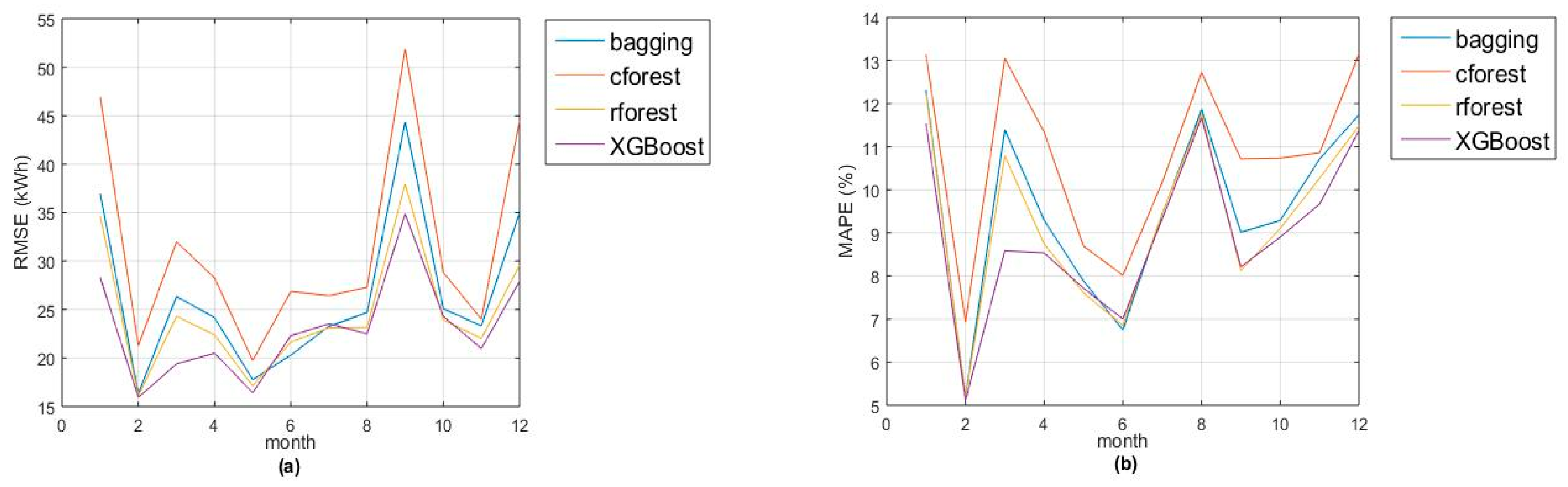
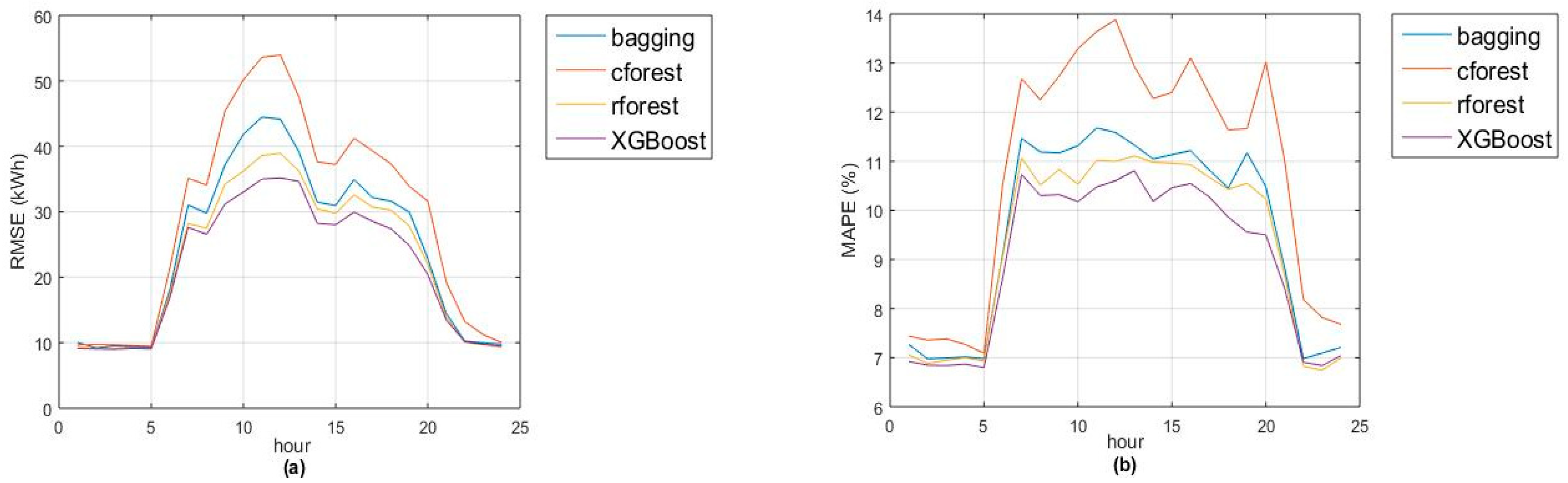
Figure 1a,b show the monthly evolution of two goodness-of-fit measures (RMSE and MAPE). Remark that accuracies of random forest and XGBoost are quite similar, with greatest differences in January and March (due to lack of accuracy in Christmas and Eastern days). Also, the models fit better for night hours (from 10 p.m. to 5 a.m.) due to the absence of activity during that period (see Figure 2a,b).
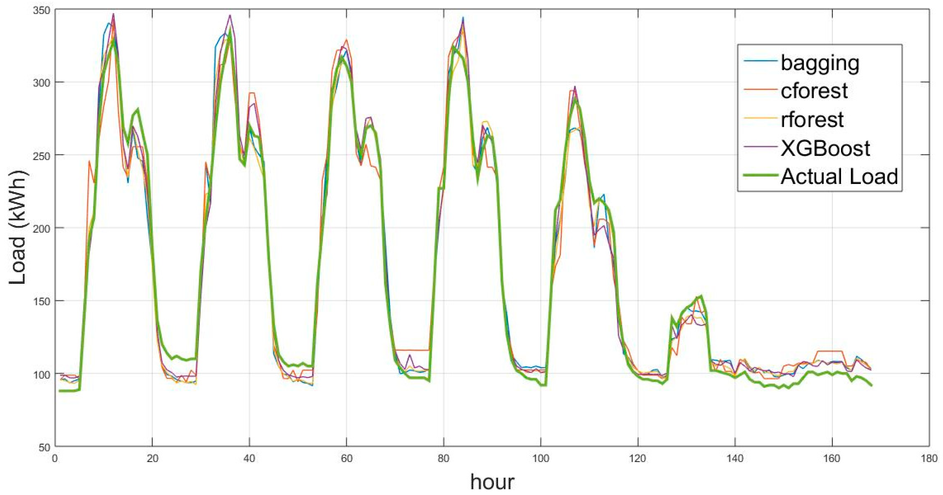
As an example, Figure 3 shows the actual and prediction load for a complete week in May 2016.
Finally, in this section, we analyze the adecuacy of the forecasting method XGBoost for the case study when considering different prediction horizons (1 h, 2 h, 12 h, 24 h, and 48 h). In all cases, we selected the same parameters: subsample = 0.5, max_depth = 6, eta = 0.05 and nrounds = 1700. Accuracy results for the training and test datasets are given in Table 8 as well as the most important predictors in each case.
Obviously, the best accuracies are obtained for the shortest prediction horizon (1 h), where the most important feature is the consumption at the previous hour (lag = 1) with more than 85% of relative importance. However, for the rest of prediction horizons, the most important predictor is, once again, the load with lag 168 h.
4. Direct Market Consumers
Direct Consumers in the market by point of supply or installation are those consumers of electric energy who purchase electricity directly on the production market for their own consumption and who meet some specific conditions. Firstly, this section is dealing with the performance of the Spanish Market, specifically the aspects that are related to DMC type of supply. Secondly, the components that define the price of the energy as a DMC are introduced. Finally, the results for the case of a campus university are shown.
4.1. Law Framework for DMC and Market Performance
Law 24/2013 of 26 December [41] defines the Direct Consumers in the Spanish Market in article 6.g) and establishes its rights and obligations. The activity of these subjects is regulated in Royal Decree 1955/2000 of 1 December [42], which regulates the activities of transportation, distribution, retailing, supply, and authorization procedures of Power Systems. To start the activity of qualified consumer in the market, the interested party must send several documents to different official bodies and fulfill a series of requirements, such as: have provided the System Operator with sufficient guarantee to cover economic obligations and to have the status of market agent, among others. Currently, the list of DMC includes around 200 consumers, most of them small and medium companies (see [43]).
The Day-ahead Market, as part of the electric power production market, aims to carry out electric power transactions for the next day by resolving offers and bids that are offered by market agents. The Market Operator ranks and matches selling offers with buying bids for electricity (received before 10:00 a.m. on the day before the dispatch), using the simple or complex matching method, according to simple or there are offers that incorporate complex conditions.
According to that, DMC must make their bids for the day D (day of dispatch) before 10:00 a.m. of day D-1 (day before the dispatch), so nearly two-day-ahead forecasting models for the demand are needed. After this process, the System Operator established the Daily Base Program, which is published at 12:00, based on the program resulting from the Market Operator program for the Day-Ahead Market and the communication of the execution of bilateral contracts. The Intraday Market aims to meet the Definitive Viable Daily Program through the presentation of energy offers and bids by the markets agents. The final scheduling is the result of the aggregation of all the firm transactions that are formalized for each programming period as a consequence of the viable daily program and market matching intraday once the technical restrictions identified have been resolved and the subsequent rebalancing has taken place. Finally, generation and demand deviations arising from the closing of the final scheduling are managed by the System Operator through balance management procedures and the provision of secondary and tertiary regulation services.
4.2. Price of the Energy Participating as a DMC
The final price of the energy consumed as a DMC consists of three clearly differentiated components, as described below.
- Regulated prices: these are prices set by the State and also depend on the supply rate. This component includes access fees, capacity payments and loss coefficients. This component does not depend on the type of supply, thus the corresponding cost would be the same for consumers through retailers and DMC.
- Taxes: they are also regulated prices, although of a different nature from the previous ones. This component is given by the special tax on electricity (currently 5113%) and VAT (currently 21%). This component is also common for all consumers.
- Unregulated prices: this component of the billing contemplates the price for the energy consumed in wholesale market and therefore it is not regulated by the State. It includes the price of energy in the Day-ahead and Intraday Market, costs for bilateral contracts, costs for measured deviations (difference between energy consumed and programmed energy), and costs for ancillary services.
Therefore, the Final Cost of the energy for a Direct Market Consumer is given by:
The price of energy in the Day-ahead or Daily Market, which is also called the marginal price, is the result of matching sales and purchase offers managed the day before the energy dispatch. It is therefore a non-regulated component of the billing. The price of energy in the Day-ahead Market is determined for each of the 24 h of the day as a result of the matching, values that are available on the website of the System Operator [44] (Red Eléctrica Española, REE). It is the largest component (more than 80%) of the average final price, as it is shown in Figure 4.
As in the Daily Market, the price of energy in the Intraday Market is the result of the negotiation of sales and purchase offers managed in the sessions held a few hours before the dispatch of energy (intraday sessions), and both are variable and unregulated prices. The price for each hour of the day and each intraday session are posted on the website of the System Operator, in this case REE [44].
Once the daily scope of the agents, consumers, and generators programs has been reached, the processes of liquidation of their energies (charges and payments) actually produced and consumed are entered, with each passing the costs of the deviation that they have incurred by have “failed” their respective programs of production and consumption. Thus, those who have deviated to rise at a certain time (generators that have produced more than their program and consumers who have consumed less than their programs) are passed on the corresponding cost in case that deviation has gone in the opposite direction (the generators charge a price lower than the marginal price of the hour for their additional production, and consumers receive a price lower than the marginal price they paid in that hour for their lower consumption), while if their deviation was in the same sense of the needs of the system, no cost is passed on to them (generators charge the marginal and consumers receive the marginal). Identical reasoning governs the case of deviations to go down, in which producers have generated less energy than their program and consumers have consumed more than what is established in their schedule.
In order to compare the real electricity bill in 2016 of the customer (the campus university) with the one that it would have had acting as a DMC, the parts that are different in both of the bills have been emphasized. The real electricity bill emitted by the supplier in 2016 (a retailer) consists of three components: the access fees (regulated price), the taxes, and the “referenced energy” (which includes some regulated prices such as the capacity payments or loss coefficients and all of the unregulated prices).
Taking into account that the access fees and taxes are the same for the two types of supply (retailer and DMC), the cost of the “referenced energy” for 2016 is analyzed.
For a DMC, the hourly cost of the (referenced) energy is given by the following sum of costs:
where:
- E(h) = Energy cost in the hour “h”, in €.
- ECBC(h) = Energy cost in the hour “h” from bilateral contracts, in €.
- DMP(h) = Daily Market price in the hour “h”, in €/kWh.
- EDM(h) = Energy bought in the Daily Market in the hour “h”, in kWh.
- IMP(h) = Intraday Market price in the hour “h”, in €/kWh.
- EIM(h) = Energy bought in the Intraday Market in the hour “h”, in kWh.
- SAC(h) = System adjustment cost passed on to the DMC in the hour “h”, in €/kWh.
- EMCB(h) = Energy measured in Central Bars in the hour “h”, in kWh.
- MDP(h) = Measured Deviations price in the hour “h”, in €/kWh.
- EMD(h) = Measured Deviation of Energy in the hour “h” = Difference between consumed energy and programmed energy in the hour “h”, in kWh.
- CPP(h) = Capacity payment price in the hour “h”, in €/kWh.
In this paper, it is assumed that the DMC in the study (the campus university) does not participate in bilateral contracts nor in the Intraday Market, thus the hourly cost of the energy reduces to:
It is mandatory for the Spanish Regulator (Comisión Nacional del Mercado y la Competencia, CNMC) to publish on its website a document with the criterion used to calculate the average final price (AFP) of energy in the market. The AFP (see Figure 4) represents an approximate value of the cost of electric energy per kWh, being only a reference that can vary to a greater or lesser extent from the actual final price, depending on the consumer. Specifically, the capacity payments and the deviations between energy consumed and programmed, are those that can mark greater differences between the real cost of the invoicing and the cost resulting from using the average final price. As an additional objective, we compare the real cost acting as a DMC with the resulting cost using the AFP.
4.3. Case Study: A Campus University as a DMC
To date, all the dependencies of the Technical University of Cartagena have contracted supply with a retailer, which is the modality of supplying of almost all consumers in high voltage of the Spanish electrical system. Only around 200 consumers have dared to participate in the Market as DMC, see the list in [43]. In 2016, the contracted tariff for the Alfonso XIII campus was the ATR 6.1, 6-period high voltage tariff, with a supply voltage of 20 kV.
As it has been stated before, the final price of the campus university’s invoice is composed of the access fees (which refers to the use of the network), the taxes, and the price of the energy freely agreed with the retailer (which refers to the value of the energy consumed). Note that the concepts corresponding to access fees (power and energy terms) and taxes are independent of the mode of supply, so they do not change for a Direct Consumer. Therefore, the calculation of the cost of the referenced energy for the DMC and its comparison with the retailer cost, is the main concern for this study.
Recall that, under the assumptions of this study, the hourly energy cost as a DMC is given by the sum of four components: the cost in the Daily Market (DM cost), the adjustment services (AS cost), the measured deviations (MD cost), and the capacity payments (CP cost). Table 9 shows the value of each component when the cost of the energy as a DMC is evaluated. In this section, 48-h-ahead predictions obtained with the XGBoost method (eta = 0.02, nrounds = 3700) were used, although any of the other ensemble methods would lead to similar results. It is worth to mention that the cost of deviations is quite limited due to the accuracy of the load forecasting method.
Table 10 shows the electricity consumption (in kWh) of the campus university in 2016 and the cost of the referenced energy (consumption) in four cases: the real cost paid to the retailer, the cost using the Average Final Price (AFP), acting as a DMC, and what we call the pessimist price (a Direct Consumer with all the deviations against the system). According to the results, it can be established that DMC modality would have produced savings of around 11% in the energy term of the invoice when compared to the retail price. Note also that the cost using the AFP does not coincide with the cost of the DMC because the cost due to deviations and the capacity payments components depend on the consumer. On the other hand, the results show that, even in the pessimistic case (all deviations of the predictions against the system), the DMC type of supply is worthy against the retailer.
It is important to highlight that the economic benefits of the DMC type of supply depend on two main aspects: the magnitude of the deviations and the direction of the deviations (towards or against the system). The first aspect (magnitude of the deviations) is determined by the accuracy of the forecasting method. However, the second aspect (direction of the deviations) is out of our control and it depends on the whole Electric System. In particular, some worse forecasting methods could lead to greater benefits than more accuracy methods, but only by chance and assuming that the forecasting values are good enough (moderate deviations). Therefore, the load forecasting method is important to some extent, but obviously lower deviations are preferable to greater deviations.
5. Conclusions
Load forecasting has been an important concern to provide accurate estimates for the operation and planning of Power Systems, but it can also arise as an important tool to engage and empower customers in markets, for example for decision making in electricity markets.
In this paper, we propose the using of different ensemble methods that are based on regression trees as alternative tools to obtain short-term load predictions. The main advantages of this approach are the flexibility of the model (suitable for linear and non-linear relationships), they take into account interactions among the predictors at different levels, no assumption or transformations on the data are needed, and they provide very accurate predictions.
Four ensemble methods (bagging, random forest, conditional forest, and boosting) were applied to the electricity consumption of the campus Alfonso XIII of the Technical University of Cartagena (Spain). In addition to historical load data, some calendar variables and historical temperatures were considered, as well as dummy variables representing different types of special days in the academic context (such as exams periods, tutorial periods, or academic festivities). The results show the effectiveness of the ensemble methods, mainly random forest, and a recent variant of gradient boosting called the XGBoost method. It is also worth to mention the fast computational time of the latter.
To illustrate the utility of this load-forecasting tool for a medium-size customer (a campus university), predictions with a horizon of 48h were obtained to evaluate the benefits that are involved in the change from tariffs to price of wholesale markets in Spain. This possibility provides an interesting option for the customer (a reduction of around 11% in electricity costs).
Author Contributions
M.d.C.R.-A. and A.G. (Antonio Gabaldón) conceived, designed the experiments and wrote the part concerning load forecasting. A.G. (Antonio Guillamón) and M.d.C.R.-A. collected the data, developed and wrote the part concerning the direct market consumer. All authors have approved the final manuscript.
Funding
This research was funded by the Ministerio de Economía, Industria y Competitividad (Agencia Estatal de Investigación, Spanish Government) under research project ENE-2016-78509-C3-2-P, and EU FEDER funds. The third author is also partially funded by the Spanish Government through Research Project MTM2017-84079-P (Agencia Estatal de Investigación and Fondo Europeo de Desarrollo Regional). Authors have also received funds from these grants for covering the costs to publish in open access.
Acknowledgments
This work was supported by the Ministerio de Economía, Industria y Competitividad (Agencia Estatal de Investigación, Spanish Government) under research project ENE-2016-78509-C3-2-P, and EU FEDER funds. The third author is also partially funded by the Spanish Government through Research Project MTM2017-84079-P (Agencia Estatal de Investigación and Fondo Europeo de Desarrollo Regional). Authors have also received funds from these grants for covering the costs to publish in open access.
Conflicts of Interest
The authors declare no conflict of interest.
References
- Hahn, H.; Meyer-Nieberg, S.; Pickl, S. Electric load forecasting methods: Tools for decision making. Eur. J. Oper. Res. 2009, 199, 902–907. [Google Scholar] [CrossRef]
- Alfares, H.K.; Nazeeruddin, M. Electric load forecasting: Literature survey and classification of methods. Int. J. Syst. Sci. 2002, 33, 23–34. [Google Scholar] [CrossRef]
- Yang, H.T.; Huang, C.M.; Huang, C.L. Identification of ARMAX model for short term load forecasting: An evolutionary programming approach. IEEE Trans. Power Syst. 1996, 11, 403–408. [Google Scholar] [CrossRef]
- Taylor, W.; Menezes, L.M.; McSharry, P.E. A comparison of univariate methods for forecasting electricity demand up to a day ahead. Int. J. Forecast. 2006, 22, 1–16. [Google Scholar] [CrossRef] [Green Version]
- Newsham, G.R.; Birt, B.J. Building-level occupancy data to improve arima-based electricity use forecasts. In Proceedings of the 2nd ACM Workshop on Embedded Sensing Systems for Energy-Efficiency in Building, Zurich, Switzerland, 3–5 November 2010; pp. 13–18. [Google Scholar]
- Massana, J.; Pous, C.; Burgas, L.; Melendez, J.; Colomer, J. Shortterm load forecasting in a non-residential building contrasting models and attributes. Energy Build. 2015, 92, 322–330. [Google Scholar] [CrossRef]
- Bruhns, A.; Deurveilher, G.; Roy, J.S. A nonlinear regression model for midterm load forecasting and improvements in seasonality. In Proceedings of the 15th Power Systems Computation Conference, Liege, Belgium, 22–26 August 2005. [Google Scholar]
- Charytoniuk, W.; Chen, M.S.; Van Olinda, P. Nonparametric regression based short-term load forecasting. IEEE Trans. Power Syst. 1998, 13, 725–730. [Google Scholar] [CrossRef]
- Amber, K.P.; Aslam, M.W.; Mahmood, A.; Kousar, A.; Younis, M.Y.; Akbar, B.; Chaudhary, G.Q.; Hussain, S.K. Energy Consumption Forecasting for University Sector Buildings. Energies 2017, 10, 1579. [Google Scholar] [CrossRef]
- Tso, G.K.F.; Yau, K.K.W. Predicting electricity energy consumption: A comparison of regression analysis, decision tree and neural networks. Energy 2007, 32, 1761–1768. [Google Scholar] [CrossRef]
- Li, K.; Su, H.; Chu, J. Forecasting building energy consumption using neural networks and hybrid neuro-fuzzy system: A comparative study. Energy Build. 2011, 43, 2893–2899. [Google Scholar] [CrossRef]
- Liao, G.C.; Tsao, T.P. Application of a fuzzy neural network combined with a chaos genetic algorithm and simulated annealing to short-term load forecasting. IEEE Trans. Evol. Comput. 2016, 10, 330–340. [Google Scholar] [CrossRef]
- Hippert, H.S.; Pedreira, C.E.; Souza, R.C. Neural networks for short-term load forecasting: A review and evaluation. IEEE Trans. Power Syst. 2001, 16, 44–55. [Google Scholar] [CrossRef]
- Karatasou, S.; Santamouris, M.; Geros, V. Modeling and predicting building’s energy use with artificial neural networks: Methods and results. Energy Build. 2006, 38, 949–958. [Google Scholar] [CrossRef]
- Metaxiotis, K.; Kagiannas, A.; Askounis, D.; Psarras, J. Artificial intelligence in short term electric load forecasting: A state-of-the-art survey for the researcher. Energy Convers. Manag. 2003, 44, 1525–1534. [Google Scholar] [CrossRef]
- Buitrago, J.; Asfour, S. Short-term forecasting of electric loads using nonlinear autoregressive artificial neural networks with exogenous vector inputs. Energies 2017, 10, 40. [Google Scholar] [CrossRef]
- Hashmi, M.U.; Arora, V.; Priolkar, J.G. Hourly electric load forecasting using Nonlinear Auto Regressive with eXogenous (NARX) based neural network for the state of Goa, India. In Proceedings of the International Conference on Industrial Instrumentation and Control. (ICIC), Pune, India, 28–30 May 2015; pp. 1418–1423. [Google Scholar] [CrossRef]
- Hanshen, L.; Yuan, Z.; Jinglu, H.; Zhe, L. A localized NARX Neural Network model for Short-term load forecasting based upon Self-Organizing Mapping. In Proceedings of the IEEE 3rd International Future Energy Electronics Conference and ECCE Asia (IFEEC 2017—ECCE Asia), Kaohsiung, Taiwan, 3–7 June 2017; pp. 749–754. [Google Scholar] [CrossRef]
- Fan, G.-F.; Qing, S.; Wang, H.; Hong, W.-C.; Li, H.-J. Support Vector Regression Model Based on Empirical Mode Decomposition and Auto Regression for Electric Load Forecasting. Energies 2013, 6, 1887–1901. [Google Scholar] [CrossRef] [Green Version]
- Dong, Y.; Ma, X.; Ma, C.; Wang, J. Research and Application of a Hybrid Forecasting Model Based on Data Decomposition for Electrical Load Forecasting. Energies 2016, 9, 1050. [Google Scholar] [CrossRef]
- Dudek, G. Short-Term Load Forecasting Using Random Forests. In Intelligent Systems’2014. Advances in Intelligent Systems and Computing; Springer: Cham, Switzerland, 2015; pp. 821–828. ISBN 978-3-319-11310-4. [Google Scholar]
- Hedén, W. Predicting Hourly Residential Energy Consumption Using Random Forest and Support Vector Regression: An Analysis of the Impact of Household Clustering on the Performance Accuracy, Degree-Project in Mathematics (Second Cicle). Royal Institute of Technology SCI School of Engineering Sciences. 2016. Available online: https://kth.diva-portal.org/smash/get/diva2:932582/FULLTEXT01.pdf (accessed on 4 July 2018).
- Ahmed Mohammed, A.; Aung, Z. Ensemble Learning Approach for Probabilistic Forecasting of Solar Power Generation. Energies 2016, 9, 1017. [Google Scholar] [CrossRef]
- Lin, Y.; Luo, H.; Wang, D.; Guo, H.; Zhu, K. An Ensemble Model Based on Machine Learning Methods and Data Preprocessing for Short-Term Electric Load Forecasting. Energies 2017, 10, 1186. [Google Scholar] [CrossRef]
- Sistema de Información del Operador del Sistema (Esios); Red Eléctrica de España. Alta Como Consumidor Directo en Mercado Peninsular. Available online: https://www.esios.ree.es/es/documentacion/guia-alta-os-consumidor-directo-mercado-peninsula (accessed on 4 July 2018).
- MINETAD. Ministerio de Energía, Turismo y Agenda Digital. Gobierno de España. Available online: http://www.minetad.gob.es/ENERGIA/ELECTRICIDAD/DISTRIBUIDORES/Paginas/ConsumidoresDirectosMercado.aspx (accessed on 4 July 2018).
- Touzani, S.; Granderson, J.; Fernandes, S. Gradient boosting machine for modeling the energy consumption of commercial buildings. Energy Build. 2018, 158, 1533–1543. [Google Scholar] [CrossRef] [Green Version]
- James, G.; Witten, D.; Hastie, T.; Tibshirani, R. An Introduction to Statistical Learning; Springer: New York, NY, USA, 2013; ISBN 978-1-4614-7138-7. [Google Scholar]
- R Package: RandomForest. Repository CRAN. Available online: https://cran.r-project.org/web/packages/ randomForest/randomForest.pdf (accessed on 4 July 2018).
- Hothorn, T.; Hornik, K.; Zeileis, A. Unbiased Recursive Partitioning: A Conditional Inference Framework. J. Comput. Graph. Stat. 2006, 15, 651–674. [Google Scholar] [CrossRef] [Green Version]
- Strasser, H.; Weber, C. On the asymptotic theory of permutation statistics. Math. Methods Stat. 1999, 8, 220–250. [Google Scholar]
- R Package: Party. Repository CRAN. Available online: https://cran.r-project.org/web/ packages/party /party.pdf (accessed on 4 July 2018).
- Freund, Y.; Schapire, R.E. A decision-theoretic generalization of on-line learning and an application to boosting. J. Comput. Syst. Sci. 1997, 55, 119–139. [Google Scholar] [CrossRef]
- Friedman, J.H. Greedy function approximation: A gradient boosting machine. Ann. Stat. 2001, 19, 1189–1232. [Google Scholar] [CrossRef]
- Hastie, T.; Tibshirani, R.; Friedman, J.H. 10. Boosting and Additive Trees. In The Elements of Statistical Learning, 2nd ed.; Springer: New York, NY, USA, 2009; pp. 337–384. ISBN 0-387-84857-6. [Google Scholar]
- Friedman, J.H. Stochastic Gradient Boosting. Comput. Stat. Data Anal. 2002, 38, 367–378. [Google Scholar] [CrossRef]
- Chen, T.; Guestrin, C. XGBoost: A scalable tree boosting system. In Proceedings of the 22nd ACM SIGKDD International Conference on Knowledge Discovery and Data Mining, San Francisco, CA, USA, 13–17 August 2016; pp. 785–794. [Google Scholar]
- R Package: Xgboost. Repository CRAN. Available online: https://cran.r-project.org/web/packages/xgboost/xgboost.pdf (accessed on 4 July 2018).
- Pérez-Lombard, L.; Ortiz, J.; Pout, C. A review on buildings consumption information. Energy Build. 2008, 40, 394–398. [Google Scholar] [CrossRef]
- Strobl, C.; Boulesteix, A.L.; Kneib, T.; Augustin, T.; Zeileis, A. Conditional Variable Importance for Random Forests. BMC Bioinf. 2008, 9, 307. [Google Scholar] [CrossRef] [PubMed] [Green Version]
- Boletín Oficial del Estado. Ley 24/2013, de 26 de Diciembre, del Sector Eléctrico. Available online: https://www.boe.es/buscar/doc.php?id=BOE-A-2013-13645 (accessed on 4 July 2018).
- Boletín Oficial del Estado. Real Decreto 1955/2000, de 1 de Diciembre, Por el Que se Regulan las Actividades de Transporte, Distribución, Comercialización, Suministro y Procedimientos de Autorización de Instalaciones de Energía Eléctrica. Available online: http://www.boe.es/buscar/act.php? id=BOE-A-2000-24019&tn=1& p=20131230&vd=#a70 (accessed on 4 July 2018).
- Comisión Nacional de Los Mercados y la Competencia (CNMC). List of Direct Market Consumers. Available online: https://www.cnmc.es/ambitos-de-actuacion/energia/mercado-electrico#listados (accessed on 4 July 2018).
- Red Eléctrica Española (REE). Electricity Market Data. Available online: https://www.esios.ree.es/es/ analisis (accessed on 4 July 2018).
Figure 1.
Goodness-of-fit measures for each month in 2016 and each ensemble method: (a) using root mean square error (RMSE) (kWh); and, (b) using mean absolute percentage error (MAPE) (%).
Figure 1.
Goodness-of-fit measures for each month in 2016 and each ensemble method: (a) using root mean square error (RMSE) (kWh); and, (b) using mean absolute percentage error (MAPE) (%).

Figure 2.
Goodness-of-fit measures for each ensemble method by hour of the day in 2016: (a) using RMSE (kWh); (b) using MAPE (%).
Figure 2.
Goodness-of-fit measures for each ensemble method by hour of the day in 2016: (a) using RMSE (kWh); (b) using MAPE (%).

Figure 3.
Actual and forecasting load (kWh) for a week (9–15 May 2016).

Figure 4.
Components of the Average Final Price in 2016, price for 1 MWh in euros.


Table 1.
Energy demand in office buildings by end-use.
| End-Use | USA (%) | UK (%) | Spain (%) | University Buildings (%) (UPCT) |
|---|---|---|---|---|
| HVAC | 48 | 55 | 52 | 40–50 |
| Lighting | 22 | 17 | 33 | 25–30 |
| Equipment (appliances) | 13 | 5 | 10 | 7–12 |
| Other (WH, refrigeration) | 17 | 23 | 5 | 8–10 |
Table 2.
Description of the predictors.
| Predictors | Description |
|---|---|
| H2, H3, … H24 | Hourly dummy variables corresponding to the hour of the day |
| WH2, WH3, … WH7 | Hourly dummy variables corresponding to the day of the week |
| MH2, MH3, …, MH12 | Hourly dummy variables corresponding to the month of the year |
| FH1 | Hourly dummy variables corresponding to the month of the year |
| FH2 | Hourly dummy variable corresponding to Christmas and Eastern days |
| FH3 | Hourly dummy variable corresponding to academic holidays (patron saint festivities) |
| FH4 | Hourly dummy variable corresponding to national, regional or local holidays |
| FH5 | Hourly dummy variable corresponding to academic periods with no-classes and no-exams (tutorial periods) |
| Temperature_lag_i | Hourly external temperature lagged “i” hours. Depending on the prediction horizon, different lags will be considered. |
| LOAD_lag_i | Hourly load lagged “i” hours. Depending on the prediction horizon, different lags will be considered. |
Table 3.
Notation.
| Term | Description |
|---|---|
| ntree (N) | Number of trees or iterations in bagging, random forest and conditional forest |
| mtry | Number of predictors considered at each split in bagging, random forest and conditional forest |
| node impurity | Importance measure in random forest |
| max_depth | Maximum depth of a tree |
| subsample | Subsample ratio of the training instance |
| eta | Shrinkage or learning rate |
| nrounds | Number of boosting iterations |
| gain | Fractional contribution of each feature to the model |
Table 4.
Results of the parameter selection for the XGBoost method.
| XGBoost Pred. Horizon = 48 h | eta = 0.01, nrounds = 5700 | eta = 0.02, nrounds = 3400 | eta = 0.05, nrounds = 1700 | eta = 0.10, nrounds = 566 |
|---|---|---|---|---|
| RMSE_train (kWh) | 11.91 | 11.02 | 10.02 | 12.50 |
| RMSE_test (kWh) | 23.74 | 23.65 | 23.92 | 24.26 |
| R-squared_train | 0.988 | 0.989 | 0.991 | 0.986 |
| R-squared_test | 0.946 | 0.946 | 0.945 | 0.943 |
| MAPE_train (%) | 5.03 | 4.76 | 4.45 | 5.28 |
| MAPE_test (%) | 8.98 | 9.00 | 9.12 | 9.23 |
| E_mean_train (kWh) | 0.00 | 0.00 | 0.00 | 0.00 |
| E_mean_test (kWh) | −0.16 | −0.35 | −0.47 | −0.09 |
| E_skewness_train | 0.31 | 0.29 | 0.24 | 0.28 |
| E_skewness_test | 0.14 | 0.02 | 0.09 | 0.04 |
| E_kurtosis_train | 6.63 | 6.28 | 5.64 | 6.51 |
| E_kurtosis_test | 7.58 | 7.68 | 7.41 | 7.53 |
| Computational time | 13 min | 8 min | 4 min | 1.5 min |
Table 5.
Descriptive measures of the errors for each ensemble method.
| Pred. Horizon = 48 h | Bagging | RForest | CForest | XGBoost | MLR | Naïve |
|---|---|---|---|---|---|---|
| Optimal parameters | ntree = 200, mtry = 53 | ntree = 200, mtry = 20 | ntree = 3, mtry = 53 | max_depth = 6, subsample = 0.5, eta = 0.02, nrounds = 3400 | number of predictors = 53 | lag = 168 h |
| Error_mean_train (kWh) | 0.056 | 0.04 | 0.50 | 0.00 | 0.00 | 0.36 |
| Error_mean_test (kWh) | 0.25 | −0.13 | 1.41 | −0.35 | −3.41 | 1.31 |
| Error_skewness_train | 1.48 | 1.46 | 1.54 | 0.29 | 0.64 | 0.49 |
| Error_skewness_test | 1.19 | 0.61 | 1.81 | 0.02 | 0.61 | 0.35 |
| Error_kurtosis_train | 31.12 | 27.12 | 23.44 | 6.28 | 8.14 | 13.39 |
| Error_kurtosis_test | 13.18 | 10.19 | 15.68 | 7.68 | 7.13 | 12.28 |
Table 6.
Accuracy results for the ensemble methods.
| Pred. Horizon = 48 h | Bagging | RForest | CForest | XGBoost | MLR | Naïve |
|---|---|---|---|---|---|---|
| Optimal parameters | ntree = 200, mtry = 53 | ntree = 200, mtry = 20 | ntree = 3, mtry = 53 | max_depth = 6, subsample = 0.5, eta = 0.02, nrounds = 3400 | number of predictors = 53 | lag = 168 h |
| RMSE_train (kWh) | 8.83 | 8.79 | 25.86 | 11.02 | 42.34 | 52.6 |
| RMSE_test (kWh) | 27.65 | 25.45 | 33.09 | 23.65 | 40.67 | 50.87 |
| R-squared_train | 0.99 | 0.99 | 0.94 | 0.99 | 0.844 | 0.76 |
| R-squared_test | 0.93 | 0.94 | 0.89 | 0.95 | 0.841 | 0.75 |
| MAPE_train (%) | 2.6 | 2.69 | 8 | 4.76 | 18.05 | 14.6 |
| MAPE_test (%) | 9.6 | 9.33 | 10.82 | 8.99 | 19.33 | 15.63 |
| Total number of predictors | 53 | 53 | 53 | 53 | 53 | 0 |
| Number important predictors (cumulative importance >99%) | 24 | 28 | 25 | 25 | 30 | Not applicable |
| Top 5 important predictors | LOAD_lag_168 (77.99%) | LOAD_lag_168 (42.55%) | LOAD_lag_168 (58.15%) | LOAD_lag_168 (75.85%) | LOAD_lag_168 (91.81%) | Not applicable |
| LOAD_lag_48 (3.69%) | LOAD_lag_144 (16.37%) | WH7 (10.57%) | LOAD_lag_48 (3.76%) | FH3 (1.52%) | ||
| FH1 (2.88%) | LOAD_lag_48 (9.26%) | WH6 (6.37%) | LOAD_lag_144 (3.52%) | LOAD_lag_48 (0.93%) | ||
| LOAD_lag_144 (2.63%) | LOAD_lag_120 (6.67%) | LOAD_lag_48 (5.23%) | FH1 (2.86%) | FH1 (0.69%) | ||
| FH3 (1.97%) | WH7 (5.13%) | LOAD_lag_144 (3.89%) | FH3 (1.93%) | WH7 (0.46%) | ||
| Computational time | 46 min | 18 min | 1.5 min | 8 min | 0 min | 0 min |
Table 7.
MAPE (%) for regular and special days in 2016.
| Pred. Horizon = 48h | Bagging | RForest | CForest | XGBoost |
|---|---|---|---|---|
| MAPE regular days (149) | 9.07 | 8.60 | 10.44 | 8.15 |
| MAPE special days (217) | 9.97 | 9.83 | 11.08 | 9.57 |
| MAPE total days (366) | 9.60 | 9.33 | 10.82 | 8.99 |
Table 8.
Results for XGBoost method and different prediction horizons.
| XGBoost | Pred. Horizon = 1 h | Pred. Horizon = 2 h | Pred. Horizon = 12 h | Pred. Horizon = 24 h | Pred. Horizon = 48 h |
|---|---|---|---|---|---|
| RMSE_train (kWh) | 4.37 | 5.45 | 7.51 | 8.59 | 10.02 |
| RMSE_test (kWh) | 10.77 | 13.91 | 22.15 | 22.44 | 23.92 |
| R-squared_train | 0.998 | 0.997 | 0.995 | 0.993 | 0.991 |
| R-squared_test | 0.989 | 0.981 | 0.953 | 0.951 | 0.945 |
| MAPE_train (%) | 1.85 | 2.37 | 3.38 | 7.09 | 4.45 |
| MAPE_test (%) | 3.50 | 4.67 | 7.51 | 8.14 | 9.12 |
| Total number of predictors | 99 | 97 | 77 | 55 | 53 |
| Number important predictors (cumulative importance >99%) | 34 | 47 | 38 | 20 | 26 |
| Top 5 important predictors | LOAD_lag_1 (85.24%) | LOAD_lag_168 (60.92%) | LOAD_lag_168 (72.87%) | LOAD_lag_168 (73.40%) | LOAD_lag_168 (75.63%) |
| LOAD_lag_168 (8.22%) | LOAD_lag_2 (23.81%) | LOAD_lag_24 (8.72%) | LOAD_lag_24 (9.54%) | LOAD_lag_48 (3.79%) | |
| LOAD_lag_24 (7.94%) | LOAD_lag_24 (2.59%) | WH6 (2.58%) | WH6 (2.57%) | LOAD_lag_144 (3.33%) | |
| H7 (3.92%) | LOAD_lag_12 (1.47%) | FH1 (1.92%) | FH1 (2.07%) | FH1 (2.86%) | |
| LOAD_lag_5 (3.60%) | FH1 (0.85%) | FH3 (1.83%) | FH3 (1.85%) | FH3 (1.95%) | |
| Computational time | 7 min | 7 min | 5 min | 4.5 min | 4 min |
Table 9.
Monthly cost acting as a Direct Market Consumers (DMC) and its components.
| Month | DM Cost (in €) | AS Cost (in €) | MD Cost (in €) | CP Cost (in €) | DMC Cost (in €) |
|---|---|---|---|---|---|
| January | 5478 | 685 | 91 | 313 | 6567 |
| February | 4492 | 815 | 56 | 409 | 5772 |
| March | 3644 | 763 | 45 | 99 | 4551 |
| April | 2980 | 649 | 70 | 105 | 3804 |
| May | 3976 | 801 | 43 | 127 | 4948 |
| June | 6692 | 682 | 42 | 336 | 7752 |
| July | 7151 | 610 | 28 | 524 | 8313 |
| August | 4450 | 430 | 56 | 0 | 4936 |
| September | 8013 | 724 | 57 | 195 | 8989 |
| October | 8289 | 708 | 48 | 130 | 9176 |
| November | 7960 | 474 | 91 | 140 | 8665 |
| December | 8727 | 492 | 46 | 285 | 9575 |
| Total 2016 | 71,853 (86.52%) | 7834 (9.44%) | 697 (0.84%) | 2664 (3.2%) | 83,048 |
Table 10.
Comparison of costs in four cases: average final price (AFP), pessimist, DMC, and retailer.
Table 10.
Comparison of costs in four cases: average final price (AFP), pessimist, DMC, and retailer.
| Month | Consumption kWh | AFP (in €) | Pessimist (in €) | DMC (in €) | Retailer (in €) | Saving % |
|---|---|---|---|---|---|---|
| January | 125,702 | 6643 | 6677 | 6567 | 7434 | 12 |
| February | 136,620 | 5834 | 5821 | 5772 | 6760 | 15 |
| March | 119,103 | 4778 | 4628 | 4551 | 5338 | 15 |
| April | 108,475 | 3965 | 3874 | 3804 | 4346 | 12 |
| May | 130,149 | 5164 | 5001 | 4948 | 5571 | 11 |
| June | 157,785 | 7953 | 7802 | 7752 | 8815 | 12 |
| July | 160,212 | 8423 | 8361 | 8313 | 9315 | 11 |
| August | 100,343 | 5133 | 4957 | 4936 | 5477 | 10 |
| September | 167,116 | 9272 | 9040 | 8989 | 10,036 | 10 |
| October | 141,077 | 9410 | 9213 | 9176 | 9953 | 8 |
| November | 127,613 | 8818 | 8691 | 8665 | 9534 | 9 |
| December | 130,583 | 9717 | 9634 | 9575 | 10,524 | 9 |
| Total 2016 | 1,604,778 | 85,111 | 83,698 | 83,048 | 93,103 | 11 |
© 2018 by the authors. Licensee MDPI, Basel, Switzerland. This article is an open access article distributed under the terms and conditions of the Creative Commons Attribution (CC BY) license (http://creativecommons.org/licenses/by/4.0/).
Share and Cite
MDPI and ACS Style
Ruiz-Abellón, M.D.C.; Gabaldón, A.; Guillamón, A. Load Forecasting for a Campus University Using Ensemble Methods Based on Regression Trees. Energies 2018, 11, 2038. https://doi.org/10.3390/en11082038
AMA Style
Ruiz-Abellón MDC, Gabaldón A, Guillamón A. Load Forecasting for a Campus University Using Ensemble Methods Based on Regression Trees. Energies. 2018; 11(8):2038. https://doi.org/10.3390/en11082038
Chicago/Turabian StyleRuiz-Abellón, María Del Carmen, Antonio Gabaldón, and Antonio Guillamón. 2018. "Load Forecasting for a Campus University Using Ensemble Methods Based on Regression Trees" Energies 11, no. 8: 2038. https://doi.org/10.3390/en11082038
Note that from the first issue of 2016, this journal uses article numbers instead of page numbers. See further details here.