Article

DC/DC Boost Converter–Inverter as Driver for a DC Motor: Modeling and Experimental Verification

by
Víctor Hugo García-Rodríguez
1,2,
Ramón Silva-Ortigoza
1,*,
Eduardo Hernández-Márquez
1,3,
José Rafael García-Sánchez
1 and
Hind Taud
1
1
Área de Mecatrónica, Centro de Innovación y Desarrollo Tecnológico en Cómputo, Instituto Politécnico Nacional, Ciudad de México 07700, México
2
Departamento de Ingeniería en Diseño, Universidad del Istmo, Oaxaca 70760, México
3
Departamento de Mecatrónica, Instituto Tecnológico Superior de Poza Rica, Veracruz 93230, México
*
Author to whom correspondence should be addressed.
Energies 2018, 11(8), 2044; https://doi.org/10.3390/en11082044
Submission received: 29 June 2018 / Revised: 21 July 2018 / Accepted: 27 July 2018 / Published: 7 August 2018
(This article belongs to the Special Issue Power Electronics 2018)

Abstract

:
In this paper, the modeling and the experimental verification of the “bidirectional DC/DC boost converter–DC motor” system are presented. By using circuit theory along with the model of a DC motor, the mathematical model of the system is derived. This model was experimentally tested under time-varying duty cycles obtained via the system differential flatness property. The experimental verification was carried out using Matlab-Simulink and a DS1104 board in a built prototype of the system.

Graphical Abstract

1. Introduction

Nowadays, DC/DC power electronic converters are used in several applications [1,2,3,4,5,6]. Such applications include, among others, renewable energies, aircraft, electric vehicles, robots, and telecommunications. If some of these applications require the generation of movement, then electric motors are generally used. In this direction, driving DC motors is achieved by means of PWM. However, PWM switching induces abrupt variations in DC motor voltage and current [7]. These variations can be reduced when the DC motor is fed via DC/DC converters [7,8]. DC/DC converters change an input DC voltage level to a higher or lower output voltage level with a small current ripple. This latter is an intrinsic feature of a power converter because of the capacitor and the inductor composing it. In this paper, a cascaded connection between a DC/DC boost converter, an inverter, and a DC motor is proposed, achieving a bidirectional rotation of the motor shaft.
The state of the art related to works dealing with a boost converter coupled with a DC motor for driving unidirectional angular velocity is as follows. Lyshevski [8] developed the mathematical models of the buck, boost, and Ćuk converters that feed a DC motor. Linares-Flores et al. [9] reported the design of a passivity-based tracking control that is robust to torque variations. Alexandridis and Konstantopoulos [10] presented a nonlinear PI control that does not require current sensors for solving the regulation task, and the same authors developed a regulation nonlinear control that provides a closed-loop passive system that is robust to load variations [11]. Additional works in which different topologies of DC/DC power converters have been used in combination with a DC motor are the following: [12,13,14,15,16,17,18,19,20,21,22,23,24,25] for the buck converter, [26,27] for the buck–boost converter, and [28] for the SEPIC and Ćuk converters. Because of the operation principle of the DC/DC converters, works reported in [7,8,9,10,11,12,13,14,15,16,17,18,19,20,26,27,28] were only focused on driving the motor shaft in an unidirectional fashion for solving both the regulation and tracking problems.
On the other hand, works in which the bidirectional rotation of the motor shaft was addressed, when a DC/DC converter and an inverter were used, are the following. For the “DC/DC buck converter–inverter–DC motor” system, Silva-Ortigoza et al. [29,30] experimentally validated the mathematical model of the system and designed a passivity-based tracking control. Hernández-Márquez et al. proposed and experimentally validated two robust tracking controls in [31]. García-Rodríguez et al. [32] deduced the mathematical model of the “DC/DC boost converter–inverter–DC motor” system, and a passivity-based regulation control was proposed in [33]. It is worth mentioning that in [32,33] only numerical simulations for constant trajectories were reported. Moreover, Hernández-Márquez et al. [34] experimentally validated a mathematical model for the “DC/DC buck–boost converter–inverter–DC motor” system, and a passivity-based tracking control for such a system was designed in [35]. Lastly, Linares-Flores et al. in [36] solved the regulation control problem for the “DC/DC SEPIC converter–inverter–DC motor” system.
On the basis of the aforementioned literature, the contribution of this paper, unlike [32], is to experimentally validate the mathematical model of the DC/DC boost converter–inverter–DC motor system when time-varying duty cycles are considered. Such an aim is achieved by exploiting the differential flatness property of the system, generalizing the work reported in [32].
The rest of this paper is organized as follows. In Section 2, the mathematical model of the DC/DC boost converter–inverter–DC motor system is developed. The built prototype is described in Section 3. The experimental results and conclusions are given in Section 4 and Section 5, respectively.

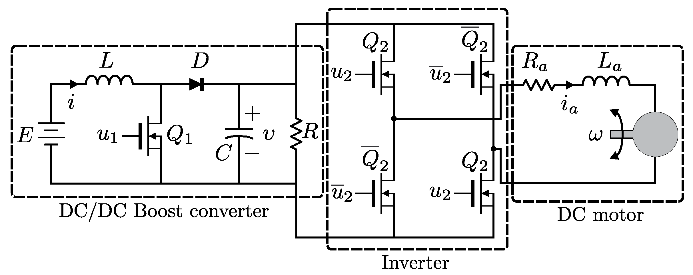
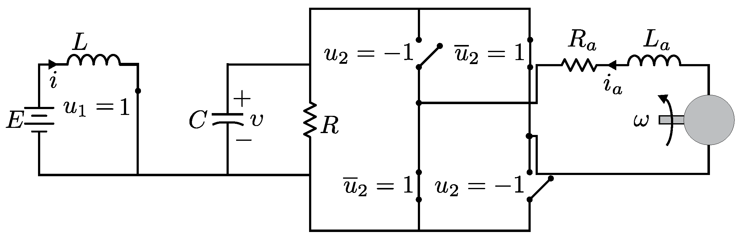
2. “DC/DC Boost Converter–Inverter–DC Motor” System

Here, the mathematical model of the DC/DC boost converter–inverter–DC motor system is developed. Additionally, the differential parametrization of the model previously deduced is presented. Such a parametrization allows the reference trajectories for the system to be generated.

2.1. Mathematical Model of the System

Figure 1 shows the electronic circuit of the DC/DC boost converter–inverter–DC motor system. This system is composed by the following:
  • DC/DC boost converter. This is composed of a power supply E, a switching input u 1 that turns on/off transistor Q 1 , a current i that flows through the inductor L, and a diode D. The output voltage, associated with capacitor C and load R, is denoted by υ .
  • Inverter. Here, u 2 and u ¯ 2 are the inputs that turn on/off transistors Q 2 and Q ¯ 2 , respectively, thus achieving the bidirectional rotation of the motor shaft.
  • DC motor. Parameters i a , R a , and L a are the armature current, armature resistance, and armature inductance; ω denotes the angular velocity of the motor shaft. Additional parameters for the DC motor are J, k e , k m , and b, which correspond to the moment of inertia of the rotor and load, the counter-electromotive force constant, the torque constant, and the viscous friction coefficient, respectively.
The ideal circuit depicted in Figure 2, which is associated with Figure 1, was used to develop the mathematical model of the system. The model was obtained by applying Kirchhoff’s current law and Kirchhoff’s voltage law to node A and mesh I (see Figure 2) and, also, by considering the mathematical model of a DC motor [37].
The operation modes of the electronic circuit shown in Figure 2 are described below. These operation modes appear when transistors are on (i.e., u 1 = 1 or u 2 = 1 ) or off (i.e., u 1 = 0 or u 2 = 1 ) generating the following four operation modes.

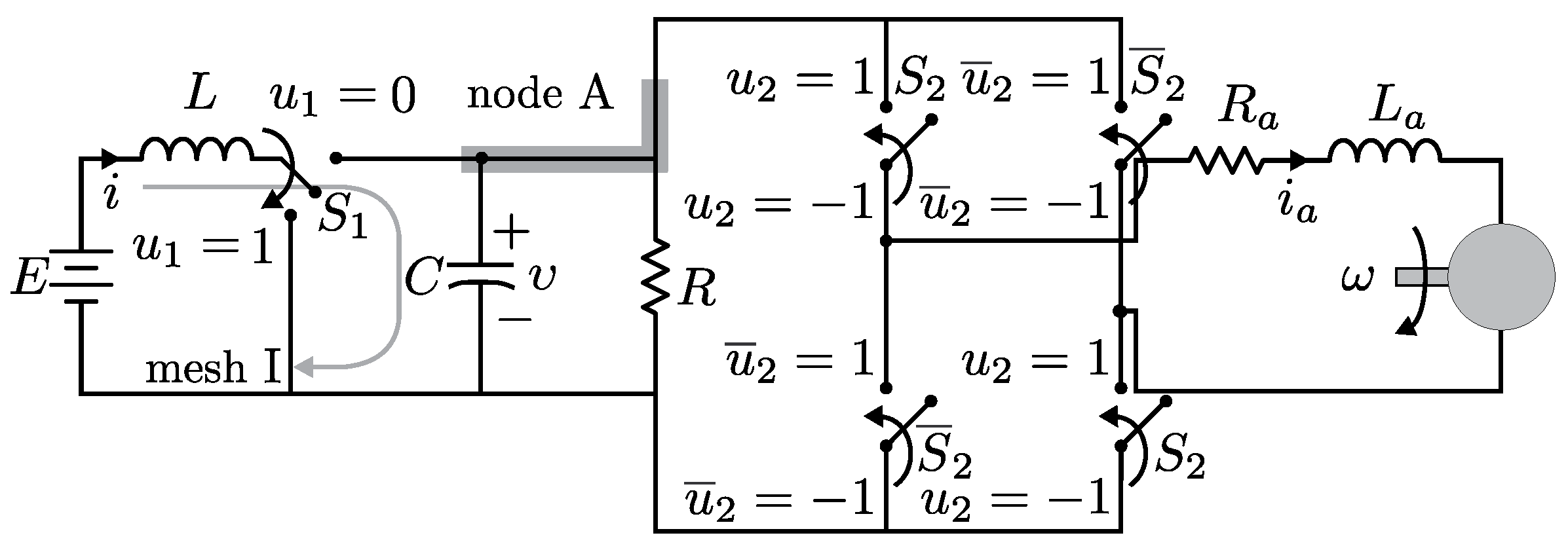
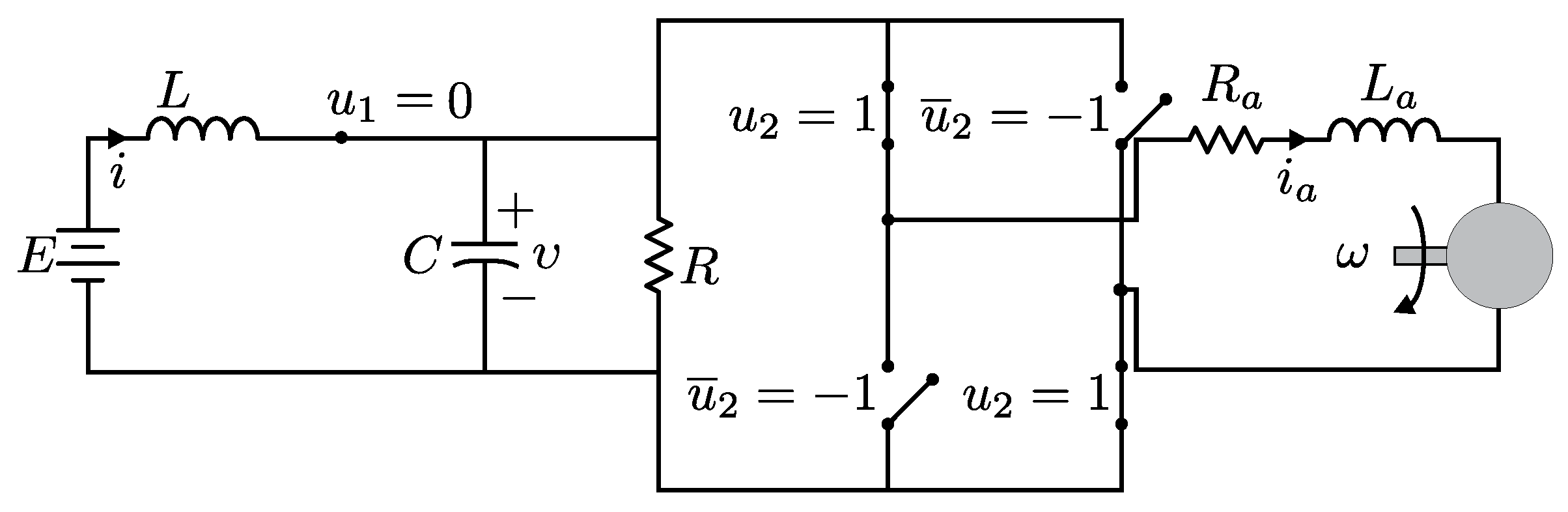
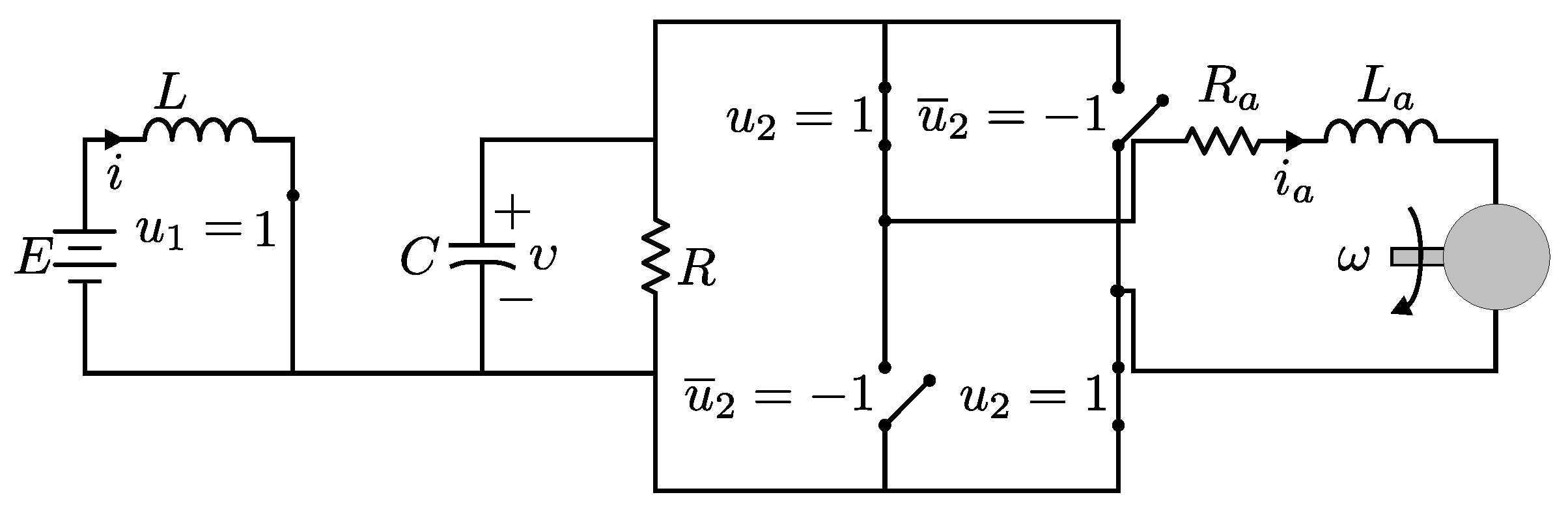
2.1.1. Operation Mode 1

Figure 3 shows the ideal electronic circuit when transistor Q 1 is off and transistor Q 2 is on, that is, u 1 = 0 and u 2 = 1 .
After applying Kirchhoff’s laws and using the mathematical model of a DC motor [37], the first operation mode is represented by the following differential equations:
L d i d t = E υ ,
C d υ d t = i υ R i a ,
L a d i a d t = υ R a i a k e ω ,
J d ω d t = k m i a b ω .

2.1.2. Operation Mode 2

This operation mode is generated when transistors Q 1 and Q 2 are off, that is, u 1 = 0 and u 2 = 1 . The equivalent circuit is depicted in Figure 4.
When Kirchhoff’s laws are applied to the circuit of Figure 4, the corresponding operation mode is modeled by
L d i d t = E υ ,
C d υ d t = i υ R + i a ,
L a d i a d t = υ R a i a k e ω ,
J d ω d t = k m i a b ω .

2.1.3. Operation Mode 3

When transistors Q 1 and Q 2 are on, that is, u 1 = 1 and u 2 = 1 , the third operation mode is generated (see Figure 5).
The mathematical model associated with this operation mode, after applying Kirchhoff’s laws, is given by
L d i d t = E ,
C d υ d t = υ R i a ,
L a d i a d t = υ R a i a k e ω ,
J d ω d t = k m i a b ω .

2.1.4. Operation Mode 4

When transistor Q 1 is on and transistor Q 2 is off, that is, u 1 = 1 and u 2 = 1 , the fourth operation mode is achieved (see Figure 6).
In this case, the operation mode is modeled by the following differential equations:
L d i d t = E ,
C d υ d t = υ R + i a ,
L a d i a d t = υ R a i a k e ω ,
J d ω d t = k m i a b ω .
After combining the four operation modes, given by Equations (1)–(16), the mathematical model of the DC/DC boost converter–inverter–DC motor system is determined by
L d i d t = ( 1 u 1 ) υ + E ,
C d υ d t = ( 1 u 1 ) i υ R i a u 2 ,
L a d i a d t = υ u 2 R a i a k e ω ,
J d ω d t = k m i a b ω ,
where u 1 and u 2 represent the switches’ positions. The mathematical model given by Equations (17)–(20) is known as the switched model because of its binary-valued nature. The average model associated with Equations (17)–(20) is as follows:
L d i d t = ( 1 u 1 a v ) υ + E ,
C d υ d t = ( 1 u 1 a v ) i υ R i a u 2 a v ,
L a d i a d t = υ u 2 a v R a i a k e ω ,
J d ω d t = k m i a b ω ,
where u 1 a v [ 0 , 1 ) and u 2 a v [ 1 , 1 ] .

2.2. Generation of Reference Trajectories

The differential parameterization of the average system given by Equations (21)–(24) is presented below.
The flat output of the boost converter, according to [38,39], is determined by its energy; that is,
E = 1 2 ( L i 2 + C υ 2 ) .
The flat output of a DC motor, according to [15], is given by the angular velocity of the motor shaft ω . After proposing the flat outputs of the DC/DC boost converter–inverter–DC motor average system as F 1 = E and F 2 = ω , the following differential parameterization associated to Equations (21)–(24) is found:
i = R C E 2 L + α ,
υ = R R C E 2 2 L + α E β i a F ˙ 1 1 / 2 ,
i a = 1 k m J F ˙ 2 + b F 2 ,
ω = F 2 ,
u 1 a v = 1 γ F ¨ 1 E 2 L 2 R 2 C υ 2 3 R C i a υ u 2 a v 1 C i a 2 u 2 a v 2 + 1 ,
u 2 a v = β υ ,
with
α = R C E 2 L 2 + 1 L C R β i a + F ˙ 1 + 2 F 1 1 / 2 , β = L a d i a d t + R a i a + k e F 2 , γ = E L υ + 2 R C i υ + 1 C i i a u 2 a v .
As can be observed, the average model given by Equations (21)–(24) is now represented by the differential parameterization given by Equations (26)–(31) expressed in terms of variables F 1 and F 2 and their corresponding derivatives with respect to time. Such a representation, compared to Equations (21)–(24), allows the reference trajectories associated with states i, υ , and i a and inputs u 1 a v and u 2 a v to be found offline [38]. Thus, when F 1 and F 2 are replaced by E * and ω * in Equations (26)–(31), the reference trajectories are obtained; this is, i * , υ * , i a * , u 1 a v * , and u 2 a v * . Here, E * is the desired boost converter energy and ω * represents the desired angular velocity of the motor shaft.

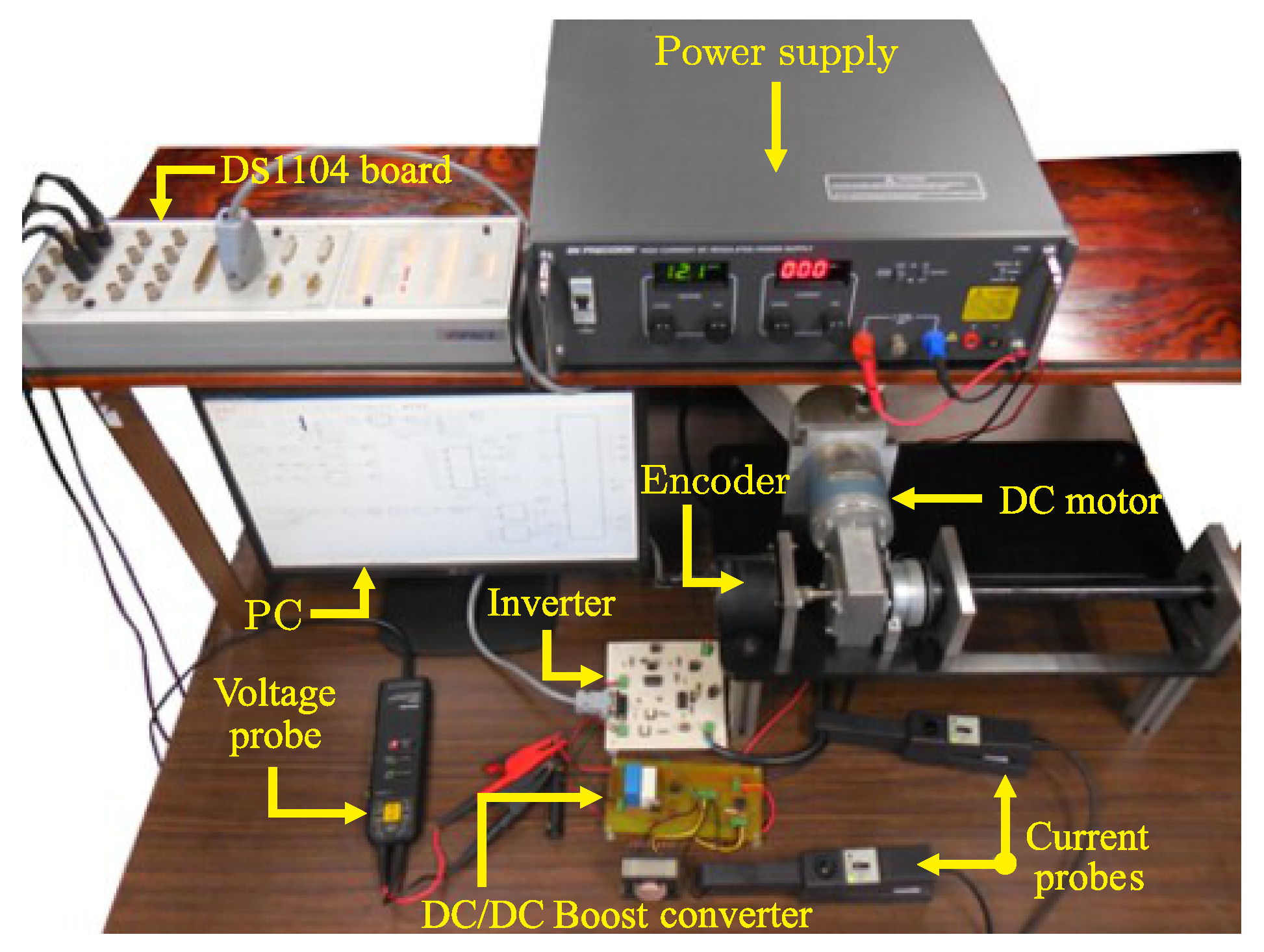
3. Built Experimental Prototype

In this section, the experimental platform used to validate the mathematical model of the boost converter–inverter–DC motor system is described.
A schematic diagram of the built platform is presented in Figure 7 and is composed of the following blocks:
  • DC/DC boost converter–inverter–DC motor system. The following three subsystems are distinguished within this block: boost converter, inverter, and DC motor. In this direction, the nominal values associated with the converter parameters are
    L = 4.94 mH , R = 64 Ω , C = 114.4 μ F , E = 12 V .
    The inverter is composed of four IRF840 MOSFET transistors driven by two IR2113 IC’s. The DC motor is an ENGEL GNM5440E-G3.1, whose nominal parameters are
    L a = 2.22 mH , k e = 120.1 × 10 3 V · s rad , R a = 0.965 Ω , k m = 120.1 × 10 3 N · m A , J = 118.2 × 10 3 kg · m 2 , b = 129.6 × 10 3 N · m · s rad .
    Similarly, variables i, i a , υ , and ω are measured via two A622 Tektronix current probes, a P5200A Tektronix voltage probe, and an E6B2-CWZ6C incremental encoder, respectively.
  • Signal conditioning and DSP. Here, the DS1104 board is electrically isolated from the power stage through the NTE3087 and TLP250 optoisolators. Additionally, this block drives the boost converter and the inverter properly by generating the switched signals u 1 and u 2 via PWM.
  • Generation of trajectories. The reference trajectories i * , υ * , i a * , u 1 a v * , and u 2 a v * and the desired trajectories E * and ω * are programmed in this block.
Figure 8 shows a picture of the built DC/DC boost converter–inverter–DC motor system. In the picture, the connections between the sensors, the DS1104 board, and the prototype can be observed.

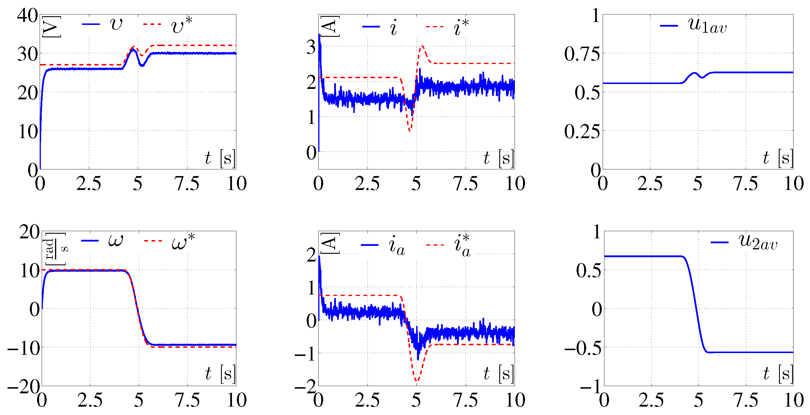
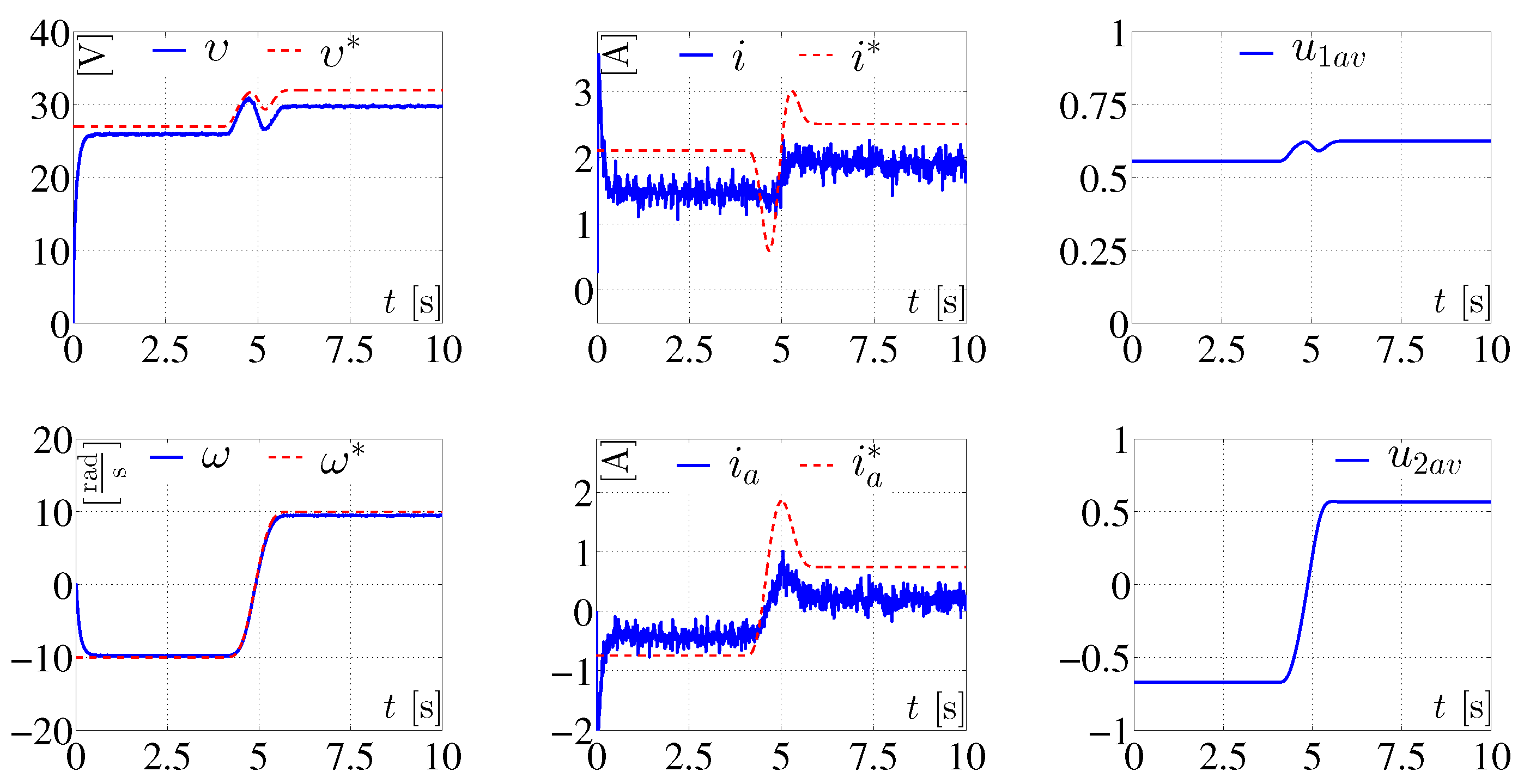
4. Experimental Results

This section presents the experimental results associated with the built prototype. Additionally, comments related to the results are included.

4.1. Experiments Performed

With the aim of verifying the mathematical model of the DC/DC boost converter–inverter–DC motor system developed in Section 2.1, five experiments are presented below.

4.1.1. Experiment 1

Here, the desired trajectories E * and ω * were determined by the following Bézier polynomials [40]:
E * ( t ) = E ¯ i ( t i ) + [ E ¯ f ( t f ) E ¯ i ( t i ) ] ψ t , t i , t f
ω * ( t ) = ω ¯ i ( t i ) + [ ω ¯ f ( t f ) ω ¯ i ( t i ) ] ψ t , t i , t f ,
where t i and t f are the initial and final times of the given trajectories. Pairs E ¯ i ( t i ) , E ¯ f ( t f ) and ω ¯ i ( t i ) , ω ¯ f ( t f ) are the constant energies and angular velocities, which are joined smoothly through E * and ω * , respectively, over the time interval t i , t f . Function ψ t , t i , t f is a polynomial defined by
ψ t , t i , t f = 0 for t t i , t t i t f t i 5 × 252 1050 t t i t f t i + 1800 t t i t f t i 2 1575 t t i t f t i 3 + 700 t t i t f t i 4 126 t t i t f t i 5 for t ( t i , t f ) , 1 for t t f .
In order to find the constant energies E ¯ i ( t i ) and E ¯ f ( t f ) , the system given by Equations (21)–(24) was considered in steady state so that i ¯ could be expressed in terms of υ ¯ and ω ¯ as follows:
i ¯ = 1 E b k m R a b k m + k e ω ¯ 2 + υ ¯ 2 R .
When Equation (34) was replaced in Equation (25), the constant energies E ¯ i ( t i ) and E ¯ f ( t f ) were obtained and were given by
E ¯ i ( t i ) = 1 2 L E 2 b k m R a b k m + k e ω ¯ i 2 + υ ¯ i 2 R 2 + 1 2 C υ ¯ i 2 ,
E ¯ f ( t f ) = 1 2 L E 2 b k m R a b k m + k e ω ¯ f 2 + υ ¯ f 2 R 2 + 1 2 C υ ¯ f 2 .
In this experiment, the constant voltages and angular velocities, υ ¯ i , υ ¯ f and ω ¯ i , ω ¯ f , associated to E * and ω * , were chosen as
υ ¯ i = 27 V , υ ¯ f = 32 V , ω ¯ i = 10 rad s , ω ¯ f = 10 rad s ,
over the time interval t i , t f = 4 s , 6 s . The experimental results are depicted in Figure 9, while the tracking errors related to variables υ , i, ω , and i a are shown in Figure 10. These tracking errors were defined as e υ = υ * υ , e i = i * i , e ω = ω * ω , and e i a = i a * i a .

4.1.2. Experiment 2

Reference trajectories E * and ω * , corresponding to the energy and the angular velocity, were defined again by Equations (32)–(33). Parameters υ ¯ i , ω ¯ i , υ ¯ f , and ω ¯ f were then selected as
υ ¯ i = 27 V , υ ¯ f = 32 V , ω ¯ i = 10 rad s , ω ¯ f = 10 rad s ,
over the same time interval t i , t f as associated with experiment 1. The corresponding results are presented in Figure 11.

4.1.3. Experiment 3

In this experiment, the desired trajectory given by Equation (32) was proposed via the following values for the constant energies E ¯ i t i and E ¯ f t f :
E ¯ i ( t i ) = 0.05 J , E ¯ f ( t f ) = 0.08 J ,
over the same time interval t i , t f as associated with experiment 1; ω * was defined as
ω * ( t ) = A sin 2 π P 1 t ( 1 e 2 t 3 ) ,
with A being the amplitude and P 1 being the period, the values of which were 10 rad s and 3 . 03 s , respectively. The experimental results are presented in Figure 12.

4.1.4. Experiment 4

The desired trajectory E * was defined as
E * ( t ) = 0.065 + 0.015 sin 2 π P 2 t ,
with P 2 = 3.03 s , while ω * was defined as in Equation (40) and parameters A and P 1 were chosen as in the previous experiment. The corresponding experimental results are plotted in Figure 13. The tracking errors related to variables υ , i, ω , and i a are depicted in Figure 14. These tracking errors were defined previously in experiment 1.

4.1.5. Experiment 5

To evaluate the dynamic behavior of the system when abrupt variations appeared in some parameters, the following change in load R was proposed:
R m = R for 0 t < 7.5 s , 30 % R for 7.5 t 10 s .
The trajectories E * and ω * considered in this experiment were given by Equations (32) and (33), and their parameters were defined by Equation (37). The experimental results are depicted in Figure 15.

4.2. Comments on the Experimental Results

Experiments 1 and 2 (Figure 9 and Figure 11). With the aim of studying the dynamic behavior of the system when constant and time-varying duty cycles are proposed (i.e., u 1 a v and u 2 a v ), experiments 1 and 2 considered E * and ω * as Bézier polynomials. Regarding υ and υ * , a small tracking error was observed in both experiments. Although currents i and i a were similar in shape to i * and i a * , respectively, their magnitudes were clearly different. With the intent of quantifying the tracking errors related to υ , i, ω , and i a of experiment 1, Figure 10 is presented. As can be observed in this figure, the errors do not converge to zero due to parasitic resistances, and energy losses were not considered in the mathematical model. Concerning experiment 2, the corresponding errors are not plotted, as the proposed trajectories were similar to those of experiment 1.
Experiments 3 and 4 (Figure 12 and Figure 13). Here, appropriate trajectories were considered for E * and ω * with the aim of generating the time-varying inputs u 1 a v and u 2 a v . It was also observed, on the one hand, that ω ω * . On the other hand, the tracking error related to voltages υ and υ * was very small, while currents i and i a were similar in shape to their reference trajectories, although their magnitudes were clearly different. The tracking errors associated with the state of experiment 4, plotted in Figure 14, again did not converge to zero for the same reason as stated in the previous paragraph. The corresponding tracking errors related to experiment 3 are not presented, as the dynamic behavior of the system was similar to that of experiment 4.
Experiment 5 (Figure 15). In this experiment, an abrupt variation was considered for load R. As a consequence, after such variation was applied to the system, signals υ and ω no longer converged to their reference signals υ * and ω * , as no control law had been designed for such a purpose.
In this manner, according to the obtained results, the experimental validation of the mathematical model presented here was satisfactory.

5. Conclusions

In this paper, the mathematical model of the DC/DC boost converter–DC motor system was developed and successfully validated. This system allows for the driving of bidirectional angular velocities. The mathematical model was obtained using circuit theory, and the experimental validation was performed on a built prototype of the system using Matlab-Simulink and a DS1104 board. The experimental tests considered time-varying duty cycles for the boost converter and the inverter by exploiting the differential flatness property of the system. Motivated by the experimental results, particularly when abrupt changes were considered in the system parameters (see Figure 15), future research will be focused on designing control techniques for solving the regulation and tracking problems related to υ and ω .

Author Contributions

Conceptualization: R.S.-O.; funding acquisition: V.H.G.-R. and H.T.; investigation: V.H.G.-R., R.S.-O., E.H.-M., J.R.G.-S., and H.T.; resources: R.S.-O.; software: V.H.G.-R., E.H.-M., and J.R.G.-S.; supervision: R.S.-O.; validation: V.H.G.-R., E.H.-M., and J.R.G.-S.; visualization: V.H.G.-R., E.H.-M., and J.R.G.-S.; writing—original draft: V.H.G.-R., R.S.-O., E.H.-M., and J.R.G.-S.; writing—review and editing: V.H.G.-R., R.S.-O., E.H.-M., J.R.G.-S., and H.T.

Acknowledgments

This work was supported by Secretaría de Investigación y Posgrado del Instituto Politécnico Nacional (SIP-IPN), México. The work of V. H. García-Rodríguez and E. Hernández-Márquez was supported by CONACYT-México and BEIFI scholarships. Additionally, V. H. García-Rodríguez and E. Hernández-Márquez acknowledge the Universidad del Istmo and the Instituto Tecnológico Superior de Poza Rica, respectively, for the ease with which they could carry out their doctoral studies at CIDETEC-IPN. Finally, R. Silva-Ortigoza and H. Taud acknowledge financial support from the IPN programs EDI and COFAA and from SNI-México.

Conflicts of Interest

The authors declare no conflict of interest.

References

  1. García-Sánchez, J.R.; Silva-Ortigoza, R.; Tavera-Mosqueda, S.; Márquez-Sánchez, C.; Hernández-Guzmán, V.M.; Antonio-Cruz, M.; Silva-Ortigoza, G.; Taud, H. Tracking control for mobile robots considering the dynamics of all their subsystems: Experimental implementation. Complexity 2017, 2017, 1–18. [Google Scholar] [CrossRef]
  2. García-Sánchez, J.R.; Tavera-Mosqueda, S.; Silva-Ortigoza, R.; Antonio-Cruz, M.; Silva-Ortigoza, G.; Rubio, J. Assessment of an avarage tracking controller that considers all the subsystems involved in a WMR: Implementation via PWM or sigma-delta modulation. IEEE Latin Am. Trans. 2016, 14, 1093–1102. [Google Scholar] [CrossRef]
  3. Silva-Ortigoza, R.; García-Sánchez, J.R.; Hernández-Guzmán, V.M.; Márquez-Sánchez, C.; Marcelino-Aranda, M. Trajectory tracking control for a differential drive wheeled mobile robot considering the dynamics related to the actuators and power stage. IEEE Latin Am. Trans. 2016, 14, 657–664. [Google Scholar] [CrossRef]
  4. Guzmán, E.; García, I.; Guerrero, E.; Pacheco, C. A tool for supporting the design of DC-DC converters through FPGA-based experiments. IEEE Latin Am. Trans. 2016, 14, 289–296. [Google Scholar] [CrossRef]
  5. Cosp, J.; Martínez, H. Design of an on-chip hybrid DC/DC converter. IEEE Latin Am. Trans. 2015, 13, 2101–2105. [Google Scholar] [CrossRef]
  6. Ortega, M.; Jurado, F.; Vera, D. Novel topology for DC-DC full-bridge unidirectional converter for renewable energies. IEEE Latin Am. Trans. 2014, 12, 1381–1388. [Google Scholar] [CrossRef]
  7. Antritter, F.; Maurer, P.; Reger, J. Flatness based control of a Buck-converter driven DC motor. In Proceedings of the 4th Symposium on Mechatronic Systems, IFAC 2006, Heidelberg, Germany, 12–14 September 2006; pp. 36–41. [Google Scholar]
  8. Lyshevski, S.E. Electromechanical Systems, Electric Machines, and Applied Mechatronics; CRC Press: Boca Raton, FL, USA, 2000; ISBN 0-8493-2275-8. [Google Scholar]
  9. Linares-Flores, J.; Reger, J.; Sira-Ramírez, H. Load torque estimation and passivity-based control of a Boost-converter/DC-motor combination. IEEE Trans. Control Syst. Technol. 2010, 18, 1398–1405. [Google Scholar] [CrossRef]
  10. Alexandridis, A.T.; Konstantopoulos, G.C. Modified PI speed controllers for series-excited DC motors fed by DC/DC Boost converters. Control Eng. Pract. 2014, 23, 14–21. [Google Scholar] [CrossRef]
  11. Konstantopoulos, G.C.; Alexandridis, A.T. Enhanced control design of simple DC-DC Boost converter-driven DC motors: Analysis and implementation. Electr. Power Compon. Syst. 2015, 43, 1946–1957. [Google Scholar] [CrossRef]
  12. Silva-Ortigoza, R.; García-Sánchez, J.R.; Alba-Martínez, J.M.; Hernández-Guzmán, V.M.; Marcelino-Aranda, M.; Taud, H.; Bautista-Quintero, R. Two-stage control design of a Buck converter/DC motor system without velocity measurements via a Σ-Δ-modulator. Math. Probl. Eng. 2013, 2013, 1–11. [Google Scholar] [CrossRef]
  13. Sira-Ramírez, H.; Oliver-Salazar, M.A. On the robust control of Buck-converter DC-motor combinations. IEEE Trans. Power Electron. 2013, 28, 3912–3922. [Google Scholar] [CrossRef]
  14. Silva-Ortigoza, R.; Márquez-Sánchez, C.; Carrizosa-Corral, F.; Antonio-Cruz, M.; Alba-Martínez, J.M.; Saldaña-González, G. Hierarchical velocity control based on differential flatness for a DC/DC Buck converter-DC motor system. Math. Probl. Eng. 2014, 2014, 1–12. [Google Scholar] [CrossRef]
  15. Silva-Ortigoza, R.; Hernández-Guzmán, V.M.; Antonio-Cruz, M.; Muñoz-Carrillo, D. DC/DC Buck power converter as a smooth starter for a DC motor based on a hierarchical control. IEEE Trans. Power Electron. 2015, 30, 1076–1084. [Google Scholar] [CrossRef]
  16. Hernández-Guzmán, V.M.; Silva-Ortigoza, R.; Muñoz-Carrillo, D. Velocity control of a brushed DC–motor driven by a DC to DC Buck power converter. Int. J. Innov. Comp. Inf. Control 2015, 11, 509–521. Available online: http://www.ijicic.org/ijicic-14-04031.pdf (accessed on 10 June 2018).
  17. Kumar, S.G.; Thilagar, S.H. Sensorless load torque estimation and passivity based control of Buck converter fed DC motor. Sci. World J. 2015, 2015, 1–15. [Google Scholar] [CrossRef] [PubMed]
  18. Khubalkar, S.; Chopade, A.; Junghare, A.; Aware, M.; Das, S. Design and realization of stand-alone digital fractional order PID controller for Buck converter fed DC motor. Circuits Syst. Signal Process. 2016, 35, 2189–2211. [Google Scholar] [CrossRef]
  19. Rigatos, G.; Siano, P.; Wira, P.; Sayed-Mouchaweh, M. Control of DC-DC converter and DC motor dynamics using differential flatness theory. Intell. Ind. Syst. 2016, 2, 371–380. [Google Scholar] [CrossRef]
  20. Nizami, T.K.; Chakravarty, A.; Mahanta, C. Design and implementation of a neuro-adaptive backstepping controller for Buck converter fed PMDC-motor. Control Eng. Pract. 2017, 58, 78–87. [Google Scholar] [CrossRef]
  21. Chakravarty, A.; Nizami, T.K.; Mahanta, C. Real time implementation of an adaptive backstepping control of Buck converter PMDC-motor combinations. In Proceedings of the Indian Control Conference, Guwahati, India, 4–6 January 2017; pp. 277–282. [Google Scholar]
  22. Roy, T.K.; Paul, L.C.; Sarkar, M.I.; Pervej, M.F.; Tumpa, F.K. Adaptive controller design for speed control of DC motors driven by a DC-DC Buck converter. In Proceedings of the International Conference on Electrical, Computer and Communication Engineering, Cox’s Bazar, Bangladesh, 16–18 February 2017; pp. 100–105. [Google Scholar]
  23. Ahmad, M.A.; Raja-Ismail, R.M.T. A data-driven sigmoid-based PI controller for Buck-converter powered DC motor. In Proceedings of the IEEE Symposium on Computer Applications and Industrial Electronics, Langkawi Island, Malaysia, 24–25 April 2017; pp. 81–86. [Google Scholar]
  24. Nizami, T.K.; Chakravarty, A.; Mahanta, C. A fast learning neuro adaptive control of Buck converter driven PMDC-motor: Design, analysis and validation. In Proceedings of the 20th IFAC World Congress, Toulouse, France, 9–14 July 2017; pp. 37–42. [Google Scholar]
  25. Wu, H.; Zhang, L.; Yang, J.; Li, S. Model predictive control for DC-DC Buck power converter-DC motor system with uncertainties using GPI observer. In Proceedings of the 36th Chinese Control Conference, Dalian, China, 26–28 July 2017; pp. 4906–4911. [Google Scholar]
  26. Sönmez, Y.; Dursun, M.; Güvenç, U.; Yilmaz, C. Start up current control of Buck-Boost convertor-fed serial DC motor. Pamukkale Univ. J. Eng. Sci. 2009, 15, 278–283. Available online: https://www.journalagent.com/pajes/pdfs/PAJES_15_2_278_283.pdf (accessed on 10 June 2018).
  27. Linares-Flores, J.; Barahona-Avalos, J.L.; Sira-Ramírez, H.; Contreras-Ordaz, M.A. Robust passivity-based control of a Buck-Boost-converter/DC–motor system: An active disturbance rejection approach. IEEE Trans. Ind. Appl. 2012, 48, 2362–2371. [Google Scholar] [CrossRef]
  28. Jiménez-Toribio, E.E.; Labour-Castro, A.A.; Muñiz-Rodríguez, F.; Pérez-Hernández, H.R.; Ortiz-Rivera, E.I. Sensorless control of Sepic and Ćuk converters for DC motors using solar panels. In Proceedings of the IEEE International Electric Machines and Drives Conference (IEMDC 2009), Miami, FL, USA, 3–6 May 2009; pp. 1503–1510. [Google Scholar]
  29. Silva-Ortigoza, R.; Alba-Juárez, J.N.; García-Sánchez, J.R.; Antonio-Cruz, M.; Hernández-Guzmán, V.M.; Taud, H. Modeling and Experimental Validation of a Bidirectional DC/DC Buck Power Electronic Converter-DC Motor System. IEEE Latin Am. Trans. 2017, 15, 1043–1051. [Google Scholar] [CrossRef]
  30. Silva-Ortigoza, R.; Alba-Juárez, J.N.; García-Sánchez, J.R.; Hernández-Guzmán, V.M.; Sosa-Cervantes, C.Y.; Taud, H. A sensorless passivity-based control for the DC/DC Buck converter–inverter–DC motor system. IEEE Latin Am. Trans. 2016, 14, 4227–4234. [Google Scholar] [CrossRef]
  31. Hernández-Márquez, E.; García-Sánchez, J.R.; Silva-Ortigoza, R.; Antonio-Cruz, M.; Hernández-Guzmán, V.M.; Taud, H.; Marcelino-Aranda, M. Bidirectional tracking robust controls for a DC/DC Buck converter-DC motor system. Complexity 2017, in press. [Google Scholar]
  32. García-Rodríguez, V.H.; Silva-Ortigoza, R.; Hernández-Márquez, E.; García-Sánchez, J.R.; Ponce-Silva, M.; Saldaña-González, G. A DC motor driven by a DC/DC Boost converter-inverter: Modeling and simulation. In Proceedings of the 2016 International Conference on Mechatronics, Electronics and Automotive Engineering, ICMEAE 2016, Cuernavaca, Morelos, Mexico, 22–25 November 2016; pp. 78–83. [Google Scholar]
  33. García-Rodríguez, V.H.; García-Sánchez, J.R.; Silva-Ortigoza, R.; Hernández-Márquez, E.; Taud, H.; Ponce-Silva, M.; Saldaña-González, G. Passivity based control for the Boost converter-inverter- DC motor system. In Proceedings of the 2017 International Conference on Mechatronics, Electronics and Automotive Engineering, ICMEAE 2017, Cuernavaca, Morelos, Mexico, 21–24 November 2017; pp. 77–81. [Google Scholar]
  34. Hernández-Márquez, E.; Silva-Ortigoza, R.; García-Sánchez, J.R.; García-Rodríguez, V.H.; Alba-Juárez, J.N. A new DC/DC Buck-Boost converter–DC motor system: Modeling and experimental validation. IEEE Latin Am. Trans. 2017, 15, 2043–2049. [Google Scholar] [CrossRef]
  35. Hernández-Márquez, E.; Silva-Ortigoza, R.; García-Sánchez, J.R.; Marcelino-Aranda, M.; Saldaña-González, G. A DC/DC Buck-Boost converter-inverter-DC motor system: Sensorless passivity-based control. IEEE Access 2018, 6, 31486–31492. [Google Scholar] [CrossRef]
  36. Linares-Flores, J.; Sira-Ramírez, H.; Cuevas-López, E.F.; Contreras-Ordaz, M.A. Sensorless passivity based control of a DC motor via a solar powered Sepic converter-full bridge combination. J. Power Electron. 2011, 11, 743–750. [Google Scholar] [CrossRef]
  37. Hernández-Guzmán, V.M.; Silva-Ortigoza, R.; Carrillo-Serrano, R.V. Control Automático: Teoría de Diseño, Construcción de Prototipos, Modelado, Identificación y Pruebas Experimentales; Colección CIDETEC-IPN: Mexico City, Mexico, 2013; ISBN 978-607-414-362-1. [Google Scholar]
  38. Sira-Ramírez, H.; Silva-Ortigoza, R. Control Design Techniques in Power Electronics Devices; Springer-Verlag: London, UK, 2006; ISBN 978-1-84628-458-8. [Google Scholar]
  39. Silva-Ortigoza, R.; Sira-Ramírez, H.; Hernández-Guzmán, V.M. Control por modos deslizantes y planitud diferencial de un convertidor de CD/CD Boost: Resultados experimentales. Rev. Iberoam. Autom. Inform. Ind. 2008, 5, 77–82. [Google Scholar] [CrossRef]
  40. Biagiotti, L.; Melchiorri, C. Trajectory Planning for Automatic Machines and Robots; Springer-Verlag: London, UK, 2008; ISBN 978-3-540-85628-3. [Google Scholar]
Figure 1. DC/DC boost converter–inverter–DC motor system.
Energies 11 02044 g001
Figure 2. Ideal circuit of DC/DC boost converter–inverter–DC motor system.
Energies 11 02044 g002
Figure 3. Equivalent circuit when u 1 = 0 and u 2 = 1 .
Energies 11 02044 g003
Figure 4. Equivalent circuit when u 1 = 0 and u 2 = 1 .
Energies 11 02044 g004
Figure 5. Equivalent circuit when u 1 = 1 and u 2 = 1 .
Energies 11 02044 g005
Figure 6. Equivalent circuit when u 1 = 1 and u 2 = 1 .
Energies 11 02044 g006
Figure 7. Block diagram of the built experimental prototype.
Energies 11 02044 g007
Figure 8. Built experimental prototype.
Energies 11 02044 g008
Figure 9. System response for Equations (32)–(33) and parameters given by Equations (37).
Energies 11 02044 g009
Figure 10. Tracking errors related to experiment 1.
Energies 11 02044 g010
Figure 11. System response for Equations (32)–(33) and parameters given by Equation (38).
Energies 11 02044 g011
Figure 12. System response for Equations (32) and (40).
Energies 11 02044 g012
Figure 13. System response for Equations (40) and (41).
Energies 11 02044 g013
Figure 14. Tracking errors related to experiment 4.
Energies 11 02044 g014
Figure 15. System response for Equations (32)–(33), parameters given by Equation (37), and abrupt variation in load R.
Energies 11 02044 g015

