Numerical Investigation of the Effects of Steam Mole Fraction and the Inlet Velocity of Reforming Reactants on an Industrial-Scale Steam Methane Reformer

Department of Aeronautical Engineering, National Formosa University, Huwei, Yunlin 632, Taiwan
Energies 2018, 11(8), 2082; https://doi.org/10.3390/en11082082
Submission received: 1 July 2018
/
Revised: 3 August 2018
/
Accepted: 8 August 2018
/
Published: 10 August 2018
(This article belongs to the Special Issue Cleaner Combustion)
Abstract
:Steam methane reforming (SMR) is the most common commercial method of industrial hydrogen production. Control of the catalyst tube temperature is a fundamental demand of the reformer design because the tube temperature must be maintained within a range that the catalysts have high activity and the tube has minor damage. In this paper, the transport and chemical reaction in an industrial-scale steam methane reformer are simulated using computational fluid dynamics (CFD). Two factors influencing the reformer temperature, hydrogen yield and stress distribution are discussed: (1) the mole fraction of steam (YH2O) and (2) the inlet velocity of the reforming reactants. The purpose of this paper is to get a better understanding of the flow and thermal development in a reformer and thus, to make it possible to improve the performance and lifetime of a steam reformer. It is found that the lowest temperature at the reforming tube surface occurs when YH2O is 0.5. Hydrogen yield has the highest value when YH2O is 0.5. The wall shear stress at the reforming tube surface is higher at a higher YH2O. The surface temperature of a reforming tube increases with the inlet velocity of the reforming reactants. Finally, the wall shear stress at the reforming tube surface increases with the inlet velocity of the reforming reactants.
1. Introduction
The environmental impact of greenhouse gas pollutants emitted from the combustion of fossil fuels and the legal regulations against production of air pollutants have increased the necessity for clean combustion. Hydrogen is an efficient energy carrier and is one of the cleanest fuels which can replace fossil fuels. Hydrogen is also an important material for petroleum refineries. It converts crude oil into products with high economic value, e.g., gasoline, jet fuel and diesel. The demand for hydrogen by petroleum refineries has increased due to environmental restrictions and efforts to process heavier components of crude oil. In particular, the environmental requirement for low-sulfur-content fuels results in an increasing amount of hydrogen required in hydro-treating processes, and the attempt to process heavier components of crude oil, known as bottom-of-the-barrel processing, also increases the demand for hydrogen in hydro-cracking processes [1,2,3].
A wide and generalized use of hydrogen would be feasible only when efficient means of producing it with low emission of pollutants were industrially developed. Hydrogen can be produced by a number of ways, e.g., electrolysis, steam methane reforming (SMR), partial oxidation reforming, nuclear energy, etc. [4,5]. Among these ways, SMR is the most common commercial method of industrial hydrogen production. SMR reaction mainly includes the following three chemical equations:
CH4 + H2O ⇄ CO + 3H2
CO + H2O ⇄ CO2 + H2
CH4 + 2H2O ⇄ CO2 + 4H2
The first (SMR) and the third reactions are endothermic, the second reaction (water-gas shift (WGS)) is exothermic, and the overall reaction is endothermic.
A steam reformer of a hydrogen plant is a device that supplies heat to convert the natural gas or liquid petroleum gas into hydrogen via catalysts. The combustion process in a reformer provides heat to maintain the reforming reaction in a catalyst tube. Control of the catalyst tube temperature is a fundamental demand of the reformer design because the tube temperature must be maintained within a range that the catalysts have high activity and the tube has minor damage. When a steam reformer is operating, the catalyst tubes are subjected to stresses close to the ultimate stress of the tube material. This leads to an acceleration of the creep damage. Safety, reliability and efficiency are the basic requirements of the reformer operation. The catalyst tube should have uniform heat distribution to extend tube life. However, the heat distribution in a reformer is practically non-uniform. In addition, maldistribution of the flue gas and fuel gas may result in flame impingement on the catalyst tubes and lead to localized hot spots and high tube wall temperature. These factors may shorten the tube life.
Owing to the rapid development in computer science and technology, as well as the improvements in physical models and numerical methods, computational fluid dynamics (CFD) is widely used in analyzing systems involving heat transfer, fluid flow and chemical reactions. CFD is also used to simulate systems that cannot be measured easily or simulated experimentally. In recent years, there have been a lot of SMR researches using CFD. Tran et al. [1] developed a CFD model of an industrial-scale steam methane reformer. The authors pointed out that the reformer CFD model can be considered an adequate representation of the on-line reformer and can be used to determine the risk of operating the online reformer at unexplored and potentially more beneficial operating conditions. Di Carlo et al. [2] investigated numerically a pilot scale bubbling fluidized bed SE-SMR (Sorption Enhanced Steam Methane Reforming) reactor by means of a two-dimensional CFD approach. The numerical results show quantitatively the positive influence of carbon dioxide sorption on the reforming process at different operating conditions, specifically the enhancement of hydrogen yield and reduction of methane residual concentration in the reactor outlet stream. Lao et al. [6] developed a CFD model of an industrial-scale reforming tube using ANSYS Fluent with realistic geometry characteristics to simulate the transport and chemical reaction phenomena with approximate representation of the catalyst packing. The authors analyzed the real-time regulation of the hydrogen production by choosing the outer wall temperature profile of the reforming tube and the hydrogen concentration at the outlet as the manipulated input and controlled output, respectively. Mokheimer et al. [7] presented modeling and simulations of SMR process. The model was applied to study the effect of different operating parameters on the steam and methane conversion. The results showed that increasing the conversion thermodynamic limits with the decrease of the pressure results in a need for long reformers so as to achieve the associated fuel reforming thermodynamics limit. It is also shown that not only increasing the steam to methane molar ratio is favorable for higher methane conversion but the way the ratio is changed also matters to a considerable extent. Ni [8] developed a 2D heat and mass transfer model to investigate the fundamental transport phenomenon and chemical reaction kinetics in a compact reformer for hydrogen production by SMR. Parametric simulations were performed to examine the effects of permeability, gas velocity, temperature, and rate of heat supply on the reformer performance. It was found that the reaction rates of SMR and WGS are the highest at the inlet but decrease significantly along the reformer. Increasing the operating temperature raises the reaction rates at the inlet but shows very small influence downstream. Ebrahimi et al. [9] applied a three-dimensional zone method to an industrial fired heater of SMR reactor. The effect of emissivity, extinction coefficient, heat release pattern and flame angle on performance of the fired heater are presented. It was found that decreasing the extinction coefficients of combustion gases by 25% caused 2.6% rise in the temperature of heat sink surfaces. Seo et al. [10] investigated numerically a compact SMR system integrated with a WGS reactor. Heat transfer to the catalyst beds and the catalytic reactions in the SMR and WGS catalyst beds were investigated. The effects of the cooling heat flux at the outside wall of the system and steam-to-carbon ratio were also examined. It was found that as the cooling heat flux increases, both the methane conversion and carbon monoxide content are reduced in the SMR bed and the carbon monoxide conversion is improved in the WGS bed. In addition, both methane conversion and carbon dioxide reduction increase with increasing steam-to-carbon ratio.
In this paper, the transport and chemical reaction in an industrial-scale steam methane reformer are simulated using CFD. Two factors influencing the reformer temperature, hydrogen yield and stress are discussed. They include the mole fraction of steam and the inlet velocity of the reforming reactants. The objective is to get a better understanding of the flow and thermal development in a reformer and thus to make it possible to improve the performance and lifetime of a steam reformer.
2. Numerical Methods and Physical Models
In this study, the ANSYS FLUENT V.17 commercial code [11] is employed to simulate the reacting and fluid flow in a steam methane reformer. The SIMPLE algorithm by Patankar [12] is used to solve the governing equations. The discretizations of convection terms and diffusion terms are carried out by the second order upwind scheme and the central difference scheme, respectively. In respect to physical models, by considering the accuracy and stability of the models and by referring to the other CFD researches [1,2,6] of steam methane reformers, the standard k-ε model [13], discrete ordinate (DO) radiation model [14] and finite rate/eddy dissipation (FRED) model [15] are adopted for turbulence, radiation and chemical reaction simulations, respectively. The standard wall functions [16] are used to resolve the flow quantities (velocity, temperature, and turbulence quantities) at the near-wall regions.
For the steady-state three-dimensional flow field with chemical reaction in this study, the governing equations include the continuity equation, momentum equation, turbulence model equation (k-ε model), energy equation, radiation model equation (discrete ordinate radiation model), and chemical reaction model equation (FRED model). Among these models, only the FRED chemical reaction model is described below while the others and the convergence criterion are not described because they have been introduced in the author’s previous study [17].
Consider the general form of the rth chemical reaction as follows:
where
- N = number of chemical species in the system
- = stoichiometric coefficient for reactant i in reaction r
- = stoichiometric coefficient for product i in reaction r
- μi = species i
- = forward rate constant for reaction r
- = backward rate constant for reaction r
Equation (4) is valid for both reversible and non-reversible reactions. For non-reversible reactions, the backward rate constant, kb,r, is omitted. The species transport equation of a chemical reaction system can be written as
where Yi, Di,m, Sct, Ri, and Si are the mass fraction, diffusion coefficient, turbulent Schmidt number, net generation rate, and extra source term of species i, respectively. The net source of chemical species i due to reaction is computed as the sum of the Arrhenius reaction sources over the NR reactions that the species participate in
where Mw,i is the molecular weight of species i and is the Arrhenius molar rate of creation/destruction of species i in reaction r. For a non-reversible reaction, the molar rate of creation/destruction of species i in reaction r is given by
For a reversible reaction,
where
- = molar concentration of species j in reaction r (kgmol/m3)
- = rate exponent for reactant species j in reaction r
- = rate exponent for product species j in reaction r
- Γ = net effect of third bodies on the reaction rate
The forward and backward rate constants for reaction r, kf,r and kb,r, are computed using the Arrhenius expression:
where
kf,r = ArTβre−Er/RT
- Ar = pre-exponential factor (consistent units)
- βr = temperature exponent (dimensionless)
- Er = activation energy for the reaction (J/kgmol)
- R = universal gas constant (J/kgmol-K)
Kr is the equilibrium constant for the rth reaction and is computed from
where patm denotes atmospheric pressure (101, 325 Pa). The term within the exponential function represents the change in Gibbs free energy, and its components are computed as follows:
where Sio and hio are the standard-state entropy and standard-state enthalpy (heat of formation). In this study, the kinetic and thermodynamic constants for reactions (1)–(3) used in Lemnouer Chibane and Brahim Djellouli’s work [18] are adopted.
In general, a reformer operates at high temperatures. For a non-premixed reaction, turbulence mixes the reactants and then advects the mixture to the reaction zone for quick reaction. For a premixed reaction, turbulence mixes the lower-temperature reactants and the higher-temperature products and then advects the mixture to the reaction zone for a quick reaction. Therefore, the chemical reaction is generally mixing (diffusion) controlled. However, the flue gas, fuel gas and air are generally premixed before injecting into the reformer. Although the chemical reaction in most regions in a reformer is mixing controlled, in some regions, e.g., the neighborhood of the feed inlet, the chemical reaction is kinetically controlled. In existing chemical reaction models, the eddy dissipation model (EDM) [19] can consider simultaneously the diffusion controlled and the kinetically controlled reaction rates. In EDM, the net generation rate of species i in the rth chemical reaction is found from the smaller value of the following two reaction rates:
where
- Yp is the mass fraction of any product, P
- YR is the mass fraction of a particular reactant, R
- A is an empirical constant equal to 4.0
- B is an empirical constant equal to 0.5
In general, the EDM works well for a non-premixed reaction. However, for a premixed reaction, the reaction may start immediately when injecting into a reformer. This is unrealistic in practical situations. To overcome this unreasonable phenomenon, ANSYS FLUENT provides another model, the Finite-Rate/Eddy-Dissipation (FRED) model, which combines the finite-rate model and the EDM. In this model, the net generation rate of a species is taken as the smaller value of the Arrhenius reaction rate and the value determined by EDM. The Arrhenius reaction rate plays the role of a switch to avoid the unreasonable situation that the reaction starts immediately when injecting into a reformer. Once the reaction is activated, the eddy-dissipation rate is generally lower than the Arrhenius reaction rate, and the reaction rate is then determined by the EDM.
3. Results and Discussion
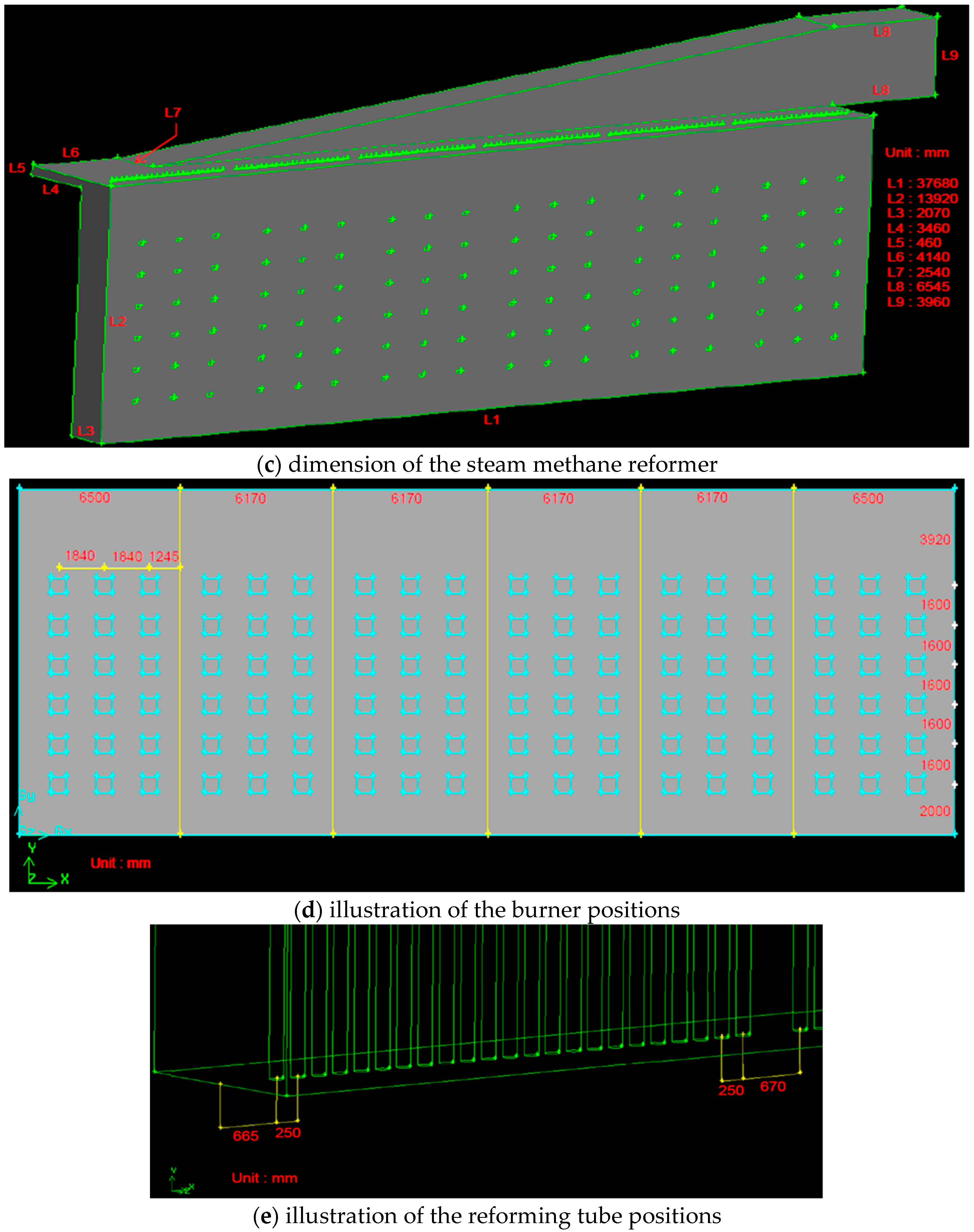
To validate the numerical methods and physical models used in this study, an industrial-scale steam methane reformer is simulated. The configuration and dimension of the reformer investigated is shown in Figure 1. Note that only one half of the reformer is simulated due to its symmetry, as shown in Figure 1b,c. The reformer contains 138 reforming tubes and 216 burners on one side (totally 276 tubes and 432 burners). The outer diameter and thickness of a reforming tube are 136 mm and 13.4 mm, respectively, while the diameter of a burner is 197 mm.
The boundary conditions for the numerical model of the steam methane reformer are described below. These conditions are practical operating conditions that are used by a petrochemical corporation in Taiwan.
- (1)
- Symmetry plane: symmetric boundary condition
- (2)
- Wall: standard wall function
- (3)
- Reforming tube inlet:
- V = 5.4 m/s (in axial direction)
- T = 912.75 K
- Pgauge = 2.1658 × 10⁶ N/m2
Species mole fraction:- CH4 = 0.2029
- H2O = 0.6
- H2 = 0.12855
- CO2 = 0.06565
- CO = 0.00145
- N2 = 0.00145
- (4)
- Reforming tube exit:The diffusion flux for all flow variables in the outflow direction are zero. In addition, the mass conservation is obeyed at the exit.
- (5)
- Fuel and flue gas inlet (burner inlet):
- V = 2.404 m/s (in radial direction)
- T = 673.15 K
- Pgauge = 1.04544 × 10⁴ N/m2
Species mole fraction:- H2 = 0.0816
- CH4 = 0.0474
- N2 = 0.49057
- O2 = 0.12818
- CO2 = 0.25225
- (6)
- Fuel and flue gas exit:The diffusion flux for all flow variables in the outflow direction are zero. In addition, the mass conservation is obeyed at the exit.
The turbulence kinetic energy is 10% of the inlet mean flow kinetic energy and the turbulence dissipation rate is computed using Equation (16).
where l = 0.07 L and L is the hydraulic diameter.
3.1. Comparison of Numerical Results with Experimental Data
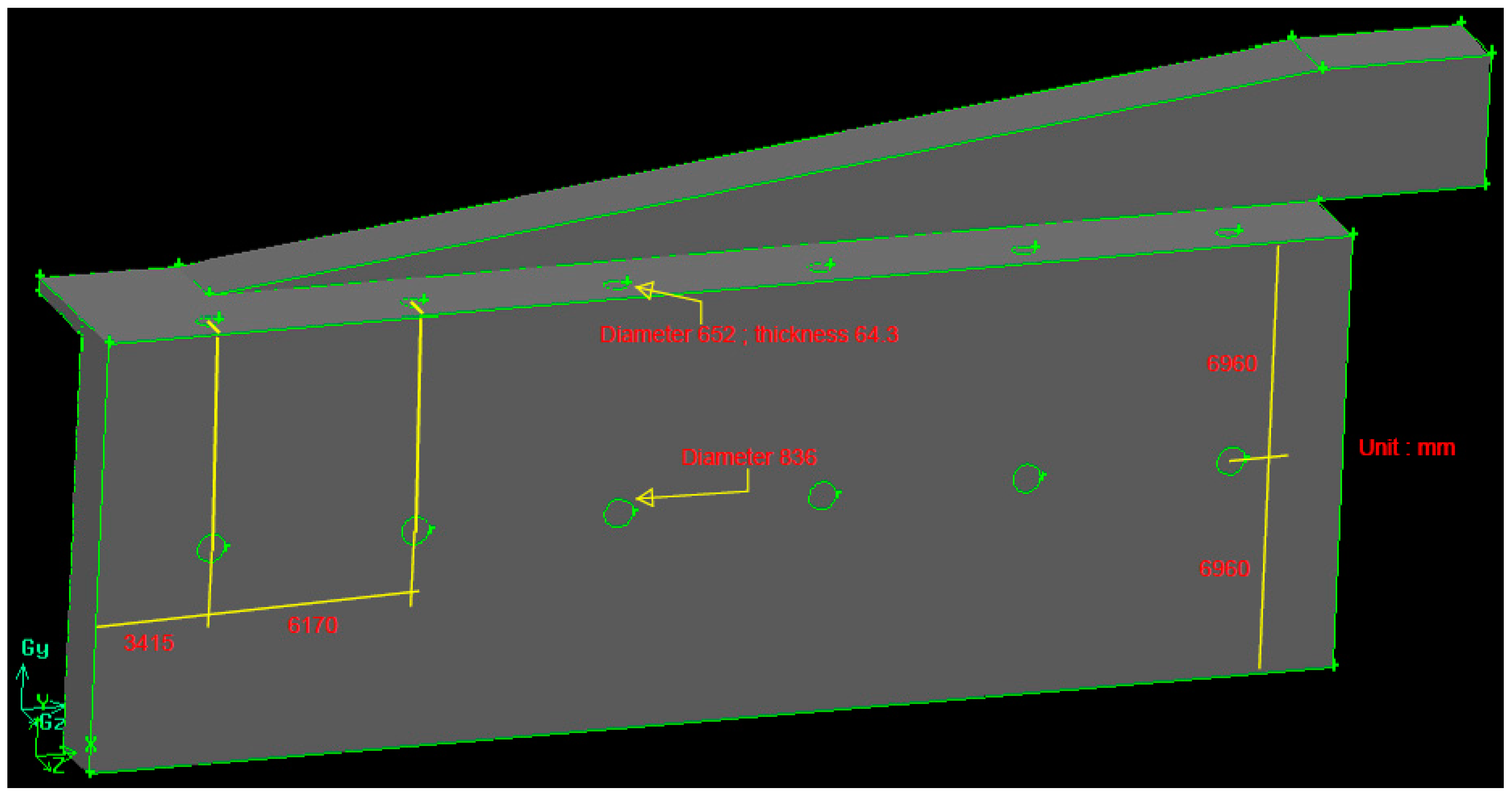
The simulation results are compared with the experimental data from a petrochemical refinery in Taiwan to evaluate the numerical methods and physical models adopted in this study. As mentioned above, the real reformer contains 138 reforming tubes and 216 burners on one side (totally 276 tubes and 432 burners). To save simulation time, a simplified model is also calculated and compared. The simplified model contains 6 tubes and 12 burners on one side of the reformer. The arrangement of reforming tubes and burners as well as their dimensions for the simplified model are shown in Figure 2. The flowrates in the reforming tubes and burners for the simplified model are the same as those in the real reformer. Therefore, the reforming tubes and burners for the simplified model have larger diameters.
The numbers of CFD cells for the real reformer model and the simplified model are around 4 million and 1.5 million, respectively. The grid mesh is generated by the software GAMBIT and is unstructured. The dimensionless distance from the wall, y*, in the wall function method has been examined after a converged solution is obtained. It was found that the values of y* for the nodes at the wall to their nearest interior nodes vary between 20.0 and 60.0, and lie in the logarithmic layer of the wall function method. This implies that the wall-adjacent cells of the grid mesh in this study are suitable for the use of wall function.
The computer used in this study is an ASUS ESC-500-G4 work station of 8 cores with Intel Core i7-6700 CPU and 64 GB ram. The solution of the CFD model for the real reformer is obtained after approximately 30 full days while that for the simplified reformer is approximately 10 full days.
Figure 3 compares the average temperatures at the outer surfaces of the reforming tubes. It can be seen that the simulation result agrees well with the experimental data. The deviations from the experimental data using the real reformer model and the simplified model are 2.88% and 3.18%, respectively, which are both acceptable from a viewpoint of engineering applications. The result calculated from the real reformer model agrees better with the experimental data than that from the simplified model, although the latter also gives an acceptable result.
In the subsequent discussion, the simplified model is used for parametric study to save simulation time.
3.2. Effect of the Mole Fraction of Steam
To explore the effect of steam quantities used in the SMR process on the hydrogen yield, seven different mole fractions of steam (YH2O), 0.1, 0.2, 0.3, 0.4, 0.5, 0.6, and 0.7 are calculated and compared. The mole fraction of steam for practical operation is 0.6. The mole fractions of the other species in the reforming reactants, except methane, are kept unchanged. This implies that the mole fraction of methane decreases when the mole fraction of steam increases.
Figure 4 compares the average temperatures at the surfaces of the reforming tubes using different mole fractions of steam. From the simulation results, the lowest average temperatures at the surfaces (outer or inner) of the reforming tubes occur when YH2O is 0.5. The reforming reactants with a steam mole fraction of 0.5 are approximately a stoichiometric mixture, which has a more complete reforming reaction. From Figure 4, it is also observed that the inner surface temperature of the reforming tube is lower than its outer surface temperature at this inlet velocity of reforming reactants (5.4 m/s). The effect of inlet velocities of the reforming reactants will be discussed in the next section.
The above result can also be observed from Figure 5 which compares the average mole fractions of hydrogen at the reforming tube outlets using different mole fractions of steam. As expected, the hydrogen yield has the highest value when YH2O is 0.5 because of a more complete reforming reaction. When YH2O is less than 0.5, the hydrogen yield increases with YH2O. On the other hand, when YH2O is greater than 0.5, the hydrogen yield decreases with YH2O. Further, it can be found from Figure 5 that the simulated hydrogen yield is 0.708 for the steam mole fraction of real operation (i.e., YH2O = 0.6). The real value of the hydrogen yield is 0.698. The deviation of the CFD simulation is 1.43%
When a steam reformer is operating, the catalyst tubes are subjected to stresses close to the ultimate stress of the tube material. This leads to an acceleration of the creep damage. Figure 6 compares the average wall shear stresses at the surfaces of the reforming tubes using different mole fractions of steam. It can be observed that higher wall shear stresses at the surfaces of the reforming tubes occur at higher YH2O. For example, the highest wall shear stress at the surfaces of the reforming tubes occurs when YH2O is 0.7. From Figure 6, it is also observed that the wall shear stresses at the inner surfaces of the reforming tubes are higher than those at their outer surfaces.
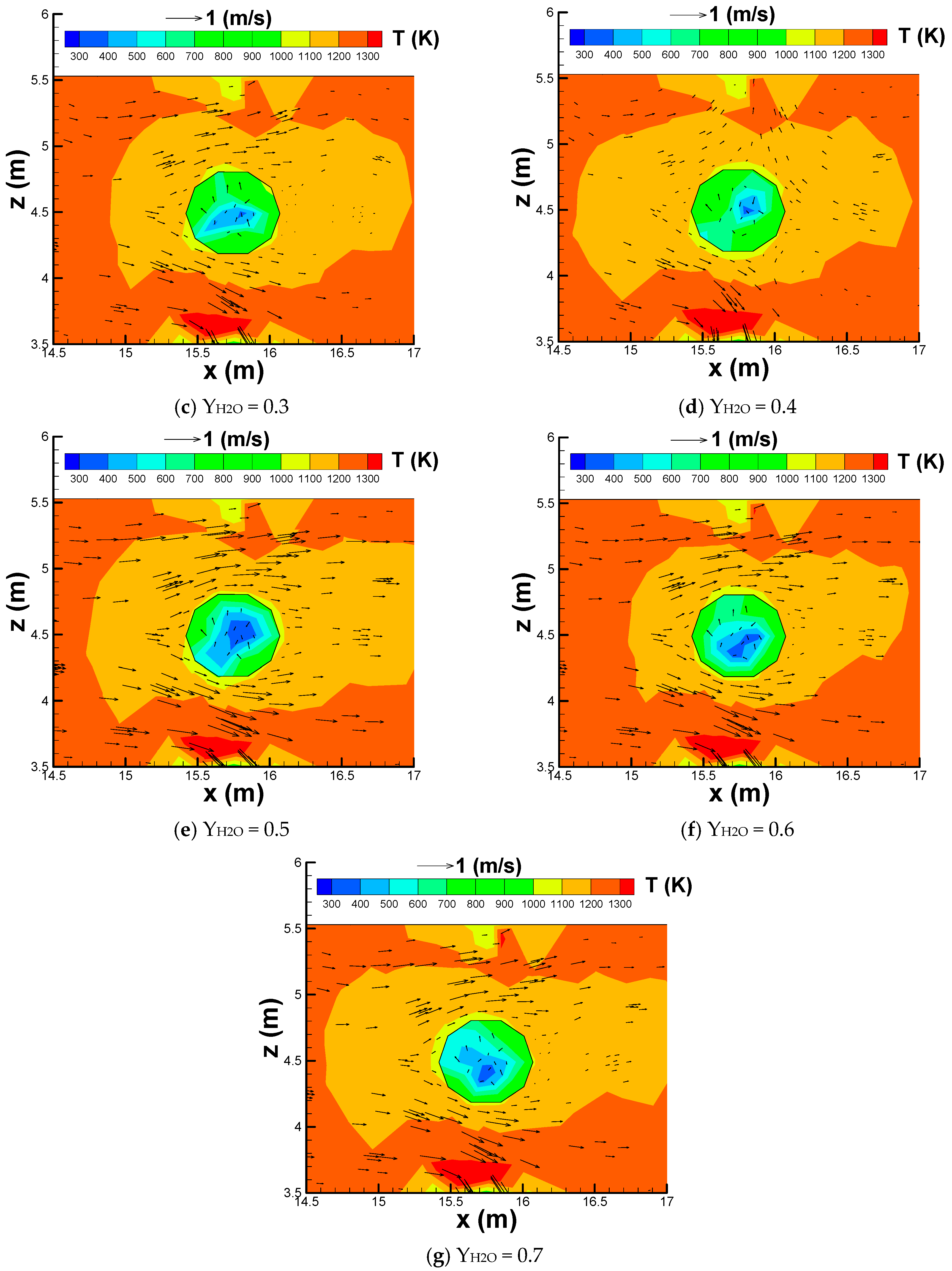
To explore the influence of the flow and thermal development on the wall shear stress, Figure 7 compares the temperature and velocity vector distributions at y = 6 m around a reforming tube using different mole fractions of steam. It is observed that the wall shear stress is closely connected with the velocity vector distributions around the reforming tube. A faster flow through a reforming tube results in a higher wall shear stress.
3.3. Effect of Inlet Velocities of the Reforming Reactants
To explore the effect of inlet velocities of the reforming reactants on hydrogen yield, five different inlet velocities of the reforming reactants (Vreforming reactants), 1.35, 2.7, 5.4, 8.1 and 10.8 m/s are calculated and compared. The inlet velocity of reforming reactants for the real operation is 5.4 m/s. The mole fraction of steam in the reforming reactants is taken as 0.5 because it is close to a stoichiometric mixture, which has a more complete reforming reaction. The other operating conditions, including pressure, temperature, velocity, and species composition, on the burner side and reforming tube side are kept unchanged.
Figure 8 compares the average temperatures at the surfaces of the reforming tubes using different inlet velocities of the reforming reactants. It is observed that the surface temperatures (outer and inner) of the reforming tubes increase with the inlet velocities of the reforming reactants. It should be noted that the tolerance of temperature for a reforming tube is around 950 °C. Therefore, the inlet velocity of the reforming reactants should not exceed the real value 5.4 m/s too much. When the inlet velocities of the reforming reactants are lower, the outer surface temperatures of the reforming tubes are higher than their inner surface temperatures. On the other hand, when the inlet velocities of the reforming reactants are higher, the inner surface temperatures of the reforming tubes are higher than their outer surface temperatures. From Figure 8, it is also observed that the inner surface temperatures of the reforming tubes are more sensitive to the inlet velocities of the reforming reactants, as compared to their outer surface temperatures.
Figure 9 compares the average mole fractions of hydrogen at the reforming tube outlets using different inlet velocities of the reforming reactants. Because the mole fractions of the reforming reactants are kept unchanged, it is observed that the inlet velocity of the reforming reactants has a minor influence on the hydrogen yields at the reforming tube outlets. However, because the flowrate of the reforming reactants is proportional to their inlet velocity, the hydrogen yields are naturally increased when the inlet velocity of the reforming reactants is increased.
Figure 10 compares the average wall shear stresses at the surfaces of the reforming tubes using different inlet velocities of the reforming reactants. It is observed that the wall shear stresses at the surfaces of the reforming tubes increase with the inlet velocity of the reforming reactants. Similar to the results using different mole fractions of steam, the wall shear stresses at the inner surfaces of the reforming tubes are higher than those at their outer surfaces. To explore the influence of the flow and thermal development on the wall shear stress, Figure 11 shows the comparison of the temperature and velocity vector distributions at y = 6 m around a reforming tube using different inlet velocities of the reforming reactants. Similar to the results using different mole fractions of steam, it is found that the wall shear stress is closely connected with the velocity vector distributions around a reforming tube. A faster fluid flow through a reforming tube results in a larger wall shear stress. From Figure 11 it is also observed that the temperature inside and outside a reforming tube increases with the inlet velocity of the reforming reactants. The overall reaction inside a reforming tube is endothermic. Increasing the velocity of the reforming reactants also increases the reforming tube temperatures due to the higher heat absorption of the reforming reactants. This also increases the temperature outside the reforming tubes due to the radiation emission from the reforming tubes. The tolerance of the reforming tube temperature, 950 °C, may be exceeded. Therefore, it should be careful when using higher velocities of the reforming reactants to increase the hydrogen production. The inlet velocity of the reforming reactants should not exceed the real value (5.4 m/s) too much.
4. Conclusions
In this paper, the transport and chemical reaction in an industrial-scale steam methane reformer are simulated using CFD. Two factors influencing the reformer temperature, hydrogen yield and stress distribution are discussed: (1) the mole fraction of steam and (2) the inlet velocity of reforming reactants. The purpose of this paper is to get a better understanding of the flow and thermal development in a steam reformer and thus, to make it possible to improve the performance and lifetime of a steam reformer. From the simulation results, it is found that the lowest temperature at the reforming tube surfaces occurs when YH2O is 0.5. Hydrogen yield has the highest value when YH2O is 0.5. Hydrogen yield increases with YH2O when YH2O is less than 0.5 and decreases with YH2O when YH2O is greater than 0.5. The wall shear stress at a reforming tube surface is higher at a higher YH2O. A faster fluid flow through a reforming tube results in a larger wall shear stress. The surface temperature of a reforming tube increases when the inlet velocity of the reforming reactants increases. When the inlet velocity of the reforming reactants is lower, the outer surface temperature of a reforming tube is higher than its inner surface temperature. On the other hand, when the inlet velocity of the reforming reactants is higher, the inner surface temperature of a reforming tube is higher than its outer surface temperature. As compared to the outer surface temperature of a reforming tube, its inner surface temperature is more sensitive to the inlet velocity of the reforming reactants. Finally, the wall shear stress at a reforming tube surface increases when the inlet velocity of the reforming reactants increases.
Funding
This research and the APC were funded by the Ministry of Science and Technology, Taiwan, under the contract MOST106-2221-E-150-061.
Acknowledgments
The author is grateful to the Formosa Petrochemical Corporation in Taiwan for providing valuable data and constructive suggestions to this research during the execution of the industry-university cooperative research project under the contract 104AF-86.
Conflicts of Interest
The author declares no conflict of interest.
Abbreviations
The following abbreviations are used in this manuscript:
| Cμ | turbulence model constant (=0.09) |
| K | turbulence kinetic energy (m2/s2) |
| P | pressure (N/m2) |
| T | temperature (K) |
| V | velocity (m/s) |
| XYZ | cartesian coordinates with origin at the centroid of the burner inlet (m) |
| Y | mole fraction (%) |
| Greek symbols | |
| ε | turbulence dissipation rate (m2/s3) |
| μ | viscosity (kg/(m s)) |
| ρ | density (kg/m3) |
| τ | shear stress (N/m2) |
References
- Tran, A.; Aguirre, A.; Durand, H.; Crose, M.; Christofides, P.D. CFD modeling of an industrial-scale steam methane reforming furnace. Chem. Eng. Sci. 2017, 171, 576–598. [Google Scholar] [CrossRef]
- Di Carlo, A.; Aloisi, I.; Jand, N.; Stendardo, S.; Foscolo, P.U. Sorption enhanced steam methane reforming on catalyst-sorbent bifunctional particles: A CFD fluidized bed reactor model. Chem. Eng. Sci. 2017, 173, 428–442. [Google Scholar] [CrossRef]
- Irani, M.; Alizadehdakhel, A.; Nakhaei Pour, A.; Hoseini, N.; Adinehnia, M. CFD modeling of hydrogen production using steam reforming of methane in monolith reactors: Surface or volume-base reaction model? Int. J. Hydrogen Energy 2011, 36, 15602–15610. [Google Scholar] [CrossRef]
- Kimmel, A.S. Heat and Mass Transfer Correlations for Steam Methane Reforming in Non-Adiabatic, Process-Intensified Catalytic Reactors. Master’s Thesis, Marquette University, Milwaukee, WI, USA, 2011. [Google Scholar]
- Castagnola, L.; Lomonaco, G.; Marotta, R. Nuclear systems for hydrogen production: State of art and perspectives in transport sector. Glob. J. Energy Technol. Res. Updat. 2014, 1, 4–18. [Google Scholar]
- Lao, L.; Aguirre, A.; Tran, A.; Wu, Z.; Durand, H.; Christofides, P.D. CFD modeling and control of a steam methane reforming reactor. Chem. Eng. Sci. 2016, 148, 78–92. [Google Scholar] [CrossRef] [Green Version]
- Mokheimer, E.M.A.; Hussain, M.I.; Ahmed, S.; Habib, M.A.; Al-Qutub, A.A. On the modeling of steam methane reforming. J. Energy Resour. Technol. 2015, 137, 012001. [Google Scholar] [CrossRef]
- Ni, M. 2D heat and mass transfer modeling of methane steam reforming for hydrogen production in a compact reformer. Energy Convers. Manag. 2013, 65, 155–163. [Google Scholar] [CrossRef] [Green Version]
- Ebrahimi, H.; Soltan Mohammadzadeh, J.S.; Zamaniyan, A.; Shayegh, F. Effect of design parameters on performance of a top fired natural gas reformer. Appl. Therm. Eng. 2008, 28, 2203–2211. [Google Scholar] [CrossRef]
- Seo, Y.-S.; Seo, D.-J.; Seo, Y.-T.; Yoon, W.-L. Investigation of the characteristics of a compact steam reformer integrated with a water-gas shift reactor. J. Power Sources 2006, 161, 1208–1216. [Google Scholar] [CrossRef]
- Fluent Inc. ANSYS FLUENT 17 User’s Guide; Fluent Inc.: New York, NY, USA, 2017. [Google Scholar]
- Patankar, S.V. Numerical Heat Transfer and Fluid Flows; McGraw-Hill: New York, NY, USA, 1980. [Google Scholar]
- Launder, B.E.; Spalding, D.B. Lectures in Mathematical Models of Turbulence; Academic Press: London, UK, 1972. [Google Scholar]
- Siegel, R.; Howell, J.R. Thermal Radiation Heat Transfer; Hemisphere Publishing Corporation: Washington, DC, USA, 1992. [Google Scholar]
- Sivathanu, Y.R.; Faeth, G.M. Generalized state relationships for scalar properties in non-premixed hydrocarbon/air flames. Combust. Flame 1990, 82, 211–230. [Google Scholar] [CrossRef]
- Launder, B.E.; Spalding, D.B. The numerical computation of turbulent flows. Comput. Method Appl. Mech. 1974, 3, 269–289. [Google Scholar] [CrossRef]
- Yeh, C.L. Numerical analysis of the combustion and fluid flow in a carbon monoxide boiler. Int. J. Heat Mass Transf. 2013, 59, 172–190. [Google Scholar] [CrossRef]
- Chibane, L.; Djellouli, B. Methane steam reforming reaction behaviour in a packed bed membrane reactor. Int. J. Chem. Eng. Appl. 2011, 2, 147–156. [Google Scholar] [CrossRef]
- Magnussen, B.F.; Hjertager, B.H. On mathematical models of turbulent combustion with special emphasis on soot formation and combustion. In Symposium (international) on Combustion; The Combustion Institute: Pittsburgh, PA, USA, 1976. [Google Scholar]
Figure 1.
Configuration and dimension of the steam methane reformer investigated.


Figure 2.
The arrangement of reforming tubes and burners as well as their dimensions for the simplified model.
Figure 2.
The arrangement of reforming tubes and burners as well as their dimensions for the simplified model.

Figure 3.
Comparison of the average temperatures at the outer surfaces of the reforming tubes.

Figure 4.
Comparison of the average temperatures at the surfaces of the reforming tubes using different mole fractions of steam.
Figure 4.
Comparison of the average temperatures at the surfaces of the reforming tubes using different mole fractions of steam.

Figure 5.
Comparison of the average mole fractions of hydrogen at the reforming tube outlets using different mole fractions of steam.
Figure 5.
Comparison of the average mole fractions of hydrogen at the reforming tube outlets using different mole fractions of steam.

Figure 6.
Comparison of the average wall shear stresses at the surfaces of the reforming tubes using different mole fractions of steam.
Figure 6.
Comparison of the average wall shear stresses at the surfaces of the reforming tubes using different mole fractions of steam.

Figure 7.
Comparison of the temperature and velocity vector distributions at y = 6 m around a reforming tube using different mole fractions of steam.
Figure 7.
Comparison of the temperature and velocity vector distributions at y = 6 m around a reforming tube using different mole fractions of steam.


Figure 8.
Comparison of the average temperatures at the surfaces of the reforming tubes using different inlet velocities of the reforming reactants.
Figure 8.
Comparison of the average temperatures at the surfaces of the reforming tubes using different inlet velocities of the reforming reactants.

Figure 9.
Comparison of the average mole fractions of hydrogen at the reforming tube outlets using different inlet velocities of the reforming reactants.
Figure 9.
Comparison of the average mole fractions of hydrogen at the reforming tube outlets using different inlet velocities of the reforming reactants.

Figure 10.
Comparison of the average wall shear stresses at the surfaces of the reforming tubes using different inlet velocities of the reforming reactants.
Figure 10.
Comparison of the average wall shear stresses at the surfaces of the reforming tubes using different inlet velocities of the reforming reactants.

Figure 11.
Comparison of the temperature and velocity vector distributions at y = 6 m around a reforming tube using different inlet velocities of the reforming reactants.
Figure 11.
Comparison of the temperature and velocity vector distributions at y = 6 m around a reforming tube using different inlet velocities of the reforming reactants.


© 2018 by the author. Licensee MDPI, Basel, Switzerland. This article is an open access article distributed under the terms and conditions of the Creative Commons Attribution (CC BY) license (http://creativecommons.org/licenses/by/4.0/).
Share and Cite
MDPI and ACS Style
Yeh, C.-L. Numerical Investigation of the Effects of Steam Mole Fraction and the Inlet Velocity of Reforming Reactants on an Industrial-Scale Steam Methane Reformer. Energies 2018, 11, 2082. https://doi.org/10.3390/en11082082
AMA Style
Yeh C-L. Numerical Investigation of the Effects of Steam Mole Fraction and the Inlet Velocity of Reforming Reactants on an Industrial-Scale Steam Methane Reformer. Energies. 2018; 11(8):2082. https://doi.org/10.3390/en11082082
Chicago/Turabian StyleYeh, Chun-Lang. 2018. "Numerical Investigation of the Effects of Steam Mole Fraction and the Inlet Velocity of Reforming Reactants on an Industrial-Scale Steam Methane Reformer" Energies 11, no. 8: 2082. https://doi.org/10.3390/en11082082
Note that from the first issue of 2016, this journal uses article numbers instead of page numbers. See further details here.