Cross-Border Effects on Swiss Electricity Prices in the Light of the Energy Transition

Abstract

Given the perspective of the Swiss energy policy to support investments in renewable energy sources, it becomes highly relevant at this point to understand cross-border effects of imported electricity on the Swiss electricity prices. We found that German (Phelix) and Swiss (Swissix) electricity prices are cointegrated, given that the two markets are interconnected. We examined the cross-border effects of the German market fundamentals on Swissix, taking into account seasonality aspects. In the context of a dynamic fundamental model, we found that there is a continuous adaption process of electricity prices to market fundamentals and that this effect depends on the season of the year and the time of the day. Model results reveal the substitution effect between traditional fuels and renewable energies due to their alternative use in production and the shift in the merit order curve. Results are of great relevance to Swiss policy makers: Switzerland imports lower electricity prices due to the energy transition in Germany. In particular, because of the high infeed of PV (photovoltaic) during peak hours, the spread between Swissix peak and off-peak prices narrowed significantly over time. Incentives for investments in renewable energies in Switzerland as well as subsidies for hydropower should be considered in the light of these insights.

1. Introduction

In this paper, we identify the fundamental market factors that impact Swiss electricity wholesale prices (Swissix), given the interconnector between the German and Swiss power markets. Given the perspective of the Swiss energy policy to support investments in new installations of wind and PV (photovoltaic), as well as in flexible storage devices (see, for example, [1] or [2]), an understanding of the fundamental factors that impact Swiss electricity prices becomes highly relevant. In particular, we emphasize the seasonal profile of imports of renewable energies and focus on their interchange in production with traditional sources (coal, gas, oil).

Liberalised markets are typically characterized by more market competition, higher economic efficiencies and lower prices. Altogether, its result is a higher total welfare, which is also the aim of the European Electricity Market. The first steps of the liberalisation process were implemented in December 1996 by means of the EU Directive 96/92/EC [3]. The main objective of this directive was to increase competition and to regulate existing monopolies. Switzerland also reacted in the mid-1990s and started to draft a law called “Electricity Market Law” (German: Elektrizitätsmarktgesetz, EMG), whose purpose was the market liberalisation within six years and the development of a national private-law grid company [4].

The EMG was rejected in 2002, whereupon the Swiss Federal Council embedded the stepwise liberalisation in the “Power Supply Law” (Stromversorgungsgesetz, StromVG). The latter was passed in 2007, and in preparation of its implementation the Transmission System Operator (TSO) Swissgrid was already established one year earlier. The law became effective in 2008 and allowed large consumers to choose their power supplier freely from January 2009 on. Five years later, the market should have been opened for all consumers, but, because of the Fukushima nuclear disaster, the Energy Strategy 2050 had to be revised and, therefore, the full liberalisation in Switzerland was postponed.

It is important to distinguish between the regulatory opening of the market and the physical interconnections within the countries. The electricity grids of 36 countries in Europe are already physically interconnected, including Switzerland. The grid operators of these countries are organized in the European Network of Transmission System Operators for Electricity (ENTSO-E).

The liberalisation of power markets enables, in addition, energy trading across international borders, but, due to limited physical capacities of the transmission lines at the borders, price differences across countries still remain. These prices are strongly influenced by the capacity auctioning mechanism in the different countries involved. Parallel to this contractual layer, the increasing importance of sustainable environment management led to an expansion of fluctuant renewable power infeed, especially in Germany (see [5]).

Renewable energy infeed in Germany is proven to have a high impact on the day-ahead electricity price in Austria and Germany [6]. Furthermore, the intraday trading activities to adjust energy production- and consumption forecasts have increased significantly over the last years, partially because of the high share of fluctuating renewable power which needs to be balanced out [7]. As these technologies have extremely low variable costs and their production is fed into the grid with priority, they cause a shift in the merit order curve, which results in lower electricity prices [8]. This development influences the traditional relation between fossil fuel prices and electricity prices since coal, gas or oil are partially substituted by renewable energies in the production mix [6].

The introduction of market coupling in many European countries initiated also a price shift, as a striking convergence of electricity prices took place among the countries participating in this process [9]. Switzerland is not yet included in the market coupling mechanism between Germany, Austria and France, but the German and the Swiss markets are interconnected and cross-border effects are expected to occur. At the border between Switzerland and Germany, implicit capacity allocations have been used since June 2013: the capacity auction is implicitly embedded in the electricity auction. The price that is paid therefore reflects both the price for the electricity and for the congestion on high voltage lines. This mechanism ensures an efficient energy flow from the low price area with a surplus of energy to the high price area.

Figure 1 shows the net cross-border electricity exchange, namely Swiss imports of electricity from Germany minus exports, on average per week between 2009 and 2016. We observe that, in winter months, when water storage for hydropower is getting empty and the thawing period has not yet started, Switzerland imports electricity from Germany, which sets upwards pressure on Swissix prices with a larger spread to Phelix). In summer, when the country is able to export energy produced by hydropower, prices are typically lower. The cross-border exchange of electricity between Switzerland and Germany is reflected in the evolution of electricity prices in the two countries.

Empirical evidence shows that Swiss electricity prices are mainly determined by German Phelix prices [8]. This can be seen from the reaction of the Swissix on 15 January 2015, when the Swiss National Bank unpegged the Franc from the Euro, and Swissix prices, which are quoted in EUR/MWh, did not react to this policy change (see Figure 2). The market interconnectedness of the Swiss, German and Austrian power market prevents that Swiss power producers, who have costs in Swiss Francs, enforce higher prices for electricity traded in the now weaker Euro. In fact, it also has been shown empirically that prices are cointegrated. Additionally, it has also been shown that Swissix prices are Granger-caused by Phelix. It is therefore important to disentangle the marginal effects of the German market fundamentals on Swiss wholesale prices.

Paraschiv, Erni and Pietsch [6] show that there is a continuous price adaption effect of Phelix prices to traditional market fundamentals: coal, gas, oil, CO${}_2$ prices, demand and power plant availability. Furthermore, Ref. [10] shows that this effect varies across price quantiles. The price adaption comes from two sources: adaption of electricity prices to input fuel prices and substitution/replacement in production of traditional fuels (in particular gas and oil) by renewable energies, i.e., wind and PV (photovoltaic). Renewable energies substituted the more expensive technologies in production and, thus, decreased electricity prices due to the merit order effect.

The precondition for Switzerland for a participation in the market coupling mechanism is the conclusion of the already drafted bilateral agreement on electricity with the European Union, which has been suspended. In the light of the current status of Switzerland and with the perspective of a future introduction of market coupling, an investigation of the impact of fundamental factors for electricity prices in the neighbouring countries on Swiss power prices is highly relevant. Our analysis will refer to cross-border effects of German fundamental factors on Swissix prices.

The rest of the paper is organized as follows: in Section 2, we describe the data that were identified as fundamental drivers for power prices, namely prices of traditional (fossil) fuels and emission certificates, infeed from renewable energies, demand and power plant availability. Section 3 provides empirical evidence for the joint dynamics of Swissix and Phelix prices and attests to the existence of cross-border effects. The dependency of Swiss electricity prices to fundamental variables with an impact on power prices in the neighbour country Germany is analysed further in Section 4 by means of a regression model with time-varying coefficients estimated by a Kalman filter. Section 5 discusses the results and their economic interpretation. The last Section 6 summarises the main findings and their relevance for policy makers.

2. Data

Traditionally, electricity production in Germany was mainly based on nuclear power, coal, gas and oil. Over the last few years, supported by governmental subsidies, there has been a continuous growth in the penetration of wind and PV sources (see

Table 1. Electricity production in Germany by source (%), see [12].

	2009	2010	2011	2012	2013	2014	2015	2016
Coal	42.5	41.5	42.8	44.0	45.1	43.7	42.0	40.2
Nuclear	22.6	22.2	17.6	15.8	15.2	15.5	14.2	13.0
Natural Gas	13.6	14.1	14.0	12.1	10.6	9.7	9.8	12.5
Oil	1.7	1.4	1.2	1.2	1.1	0.9	1.0	0.9
Renewable Energies from which	16.0	16.5	20.2	22.8	23.8	25.8	29.1	29.2
Wind	6.6	6.1	8.1	8.2	8.2	9.3	12.4	12.3
Hydro Power	3.2	3.3	2.9	3.5	3.6	3.1	2.9	3.2
Biomass	4.4	4.6	5.2	6.1	6.3	6.7	6.9	6.9
Photovoltaic	1.1	1.8	3.2	4.2	4.9	5.7	6.0	5.9
Waste-to-Energy	0.7	0.7	0.8	0.8	0.8	1.0	0.9	0.9
Other	3.6	4.2	4.2	4.1	4.1	4.3	4.1	4.2

). Typically, the most expensive technology on use sets the electricity price, which varies within a day. Switzerland imports from Germany both (fossil) fuel-based and renewable electricity.

In our analysis, we model cross-border effects on day-ahead Swiss electricity prices of market fundamentals that traditionally impact the neighbouring power market in Germany. We take into account both demand and supply-side factors: expected demand, expected power plant availability as well as prices for coal, gas and oil. Data are ex-ante information for the electricity day-ahead price formation mechanism, i.e., the last observations before the day-ahead electricity price auction at the European Power Exchange (EPEX) [9]. In addition, we take into account the latest available information of expected wind and PV infeed in Germany before the electricity price is formed. Ex-ante weather data are retrieved and aggregated from Transmission System Operators.

The daily seasonality pattern of prices is taken into account by deriving one individual model for each hour of the day. The weekly and yearly seasonality is incorporated in the expected demand variable. It is well known that the cyclical pattern of electricity prices is highly correlated with the demand, which is inflexible. In [11], the authors investigate the load demand flexibility and findings show that each consumer incurs a discomfort cost by changing its load demand from the desired pattern to the scheduled pattern. In this way, we distinguish between different load levels, where power plants with different marginal costs of production are on use. Typically, in hours with a low level of demand (night hours), the power production in Germany is mainly coal-based, while, during peak hours, the excess demand (The demand that is not yet covered by the infeed from renewable energies (wind and PV)) is covered by more expensive plants like gas and oil.

In addition, we include the lagged electricity market clearing price for the same hour of the previous relevant delivery day and the price of the same hour with the lag of one week. This helps to reduce autocorrelation in our data and, furthermore, incorporates historical price and risk signals, which usually influence agents’ price expectations and risk aversion.

The rationale behind choosing these fundamental variables is given in detail in Section 3.1 (“Price Formation Fundamentals”) of the study by [10] for the market area Germany/Austria. The data set spans from 1 January 2011 to 31 August 2016. We give a detailed overview of the sources and granularity of the relevant data in

Table 2. Overview of fundamental variables.

Variable Units	Description	Data Source
Lag Spot Price (1 day) Swissix in EUR/MWh	Market clearing price for the same hour of the previous relevant delivery day	European Energy Exchange: https://www.epexspot.com/de/
Lag Spot Price (7 days) Swissix in EUR/MWh	Market clearing price for the same hour of the same weekday in the previous week	European Energy Exchange: https://www.epexspot.com/de/
Coal Price EUR/t	Latest available price (daily auctioned) of the front-month Amsterdam–Rotterdam–Antwerp (ARA) futures contract before the electricity price auction takes place	European Energy Exchange: https://www.epexspot.com/de/
Gas Price EUR/MWh	Last price of the NCG (NetConnect Germany) Day Ahead Natural Gas Spot Price on the day before the electricity price auction takes place	Bloomberg, Ticker: EGTHDAHD Index
Oil Price EUR/bbl	Last price of the active Brent Crude futures contract at the Intercontinental Exchange (ICE) on the day before the electricity price auction takes place	Bloomberg, Ticker: CO1 Comdty
Price for EUA EUR/EUA	Latest available price of the daily EUA auctions at the European Energy Exchange (EEX) Emission Market	European Energy Exchange: http://www.eex.com
Expected Wind and Photovoltaic Infeed MW	Sum of expected infeed of wind electricity into the grid, published by German transmission system operators in the late afternoon following the electricity price auction	Transmission system operators: http://www.50Hertz.com, http://www.amprion.de, http://www.transnetbw.de, http://www.tennettso.de
Expected Power Plant Availability MW	Ex-ante expected power plant availability for electricity production (voluntary publication) on the delivery day (daily granularity), daily published at 10:00 a.m.	European Energy Exchange & transmission system operators: ftp://infoproducts.eex.com
Expected Demand MW	Sum of total vertical system load and actual wind infeed for the same hour on the last relevant delivery day	Transmission system operators: http://www.50Hertz.com, http://www.amprion.de, http://www.transnetbw.de, http://www.tennettso.de

and

Table 3. Data granularity of fundamental variables.

Variable	Code	Daily	Hourly
Lag Spot Price (1 day)	LagSpot1day		×
Lag Spot Price (7 days)	LagSpot7days		×
Coal Price	CoalPr	×
Gas Price	GasPr	×
Oil Price	OilPr	×
Price for EU Emission Allowances	CO${}_2$Pr	×
Expected Wind	ExpWind		×
Expected Photovoltaic Infeed	ExpPV		×
Expected Power Plant Availability	ExpPPA	×
Expected Demand	ExpDemand		×

Note: × marks if daily or hourly data are available for the corresponding variable and used in the estimation.

.

3. Preliminary Analysis

A theoretical background for the cross-border effects between Switzerland and Germany was given in detail in Section 1. Figure 1 confirms the link between the electricity exchange between the two markets and its direct effect on prices. In this section, we provide statistical evidence to prove the joint dynamics between Swissix and Phelix prices and, furthermore, to prove that the variables which traditionally impact German electricity prices have cross-border significant marginal effects on Swissix prices. We analyse here the statistical link between Swissix and Phelix and perform a linear regression between Swissix and fundamental variables presented in Table 2.

All variables presented in Table 2 are tested for stationarity. Swissix and Phelix are stationary time series. However, the prices of fuels (coal, gas, oil) and EUA (European Union Allowance) emission certificates are non-stationary, which must be taken into account in the estimation approach. Augmented Dickey–Fuller test results are available upon request.

We first check for the statistical relation between the two electricity price indexes, Swissix and Phelix. As explained in the Introduction, and confirmed by previous empirical evidence [8], Swiss electricity prices are mainly determined by German Phelix prices, given that Switzerland is a net importer of German power almost over the entire year as illustrated in Figure 1. Equation (1) gives us the long-term co-movement between the two price series.

Table 4. Linear regression between Swissix and Phelix price series.

Dependent Variable: SWISSIX
Variable	Coefficient	Standard Error
C	13.92044	0.093982
$\alpha$	0.846335	0.002050
R-squared	0.638577
Adjusted R-squared	0.638573

summarises the estimation results. In

Table 5. Augmented Dickey–Fuller test results applied to residuals from Equation (1).

Null Hypothesis: ${\mathit{\epsilon }}_{\mathit{t}}$ has a unit root
Exogenous: Constant
Lag Length: 49 (Automatic—based on SIC, maxlag = 66)
	$\mathbf{t}$-Statistic	Probability *
Augmented Dickey–Fuller test statistic	−49.50136	0.0001
Test Critical Values:	1% level	−3.430249
	5% level	−2.861380
	10% level	−2.566725

* MacKinnon (1996) one-sided p-values.

, we show that model residuals in

$$Swissi{x}_t=c+\alpha Pheli{x}_t+{\epsilon }_t$$

(1)

are stationary, which confirms that Swissix and Phelix are cointegrated.

As shown in Table 1, the production mix in Germany consists of fuels (coal, gas and oil) and renewable energies. Dependent on the time of the day, they interchange in production and typically the most expensive technology on use sets the electricity price. Cross-border exchanges with Switzerland leads to price cointegration between the two electricity markets and, as a price taker, Switzerland imports at times gas, coal, oil or renewable electricity. In Equation (2), we test for significant cross-border marginal effects from fuel prices, CO${}_2$ allowance certificate prices as well as from wind and photovoltaic on Swissix. Given the daily and weekly cycles in electricity prices (see [13]), we correct for autocorrelation in electricity prices by taking into account the one-day lagged price (as observed at the same hour the day before) and the seven-days lagged price (same weekday, same hour, one week ago), respectively. As mentioned in Table 2, we take into account the latest information (ex-ante) for input variables available at the time when the Swissix price is formed at EPEX. For the estimation of Equation (2), we sorted the data for hour 12. As motivated in [6], sorting the data for each hour of one day is important, since electricity is traded as an individual product for each delivery hour. Furthermore, other fundamentals set the price at different times within one day. Since the electricity prices are stationary series, while fuel prices and carbon are found non-stationary, we use as estimation procedure the Fully Modified Least Squares (FMOLS) regression. This estimator produces consistent estimates, even in case dependent and independent variables are non-stationary:

$$\begin{array}{cc}\hfill Swissi{x}_t& ={\beta }_0+{\beta }_{1}LagSpot1da{y}_t+{\beta }_{2}LagSpot7da{y}_t+{\beta }_{3}CoalP{r}_{t-1}\hfill \\ & +{\beta }_{4}GasP{r}_{t-1}+{\beta }_{5}OilP{r}_{t-1}+{\beta }_{6}C{O}_{2}P{r}_{t-1}+{\beta }_{7}ExpWin{d}_t\hfill \\ & +{\beta }_{8}ExpP{V}_t+{\beta }_{9}ExpPP{A}_t+{\beta }_{10}ExpDeman{d}_t+{\theta }_t.\hfill \end{array}$$

(2)

The estimation results in

Table 6. Estimation results of Equation (2): Marginal effects of fundamental variables on Swissix.

Dependent Variable: Swissix
Method: Fully Modified Least Squares (FMOLS)
Variable	Coefficient	Standard Error	t-Statistic	Probability
Constant	−21.47934	3.182829	−6.748505	0
LagSpot 1day	0.35391	0.012942	27.34685	0
LagSpot 7day	0.236217	0.014315	16.50082	0
CoalPr	0.002448	0.211029	0.011599	0.9907
GasPr	0.421709	0.059843	7.046922	0
OilPr	−0.056447	0.031502	−1.791842	0.0733
CO${}_2$Pr	0.258331	0.080644	3.203336	0.0014
ExpWind	$-4.75\times {10}^{-4}$	$3.18\times {10}^{-5}$	−14.92173	0
ExpPV	$-7.05\times {10}^{-4}$	$4.24\times {10}^{-5}$	−16.61577	0
ExpPPA	$-9.07\times {10}^{-5}$	$4.73\times {10}^{-5}$	$-1.918592$	0.0552
ExpDemand	$9.63\times {10}^{-4}$	$3.12\times {10}^{-5}$	30.83328	0
R-squared 0.802103
Adjusted R-squared 0.801287
Durbin–Watson stat 1.503648

show that marginal effects of fundamental variables that traditionally explain German electricity prices are generally also significant in explaining Swissix. This is a preliminary statistical evidence of cross-border effects. However, coal prices are statistically not significant in explaining Swissix prices for hour 12. This is not surprising though: hour 12 is a peak hour, and residual demand for electricity will be covered by more expensive technologies on use, gas and oil, that usually set the price at this time of the day. Coal plants have low marginal costs of production and are only kept on running to insure baseload production. However, Equation (2) assumes constant $\beta$-coefficients, which is a simplistic assumption. In fact, there is empirical evidence [6,10] for a continuous price adaption of electricity prices to prices of production fuels and renewables. This is mainly due to policy announcements that prioritize renewable energies, decrease in the use of gas, and interchange in production of various production sources, which—loosely speaking—shift in the merit order curve over time. Therefore, in the next section, we estimate a model with time-varying coefficients to illustrate better the economic drivers behind the variables.

4. Model Formulation

Now we introduce a dynamic fundamental model for Swiss electricity prices and quantify their time-varying sensitivities with respect to the market fundamentals that traditionally impact the neighboring German power market. To this end, we formulate a regression model with time-varying coefficients estimated by a Kalman Filter. In this section, we follow the discussion and apply the same methodology as in [6]. Preliminary stability tests following [14] show strong evidence for time-varying parameters.

We formulate a state space model that allows for changing regression coefficients over time and estimate it with a Kalman Filter approach and maximum likelihood. Recall that we estimate one model for each individual delivery hour i, and its formulation reads as:

$$\begin{array}{cc}\hfill y_{i,t}& =z_{i,t}^{\prime }{\gamma }_{it}+v_{i,t},\hfill \end{array}$$

(3)

$$\begin{array}{cc}\hfill {\gamma }_{i,t}& ={\gamma }_{i,t-1}+w_{i,t},\hfill \end{array}$$

(4)

where for each hour of one day $i\in \{1,\dots ,24\}$

$$\begin{array}{c}{v}_{i,t}\sim \mathcal{N}(0,R_i),\hfill \\ {\gamma }_{i,t}={({\gamma }_{i,1,t},{\gamma }_{i,2,t},\dots ,{\gamma }_{i,k,t})}^{\prime },\hfill \\ w_{i,t}={(w_{i,1,t},w_{i,2,t},\dots ,w_{i,k,t})}^{\prime },\hfill \\ w_{i,t}\sim \mathcal{N}(0,Q_i),\hfill \\ E\left(v_{i,t}{w}_{i,t}\right)=0,\hfill \\ Q_i=diag\{{\sigma }_{w_{i,1}}^2,\dots ,{\sigma }_{w_{i,k}}^2\}.\hfill \end{array}$$

We explain Swissix prices (here: variable $y_{i,t}$) by the list of exogenous variables from Table 3 that are stacked in the vector $z_{i,t}$ with dimension k. In our case, we include $k=11$ variables that are defined as follows:

$$\begin{array}{cccccc}\hfill y_{i,t}& =Swissi{x}_{i,t},\hfill & \hfill z_{3,i,t}& =CoalP{r}_t,\hfill & \hfill z_{7,i,t}& =ExpWin{d}_{i,t},\hfill \\ \hfill z_{0,i,t}& =Constan{t}_{i,t},\hfill & \hfill z_{4,i,t}& =GasP{r}_t,\hfill & \hfill z_{8,i,t}& =ExpP{V}_{i,t},\hfill \\ \hfill z_{1,i,t}& =LagSpot1da{y}_{i,t},\hfill & \hfill z_{5,i,t}& =OilP{r}_t,\hfill & \hfill z_{9,i,t}& =ExpPP{A}_t,\hfill \\ \hfill z_{2,i,t}& =LagSpot7da{y}_{i,t},\hfill & \hfill z_{6,i,t}& =C{O}_{2}P{r}_t,\hfill & \hfill z_{10,i,t}& =ExpDeman{d}_{i,t}.\hfill \end{array}$$

The vector of time-varying coefficients ${\gamma }_{i,t}$ are not directly observable, so a model for their evolution is given in the transition equation of the state-space formulation in Equation (3). ${\gamma }_{i,t}$ contains time-varying marginal effects of each variable in $z_{i,t}$ on $y_{i,t}$. We thus represent below ${\gamma }_{i,t}$ by a vector of time-varying coefficients,

$${\gamma }_{i,t}=\left(\begin{array}{c}{\beta }_{0,i,t}\\ {\beta }_{1,i,t}\\ ⋮\\ {\beta }_{{10}_i,t}\end{array}\right),$$

where the indices of the individual elements correspond to those of the $\beta$-coefficients in Equation (2), extended by the delivery hour i for which the model is estimated, and t refers to the observation date.

The variance of the measurement noise $R_i$ in Equation (3) and the covariance matrix of the transition noise $Q_i$ in Equation (4) are assumed to be constant over time. Equation (3) represents the measurement equation of the state space model. It relates the observed quantity $z_{i,t}$ (vector of exogenous, fundamental variables) to the variable $y_{i,t}$, which represents the day-ahead electricity price for hour i. Equation (4) is known as the transition equation and describes the dynamics of the time-dependent regression coefficients. In the above state-space formulation, the regression coefficients are not unknown constants, but latent, stochastic variables that follow random walks, estimated by a Kalman Filter algorithm [15].

The intuition behind the random walk assumption is that the coefficients react to new information and are not predictable (see, for example, [14,16]). Such an evolving price structure is likely to emerge in general due to agents’ learning, regulators’ announcements, mergers and acquisitions in the electricity industry, or stress events in electricity markets. The choice of a random walk is justified by the uncertainty related to future regulations and institutional policies related to renewable energies, which impacted the electricity market over the investigated sample period.

Throughout the estimation algorithm, as we run from $t=1$ to $t=T$, we distinguish between two possible states of knowledge, namely the a priory state, when the electricity price is known up to $t-1$: ${\widehat{\gamma }}_t^{-}=E({\gamma }_t\mid y_{t-1})$, and the posterior state, when observations up to t are available: ${\widehat{\gamma }}_t=E({\gamma }_t\mid y_t)$. The predicted day-ahead electricity spot price $y_{i,t}$ is projected applying the a priori estimated regression coefficient of this stage to the observed exogenous variables. For a detailed derivation of the Kalman Filter and for the derivation of the likelihood function, see [14].

5. Results and Discussion

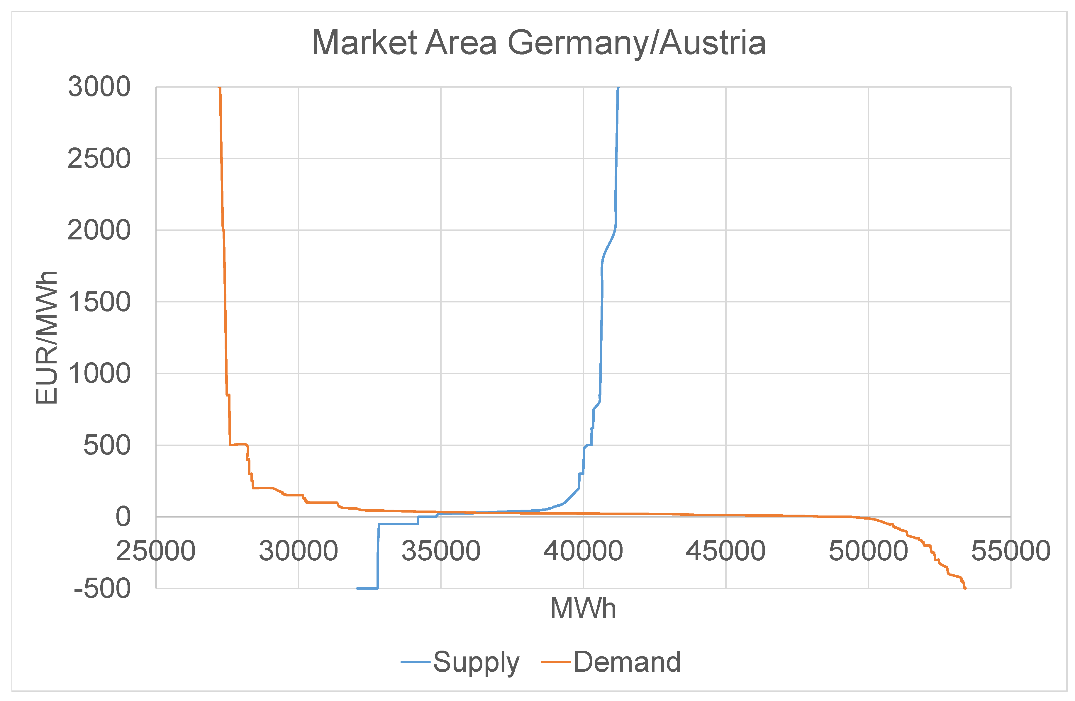
The above introduced regression model has been estimated individually for each hour of the day. We comment in detail on the salient features of three hourly products (results for other hours of the day are available on request), namely hour 4 (3:00 a.m.–4:00 a.m.), hour 13 (12:00 p.m.–1:00 p.m.), and hour 18 (5:00 p.m.–6:00 p.m.) in order to illustrate the main idea of our modeling approach: market fundamentals impact the Swiss electricity prices differently, depending on the steepness of the supply curve and on the demand profile at different trading periods within one day. We estimated the model separately for working versus weekend days, given that the demand slope is steeper during the week (Monday to Thursday) than on the weekend. The inclusion of demand in our formulation encompasses weather and seasonal effects [14]. Results will be interpreted in the context of the particularities of demand and supply curves for electricity in Germany. In Figure 3, we display for exemplification a typical price clearing result of the auctions for the German/Austrian and the Swiss market for a specific hour in 2016. The supply function, which represents the stack of offers for production quantities in ascending order of prices, distinctively increases through concave, flat and convex regions [10].

Often particularly large or small values of the estimated time-varying coefficients correspond to extreme electricity price levels observed historically. For a comparison with the estimation results, the evolution of Swissix prices from January 2010 to August 2016 is displayed in Figure 4.

In the sequel, we show the evolution of the time-varying coefficients that result from the estimation. We give an economic interpretation of their variation, which results from the increasing impact of renewable energies on power prices, an interchange in production sources etc. Note the corresponding fundamental variables are measured in different units and have different magnitudes. Thus, the values of the time-varying coefficients displayed here are not equivalent with the direct contribution of the various fundamentals to the electricity price. The latter is quantified by the so-called “marginal effects”, which we show in the Appendix A.

5.1. Learning Effect

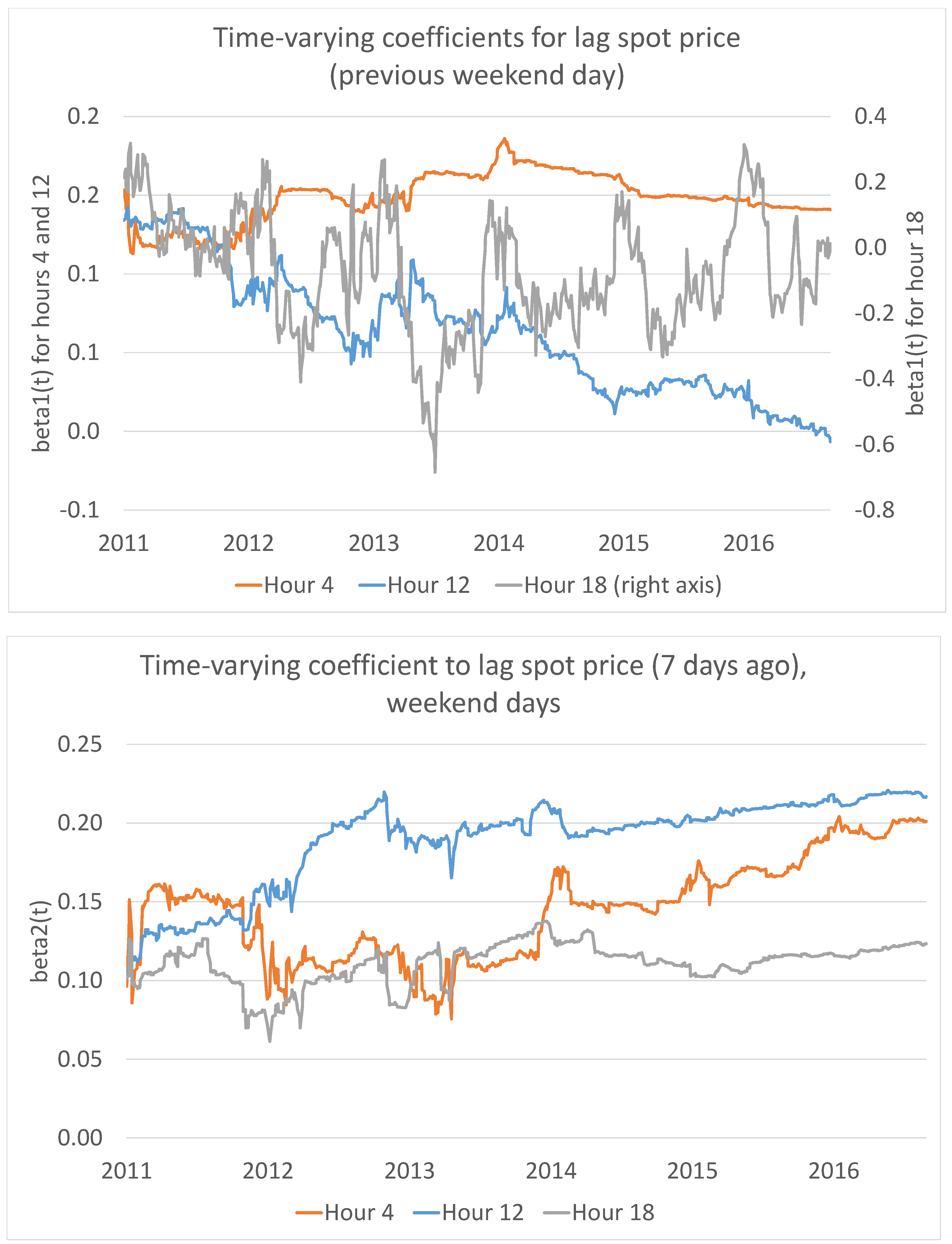
In Figure 5 (upper graph), we observe that the sign of the coefficient of the one-day lagged spot price for hours 12 and 18 is negative most of the time while the coefficient for hour 4 is nearly zero over the entire sample period. The negative sign is intuitive since it reverts the level of electricity prices for a specific hour in the next day, which reflects the typical mean reverting behavior of electricity prices [6]. The coefficients of lagged spot prices reflect the so-called “participant conduct” (see [14] for the UK market and [10] for the market area Germany/Austria).

During the peak hours 12 and 18, there is a high demand for electricity and increasingly scarce supply than for off-peak hours and thus, prices are more volatile. This explains the more pronounced price adaption to one-day lagged prices for these two hours than for hour 4. However, typically electricity prices revert towards their production costs, which explains the negative sign of the coefficients most of the time. Additionally, for hour 18, we observe that coefficients cross the zero axis and become positive, especially in the winter months of each year (evening peaks), when prices are in the upper region of the supply curve and Switzerland imports electricity from Germany. The positive sign of the coefficients in these winter days reflect the clustering effect of extremely large electricity prices (positive price spikes) (Figure 4).

In Figure 5 (lower graph), we observe that there is price adaption of Swissix to its 7-day lagged values as observed in the same hour of the same weekday in the previous week. The spot price lagged by one week corrects the weekly seasonality pattern not fully reflected by the demand curve. In particular, the positive sign of the coefficients indicates that market participants tend to reinforce successful bids previously placed in the market, which is consistent with evidence for the use of market power in electricity price bids found in other studies (e.g., see [14]).

In summary, the upper graph of Figure 5 shows the typical mean reversion pattern in electricity prices for the short-term (one-day lag), but, in addition, there is evidence for the use of market power in the medium-term (one-week lag) as illustrated in the lower graph.

5.2. Influence of Fuel Prices on Swiss Electricity Prices

As discussed in [10], the mid-region of the supply function in the German electricity market, which is characterized by an interchange in production of coal and gas, is flat and price volatility is relatively low. For both generation technologies, coal and gas, producers must hand in emission certificates for every emitted tonne of CO${}_2$. Per unit of generated power, coal requires about twice the number of emission certificates compared to gas. In addition, the operational efficiencies of the various coal and gas plants vary, so that the order of marginal costs tends to be a mix of these technologies: not all coal plants are located below all gas plants in the supply function.

Thus, as commodity prices for coal and gas fluctuate, the sequence of the various gas and coal facilities in this section of the supply function may also interchange. This leads to a competitive and intricate relationship of power prices to gas and coal commodity prices. As a consequence, we expect an adaption process of Swiss electricity prices to prices of fuels used as input in Germany, given that the two markets are interconnected and, furthermore, prices are cointegrated.

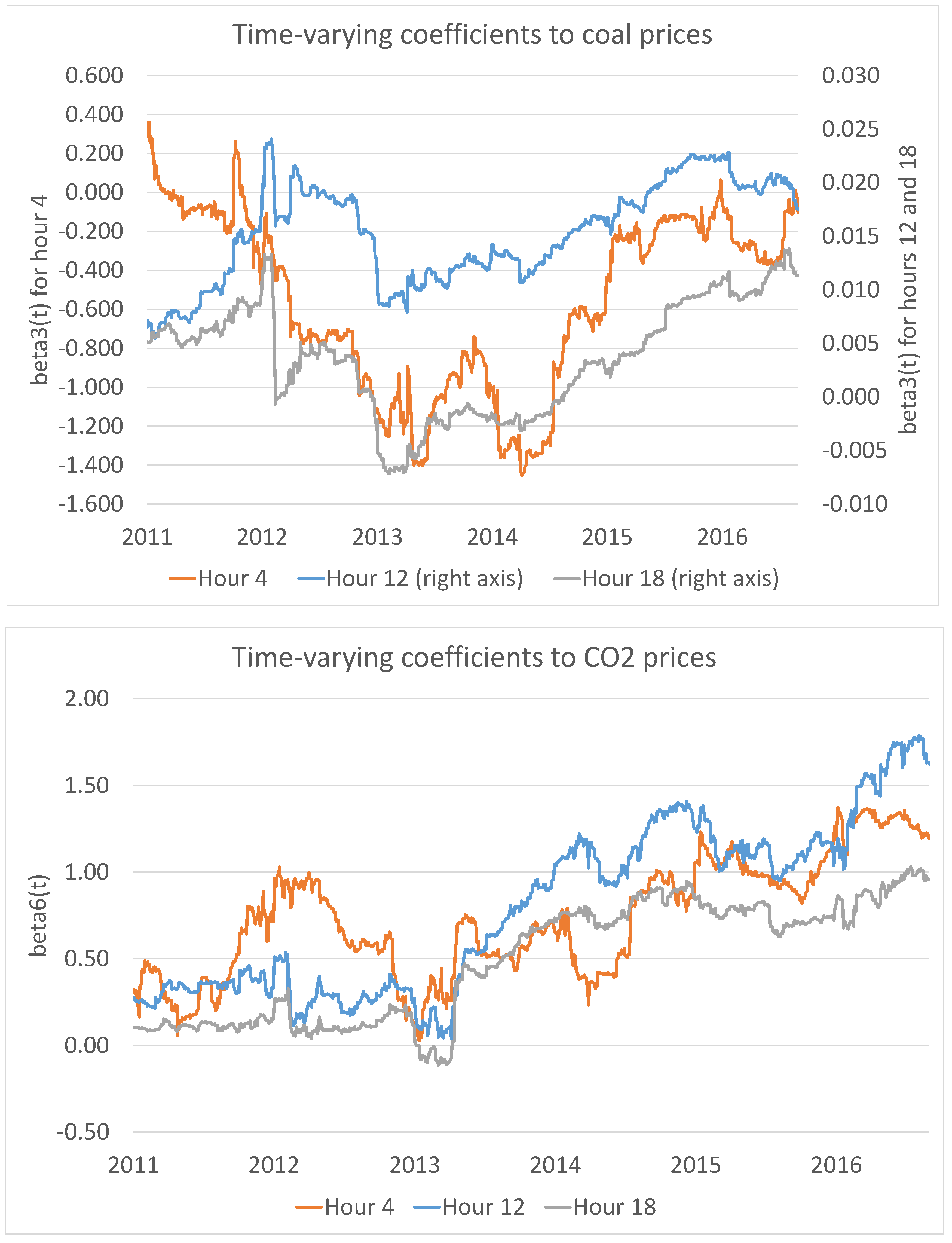
In Figure 6 and Figure 7, we observe that indeed Swiss electricity prices adapt continuously to prices for coal, gas and oil over time. Price adaption to coal and gas occurs, as explained above, due to the interchange between fuels in the mid-region of the supply curve and, furthermore, due to their interaction with renewable energies. An interchange in production between gas and oil, and, from here, implied price adaption to these fuels prices, occurs, for example, in the upper convex region of the supply function, which is characteristic for power markets at times of high demand and increasingly scarce supply. The technologies in this supply region, like gas and oil (diesel), tend to have low capital but high marginal cost (see [10]).

The signs of the coefficients for coal are near zero for the peak hours 12 and 18, but they remain negative over a longer time in the case of hour 4. As discussed above, coal is a cheap production technology (low marginal costs of production), which is situated on the left end of the merit order curve, and electricity production in Germany during off-peak hours (night) is mainly coal based. As Switzerland imports cheap electricity from Germany, there is an adaption to the lower German price level. In consequence, coal prices have therefore a negative marginal effect on Swissix electricity prices.

Switzerland and the EU operate separate emissions trading schemes. In Switzerland, the so-called CO${}_2$ steering taxes (German: Lenkungssteuer) must be paid, which is intended to change the behaviour of consumers and the industry towards a more economic energy usage. However, with respect to the electricity supply side, steering taxes are not a very important price determinant, since Switzerland produces most of its electricity by means of CO${}_2$ neutral technologies like nuclear and hydropower. In addition, for the German market, it has been shown that CO${}_2$ emissions’ certificate prices do not influence producers’ incentives to shift to greener production sources [17]. In Figure 6 (lower graph), we observe that Swissix shows price adaption to the German CO${}_2$ prices with an increasing trend after 2013. This can be explained by an increasing share of fossil-based fuels among the electricity imports from Germany after 2011 (see Table 1), which leads to a pass-through effect of CO${}_2$ prices.

In Figure 7 (upper graph), we observe cross-border positive marginal effects of gas prices on Swissix. The price adaption comes from the interchange between gas/coal in the mid-region or gas/oil in the convex regions of the supply curves. Further adaption comes from the substitution between gas (flexible technologies) and the volatile photovoltaic and wind infeed. High/low wind/PV production moves the supply function to the right (left) and the higher cost gas facilities are pushed out of (into) action. There are no increasing marginal effects from gas over time since gas power plants have been shut down in Germany due to the competition from renewable energies.

We also observe spikes in the evolution of gas coefficients, especially during the winter days, which correspond to electricity price spikes in Figure 4. This shows that Swissix price spikes were due to the more expensive gas-based production imported from the German market. Often, in winter days, the coefficients for hour 18 are higher, due to the so-called “evening peak”, than for hour 12. For hour 4, when prices are in the concave region of the supply curve and gas is typically not used, coefficients for gas are less volatile and induce no price adaption.

For the interpretation of coefficients for oil, we should keep in mind that the percentage of oil in the German electricity production is negligible (see Table 1). This effect is due to the increasingly competitive conditions in the German market, where traditional gas and oil plants have been replaced gradually in production by photovoltaic and wind. Because oil is not burned in the night, we display the coefficients only for the peak hours. We observe little price adaption to oil and furthermore marginal effects close to zero.

5.3. Influence of Demand and Supply

Since electricity is produced to meet demand instantaneously, with yet very little storage options by end-users, hourly variations in price are due to fluctuations in demand that are mapped through the nonlinear supply function to prices, and also through changes in the shape of the supply function itself due to availabilities of wind, solar and other sources of power, as well as the pricing strategies of generators (see the discussion in [10]). In Figure 8, we observe that Swissix prices adapt to shocks in demand and power plant availability (as a measure for electricity supply in Germany). The marginal effects of demand are positive for all hours. A high expected demand in the German market increases power prices there, and this increase will be passed to the prices of neighboring importing countries.

During the night, demand and also the planned capacity are generally low. As a consequence, the system is more sensitive to the fluctuant infeed from wind. Since the inflexible coal facilities have high shut-down and start-up costs, producers are willing to accept prices below their marginal costs in order to generate continuously. Hence, the large (negative) marginal effects of power plant availability (PPA) for hour 4 reflect the deeply discounted and even negative offer prices at the low end of the supply function.

5.4. Influence of Renewable Energies

The infeed from renewable energies has been increasing continuously over the investigated period, as shown in Table 1. Renewables are situated in the lower region of the merit order curve and shift it to the right. Hours with high renewables supply cause difficulties for other generating facilities that might be inflexible and should run continuously (nuclear, district heating and industrial co-generation facilities, as well as some large coal power stations). As outlined above, these inflexible facilities accept negative marginal returns in order to generate continuously which leads to lower electricity prices.

In Figure 9, we show that wind and PV in Germany have a decreasing effect on Swiss prices as well. The continuous price adaption to renewables reflects the substitution in production with traditional fuels as gas or oil in the flat mid-region and upper region of the supply curve (similar results have been found in the analysis of [10] for the German price index): when wind and PV production is high (low), the supply function is moved to the right (left), and gas facilities with higher marginal cost are turned off (on). As expected, there are larger marginal effects of the wind during night hours, due to the inflexibility of coal plants adapting to unexpected extra supply from wind.

This result is of significant relevance for the Swiss policy concerning the local law for renewable production: Switzerland imports lower electricity prices due to the renewables policy in Germany. In particular, due to the high infeed of photovoltaic during peak hours, the spread between Swissix peak and off-peak prices narrowed significantly over time, which results from the market interconnectedness with Germany. The reduced spreads impacted the profitability of pumped-storage hydropower plants severely. Additional incentives for investments in renewable energies or subsidies for hydropower in Switzerland should therefore be considered in the light of this insight.

5.5. Weekend Effect

Figure 10, Figure 11, Figure 12, Figure 13 and Figure 14 replicate the results for weekend days. Overall, we observe that Swiss electricity prices react differently to German market fundamentals for the weekend rather than for working days. In Figure 10 (upper graph), we observe that the coefficients of one-day lagged spot prices (here: previous weekend day in the sample) are positive for hours 4 and 12 but oscillate around zero in the case of hour 18.

On the other hand, there is more price adaption of Swissix to one-day lagged spot prices for hours 12 and 18, when the electricity production is situated in the convex region of the supply function (plants with higher marginal costs run to supplement the residual demand), and prices are more sensitive to changes in demand and, thus, more volatile. This is consistent with our interpretation of the similar graph for working days (Figure 5): at the convex region of the supply function, conduct (one-day lagged spot prices) tends to be a more important feature of price formation than demand, supply or fuel price fundamentals.

There is a descending trend in the marginal effects of one-day lagged spot prices for hour 12. This reflects that prices tend to lose the autoregressive nature since more photovoltaic has been fed into the electricity grid over time and, therefore, has a higher impact on the price formation process. The positive coefficients for hours 4 and 12 suggest the exercise of market power. However, overall, the absolute values of the coefficients are lower for the weekend rather than for working days. However, the exercise of market power becomes more obvious during the weekend rather than working days since, for the latter, coefficients for hour 12 stay positive over time.

Similarly to the working days (see Figure 5), the coefficients of seven-day lagged spot prices remain positive, which confirms our previous results that market participants tend to reinforce previously successful bids (use of market power as shown in the study of [14] for the UK market).

The marginal effects of coal on the Swiss electricity prices on the weekend are negative over almost the entire sample period 2011–2016 for all hours (see Figure 11, upper graph). This shows that, independent of where the intersection point of the demand and supply curves is located in various hours of the day, Swiss electricity prices are marginally reduced by the low price level of coal-based electricity in Germany. The suppressing effect on prices is more obvious for the night hour 4, when the electricity in Germany is mainly produced by coal. This is similar with our insights from the analysis of working days (see Figure 6). In Figure 11 (lower graph), coefficients of CO${}_2$ show no clear trend and have overall a very small magnitude, so the effect of CO${}_2$ on Swiss electricity prices is negligible for the weekend.

In Figure 12 (upper graph) we observe that there are positive coefficients of gas prices and the price adaption is more pronounced for hour 12. A similar picture has been obtained in the case of working days: At noon gas is the marginal unit and, thus, more adaption of electricity to gas prices is observed. As mentioned already before, in the convex region of the merit order gas and oil are typically interchanged in production, and this explains partially the price adaption pattern of coefficients. In addition, adaption occurs when there is photovoltaic infeed which is fed with priority in the electricity grid and replaces temporarily the flexible gas power plants in production. Still, gas power plants are kept on running to balance out demand in days when PV is unavailable. We computed in addition the marginal effects of gas prices on electricity prices expressed in EUR/MWh. As shown in Table 1, there has been a decrease of marginal effects of gas prices on electricity prices after 2013 “compensated” by a continuous increase (in absolute values) of marginal effects from PV. This reflects the shift in the merit order curve.

In Figure 12 (lower graph) we observe that an increase in oil prices causes a decrease in Swissix prices. The intuition is that, as gas and oil are complementarily used in production in the convex region of the merit order and gas plants are flexible, increasing oil prices create incentives to switch to gas as the cheaper technology. This explains the indirect decreasing effect of oil prices on Swissix.

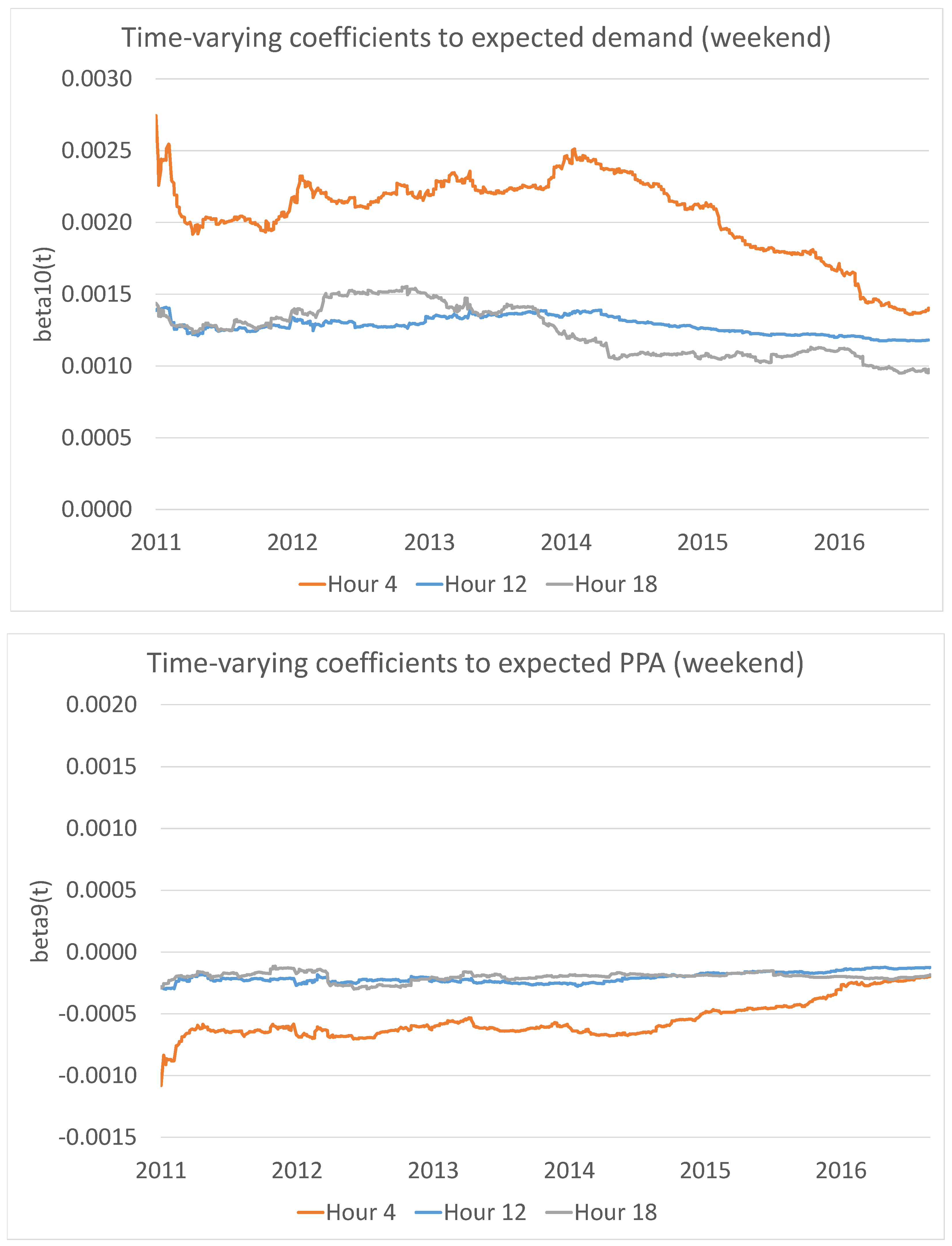
The coefficients of demand for the weekend in Figure 13 resemble the pattern observed during working days (Figure 8). As expected, positive shocks in demand increase prices. The coefficients for power plant availability are also negative for hours 12 and 18. If an excess of capacity meets a low and inelastic demand for electricity, weekend power prices decrease significantly. Due to the low demand on Saturdays and Sundays, this effect is even more pronounced than for working days where negative coefficients of power plant availability occurred only for hour 4.

In Figure 14 we observe that wind and PV have dampening marginal effects on the Swiss electricity prices also during weekend days. The pattern of wind and PV coefficients resemble our results in Figure 9 for working days. Again, the decreasing marginal effect of wind on Swissix is most pronounced during the night, which is consistent with previous results which link high frequency of wind infeed in the night to very low levels of electricity prices (see [6] for the German/Austrian market).

With respect to PV, we observe slightly larger marginal effects (in absolute values) of PV on Swissix on the weekend rather than during working days. This is intuitive since during working days the intersection point of the demand and supply curves is located in the convex region of the merit order and, thus, gas and oil are turned on to supplement the higher demand. When there are higher levels of PV infeed, generation with the latter is reduced accordingly to avoid oversupply, which is reflected in price adaption and substitution effects between market fundamentals. However, on the weekend, the supply is mainly coal based, so any excess of PV infeed will decrease prices more since coal plants are costly to shut down. In other words, high levels of PV infeed reduce prices faster during weekend than during working days, which is reflected in the absolute values of the coefficients.

5.6. Model Significance

In

Table 7. Goodness of fit, for morning, noon and afternoon hourly blocks for working days, including renewable energies wind and PV.

Hourly Blocks	Morning	Noon	Afternoon	Evening	Night
	(Hours 7–10)	(Hours 11–14)	(Hours 15–18)	(Hours 19–24)	(Hours 1–6)
$R^2$	0.491	0.644	0.766	0.785	0.741
Adjusted $R^2$	0.467	0.627	0.754	0.774	0.728
MAE (EUR/MWh)	4.224	4.089	4.163	3.865	3.999
DW	2.354	2.349	2.330	2.238	1.946
LLF	−4086.534	−4050.761	−4051.969	−3931.799	−4060.185

and

Table 8. Goodness of fit, for morning, noon and afternoon hourly blocks for weekend days, including renewable energies wind and PV.

Hourly Blocks	Morning	Noon	Afternoon	Evening	Night
	(Hours 7–10)	(Hours 11–14)	(Hours 15–18)	(Hours 19–24)	(Hours 1–6)
$R^2$	0.736	0.806	0.813	0.822	0.714
Adjusted $R^2$	0.710	0.787	0.794	0.804	0.685
MAE (EUR/MWh)	5.457	5.288	5.321	4.067	4.877
DW	2.178	1.948	1.932	2.100	2.119
LLF	−2124.511	−2112.721	−2110.272	−1949.686	−2062.411

, we assess the goodness of fit for our model by computing the $R^2$, mean average error (MAE) and Durbin–Watson (DW) statistics. Log-likelihood function (LLF) values of the model estimates are shown in the last rows of the tables. During working days, the variation of Swissix prices explained by the the time-varying fundamental model is 49% for morning hours and increases to almost 80% for the evening. Note that the $R^2$ values for working and weekend days cannot be compared directly since, in the latter case, there are significantly less observations available for the estimation. Indeed, the mean average error (MAE) expressed in EUR/MWh shows larger deviations for the weekend than for working days. Furthermore, we conclude that model residuals show no (or very little) serial correlation, as indicated by the Durbin–Watson (DW) test statistics.

In addition to the results discussed above, we estimated also a version of the time-varying regression model where wind and PV were excluded. This should help assess to what extent infeed from renewable energies in Germany explains the variation of electricity prices in Switzerland and how relevant they are for the Swissix price formation process. Results in

Table 9. Goodness of fit, for morning, noon and afternoon hourly blocks working days, excluding renewable energies wind and PV.

Hourly Blocks	Morning	Noon	Afternoon	Evening	Night
	(Hours 7–10)	(Hours 11–14)	(Hours 15–18)	(Hours 19–24)	(Hours 1–6)
$R^2$	0.469	0.625	0.763	0.764	0.657
Adjusted $R^2$	0.445	0.608	0.752	0.753	0.641
MAE (EUR/MWh)	4.646	4.346	4.392	4.260	4.676
DW	2.296	2.246	2.227	2.190	1.839
LLF	−4223.906	−4154.082	−4154.176	−4106.158	−4285.626

and

Table 10. Goodness of fit, for morning, noon and afternoon hourly blocks weekend, excluding renewable energies wind and PV.

Hourly Blocks	Morning	Noon	Afternoon	Evening	Night
	(Hours 7–10)	(Hours 11–14)	(Hours 15–18)	(Hours 19–24)	(Hours 1–6)
$R^2$	0.677	0.747	0.756	0.785	0.627
Adjusted $R^2$	0.645	0.722	0.733	0.764	0.590
MAE (EUR/MWh)	6.300	6.239	6.139	4.527	5.639
DW	1.957	1.912	1.851	2.048	2.110
LLF	−2231.725	−2220.441	−2227.014	−2027.281	−2152.368

show that by excluding both wind and PV from the model, the explained variation drops particularly for the weekend when demand is low and the share of renewable energies in the overall production is relatively high, compared to working days. In all cases, the MAE increases by roughly 10% when wind and PV are not taken into account. This illustrates again that the infeed of renewable energies in Germany clearly has an impact on electricity prices in Switzerland.

6. Conclusions

6.1. Goal of the Paper

The goal of this paper is to identify marginal effects of fuel prices and renewable energies that impact cross-border Swiss electricity prices given the interconnector between Switzerland and Germany. We extended the analytic framework proposed in [6] that referred solely to the German market. These insights are important to energy policy makers given that Switzerland debates currently on the need to invest in renewable energies and flexible storage devices. In this context, an overview of cross-border effects from renewables and other production sources in the neighboring countries on Swiss electricity prices are of great relevance. We found that market fundamentals that traditionally impacted electricity prices in Germany show cross-border effects on the neighboring Swiss market. In addition to the original study, we disentangled the effect of fundamentals on prices not only between different hours of one day, but also between working versus weekend days.

6.2. Main Findings

We found that Swiss and German electricity markets are cointegrated and cross-border effects are statistically significant. Furthermore, it could be observed that Swissix prices adapt continuously to fuel prices, renewable energies (wind and photovoltaic), participant conduct and demand–supply curves that are specific for the German market. Results lead to an intuitive economic interpretation, where marginal effects of fundamentals depend on the different locations of the intersection point between demand and supply curves within a day. Hence, fundamentals impact Swissix prices differently, dependent on the time of the day, given that the input mix differs across peak and off-peak delivery periods.

Results show furthermore that during working days fuel prices of coal, gas and (to some extent) oil have time-varying marginal effects on Swiss electricity prices and their coefficients are comparatively large in absolute values. Depending on the time of the day where prices are observed, price adaption to fuels can be explained by the substitution among those, in particular coal and gas in the mid-region of the supply curve, or by their interaction with renewable energies such as gas/wind or gas/PV when prices are in the upper (steeper) segment of the merit order curve. However, the impact of fuel prices drops during weekends when demand is lower and, thus, the price formation arises mainly from the interaction between coal and renewable energies.

6.3. Importance to Policy Makers

In summary, Switzerland imports cheaper electricity prices over time, marginally due to the increase in renewable energies in its neighbour country Germany. Indeed, we found time-varying negative marginal effects of wind and PV on Swiss electricity prices, independent from the time of the day and for all weekdays. This result is of great relevance for Swiss policy makers with respect to the local regulation of the promotion of renewable energies: Switzerland imports lower electricity prices due to energy transition in Germany. In particular, because of the high infeed of PV during peak hours the spread between Swissix peak and off-peak prices narrowed significantly over time, as a consequence of market interconnectedness with Germany. Incentives for investments in renewable energies in Switzerland as well as subsidies for hydropower should be considered in the light of these insights. Overall, the understanding of the risk drivers of electricity prices is of great importance for risk management, production planning, as well as for policy makers for the derivation of long-term energy scenarios.

6.4. Further Research

This study looks only at cross-border effects given the electricity exchange between Switzerland and Germany. A broader analysis of these effects for the existing interconnectors to other countries is the subject of further research. In addition, it is important to disentangle marginal effects for different price regions, not only for different hours within one day.