Decision Support Tool for Offshore Wind Farm Vessel Routing under Uncertainty

1
Department of Electronic & Electrical Engineering, University of Strathclyde, Glasgow G1 1XW, UK
2
Department of Management Science, University of Strathclyde, Glasgow G1 1XW, UK
*
Author to whom correspondence should be addressed.
Energies 2018, 11(9), 2190; https://doi.org/10.3390/en11092190
Submission received: 30 July 2018
/
Revised: 16 August 2018
/
Accepted: 19 August 2018
/
Published: 21 August 2018
Abstract
:This paper for the first time captures the impact of uncertain maintenance action times on vessel routing for realistic offshore wind farm problems. A novel methodology is presented to incorporate uncertainties, e.g., on the expected maintenance duration, into the decision-making process. Users specify the extent to which these unknown elements impact the suggested vessel routing strategy. If uncertainties are present, the tool outputs multiple vessel routing policies with varying likelihoods of success. To demonstrate the tool’s capabilities, two case studies were presented. Firstly, simulations based on synthetic data illustrate that in a scenario with uncertainties, the cost-optimal solution is not necessarily the best choice for operators. Including uncertainties when calculating the vessel routing policy led to a 14% increase in the number of wind turbines maintained at the end of the day. Secondly, the tool was applied to a real-life scenario based on an offshore wind farm in collaboration with a United Kingdom (UK) operator. The results showed that the assignment of vessels to turbines generated by the tool matched the policy chosen by wind farm operators. By producing a range of policies for consideration, this tool provided operators with a structured and transparent method to assess trade-offs and justify decisions.
1. Introduction
At the end of 2016, there was 12.6 GW of grid-connected offshore wind capacity in Europe; this number is projected to increase to 25.6 GW by 2020 [1]. Reducing the cost of energy to ensure competitiveness with other electricity sources will be one of the key challenges that the industry will face in the near future [2]. The yearly cost of post-warranty operations and maintenance (O&M) activities for a 4-MW offshore wind turbine is around £648,000 [2]. In the future, the number of offshore wind turbine visits may increase due to the untested reliability record of large direct drive machines, increased complexity of electrical components, and higher failure rates in late life. Simultaneously, with farms being located further offshore, the complexity of planning the use of vessels to carry out O&M increases. The improvement of strategies through the use of decision-making tools is a priority for offshore wind O&M [3].
Currently, there are eight offshore wind farms in Europe with over 100 turbines (European wind farms with 100+ turbines: London Array, Gemini, Gwynt y Môr, Greater Gabbard, Anholt, Rampion, West of Duddon Sands and Walney); each year there will be days on which more than 20 turbines require either a preventative or corrective maintenance action. The development of a vessel routing strategy, i.e., the assignment of turbines to vessels and the order in which maintenance actions are carried out, is a short-term decision-making problem. Operators are under considerable pressure as the time to make these decisions is often constrained; in many cases, the plan is created either on the day or the night before. Computing all of the possible vessel routing policies for problems with over 20 turbines exceeds the capability of a modern computer, not to mention a human being. The problem is computationally challenging due to its size, but also due to multiple constraints related to the number of technicians available, vessel carrying capacity, and the time in which the policies have to be completed. Furthermore, planning vessel routing for offshore wind farms is made more difficult by numerous uncertainties. Taking human error, weather, incorrect fault diagnosis, or estimated maintenance action time into account when developing a vessel routing strategy is challenging.
Irawan et al. [4] provided a literature review of solution methods of routing problems in the context of offshore wind turbine maintenance. They propose a solution based on the Dantzig–Wolfe decomposition method combined with a mixed-integer linear program (MILP). This approach, although computationally effective, lacks the flexibility to incorporate the possibility of repairs taking longer than expected. Furthermore, in the last five years, the problem of vessel routing for offshore wind farms was tackled by Dai et al. [5], who used a branch and bound method, Zhang [6], who used Ant Colony Optimisation, and Stålhane et al. [7], who used a path-flow model. To date, no model for vessel routing optimisation in the offshore wind domain attempted to take into account uncertainties on the expected maintenance action time and wave height, which are a consideration when planning vessel routing in real life. While vessel routing has also been a subject of research in other fields, e.g., the oil and gas industry and container ship logistics, these problems are characterised by significantly different constraints. In the authors’ opinion, the solutions to these problems are no more applicable to the problem at hand than standard vehicle routing problems (VRP), which were reviewed exhaustively by Caceres-Cruz et al. [8]. A review of relevant VRP models that are capable of dealing with uncertain inputs is provided in Section 2.2.
The problem at hand is a variation of a Capacitated Vehicle Routing Problem with Pickup and Delivery (CVRPPD) with route duration constraint. However, there are numerous differences in the assumptions and constraints between the standard CVRPPD and the real-life problem of planning offshore O&M actions. In the latter problem, time windows for pick-up have hard bounds that are never exceeded as well as soft bounds. Technicians need to be picked up by the vessel that dropped them off. Each route starts and ends at the same maintenance base. In the real-life problem, crew transfer time (vessel to turbine) and variable vessel speed need to be modelled. While the main objective of many standard solutions to a VRP is to minimise the distance travelled, this is not a key factor when deciding vessel routing for offshore wind farms; turbine availability, for example, is a much more important parameter. Finally, operators are sometimes faced with a severe lack of resources, making it impossible to visit all of the turbines requiring maintenance, meaning that they have to prioritise the turbines to be serviced on the day. Resource shortages may result in a backlog of maintenance activities leading to long wind turbine downtimes [9]. The real-world problem features numerous constraints and uncertainties; the number of possible routing plans is high, and the time that operators have to solve the problem is limited. Hence, it would seem that the best approach to solving this problem would be to use a mathematical model. However, according to the interviews the authors have conducted with United Kingdom (UK) offshore wind farm operators, vessel routing plans are still made by the operators, without the use of decision support tools. A variety of methodologies that could aid real-life decision making were proposed by the research community, but there is no evidence of any practical application of those proposed solutions. The authors believe that this is partly due to the academic models being unable to consider all of the relevant constraints and produce user-friendly outputs that could be easily interpreted by the operators. The approach proposed in this paper attempts to address these issues, bridging the gap between the industry and research domain.
This paper expands on the work done in the authors’ previous publication [10]. While the solution of the inner problem remains the same—it is based on case-dependent decision flowcharts—the exhaustive search used to solve the master problem has been replaced by formulating the problem as a mixed-integer programming problem and solving it using an IBM CPLEX Optimizer (12.71, IBM, Armonk, NY, USA). Secondly, calculation of the probability of successfully carrying out all of the repairs within a policy was implemented. The user is now able to specify their risk aversion, depending on the circumstances. For example, policies visiting fewer turbines but with a higher success probability can be favoured in highly uncertain weather conditions.
The proposed decision support tool is capable of automatically generating a range of candidate policies in short computational time. Providing wind farm operators with multiple strategies, which can be discussed and evaluated, can encourage improved decision making. Since real-world expected task durations typically have a large variance, the inclusion of uncertain maintenance action times significantly improves the quality of results compared to models based on deterministic task durations.
This paper is organised as follows: Section 2.1 describes the model’s structure, and Section 2.2 outlines the methodology for incorporating probability into the decision-making process. Section 3 presents synthetic data and real-life case studies, respectively. Finally, the conclusions of the paper are summarised in Section 4.
2. Materials and Methods
2.1. Model Structure
As pointed out by Irawan et al. [4], decomposing a VRP into outer problem (sometimes called a master problem) and inner problem is a common denominator in recent advances in capacitated VRP solution methods. The former is a problem of assignment of turbines to vessels, while the latter is a problem of ordering turbine visits. A similar approach was used in the model described here; an overview of the split between the inner and outer problems is shown in Figure 1.
The solving procedure begins by enumerating all of the possible clusters of turbines. The maximum number of turbines in a cluster (η) was limited to four. It was shown by Irawan et al. [4] that setting η to four yields, in most cases, answers within 97% of the optimal solutions. Limiting η decreases the computational time significantly. In practice, the number of turbines that a single vessel can maintain on one day will be limited by its capacity and the time available.
Next, clusters of turbines are each assigned a vessel. As the model considers non-homogenous vessels, it is possible that repairs in certain clusters may only be possible to complete within the time constraint by the vessels with a higher cruise speed. Therefore, each cluster of turbines is matched with each of the vessels.
Ordering decision flowcharts, which were verified by an offshore wind farm operator, were used to solve the inner problem (flowcharts, along with a detailed description of the inner problem solution procedure, are included in the Supplementary Material). At the inner problem stage, any clusters that do not match user-specified constraints, such as an available time window or vessel capacity, are eliminated. The value of all of the remaining clusters is calculated as discussed in Section 3.
The outer problem was formulated as a mixed-integer programming problem, with the objective function as shown in Equation (1) and the following constraints:
- Each turbine is visited by one vessel only (Equation (2)).
- Each cluster can only be assigned one of the vessels (Equation (3)).
- The number of technicians required does not exceed the number of technicians available on the day (Equation (4)).
Note that other constraints, such as vessel capacity, are dealt with at the inner level problem.
where K is the set of feasible routes, i and j are the individual turbine and vessel identifiers, respectively, Fpk is the value of cluster k (Equation (8)), Qk is a binary decision variable (1 if route k is selected, 0 if not), Sik is a binary parameter (1 if turbine i is on route k, 0 otherwise), Vkj is a binary parameter (1 if vessel j is on route k, 0 otherwise), Dk is the amount of technicians required to carry out maintenance actions on route k, and E is the number of technicians available on the day.
The outer problem was solved using IBM CPLEX Optimizer software [11]. It uses a branch-and-cut method to maximise the overall value of the policy by choosing a set of individual clusters that satisfy all of the constraints. The following section describes the methodology used to incorporate uncertainties into the value function.
2.2. Calculating the Probability of Carrying out Successful Maintenance Actions
There are multiple uncertainties that need to be taken into account when planning offshore wind farm operations. There is an uncertainty regarding the expected maintenance action time, which may vary depending on the type of maintenance action. On days with high waves, it is uncertain whether technicians will be able to transfer from the vessel onto the turbine. Modelling such uncertainties can be challenging, but it is important to consider them, as these real-life uncertainties do affect the day-to-day decision making.
One of the approaches for dealing with uncertainty when solving VRPs is robust optimisation. It allows specifying the uncertainty bounds on parameters. The solution produced is resilient to changes in inputs. Examples of recent applications of robust optimisation in VRPs include Sun and Wang [12], who proposed a solution to a VRP with uncertain transportation costs and customer demands, while Allahviranloo et al. [13] applied parallel genetic algorithms to a VRP with limited resources, under uncertainty.
Particle swarm optimisation has been used by Moghaddam et al. [14] and Marinakis et al. [15] in cases with uncertain demand. However, the nature of uncertainty in the problem of offshore wind farm maintenance optimisation is different: a potentially large uncertainty is associated with the duration of repair. A single maintenance action taking longer than expected may cause a snowball effect, leading to failed repairs on multiple turbines due to lack of time.
An alternative approach to solving this problem is to formulate it using soft time windows, in which arrival outside of the specified time window is penalised. Examples of such models include Tas et al. [16] and Russell and Urban [17], who both used tabu search to solve problems with uncertain travel time and soft time windows.
A comprehensive review of stochastic VRPs was conducted by Oyola et al. [18]. It covers a variety of approaches that are used to solve logistic problems under uncertainty, including a number of papers in which the servicing time is uncertain. These include Li et al. [19], Lei et al. [20], and Chen et al. [21] who all assumed normal distribution service time. The aforementioned papers by Tas et al. [16] and Russell and Urban [17] use gamma and Erlang distributions for travel times, respectively, while Gomez [22] modelled variable travel times using a wide range of distributions, which included Erlang, Burr, and lognormal distributions. Problems with uncertain service times have also been tackled by Bertsimas & Ryzin [23] and Chepuri & De-Mello [24], who used constrained optimisation and the cross-entropy method, respectively.
2.2.1. Methodology
An approach is proposed in which uncertainties are modelled by calculating the probability of maintaining all of the turbines within a cluster. We assume that the time available to carry out all of the maintenance actions on the day (i.e., time window) is a hard constraint, meaning that the recourse action is to return to base before the deadline, even if it means leaving maintenance actions unfinished.
Prior to running the optimisation tool, the decision maker specifies Ptij, Pdi, and Pri. Ptij is the probability of successfully transferring the crew onto turbine i using vessel j, depending on the sea state and vessel capabilities. Pdi is the probability that turbine i was correctly diagnosed, and Pri is the probability that maintaining turbine i takes less time, or is equal to the time available for that maintenance action. Assuming that G is the set of turbines assigned to vessel j, the probability that vessel j will be able to carry out all of the scheduled maintenance on a particular day is defined as:
Specifying the forecasted wave height at each turbine allows modelling a wave field that varies across the wind farm. Through this approach, more capable vessels can be encouraged to visit turbines that are expected to experience higher waves.
The probability of a fault on a turbine being correctly diagnosed was introduced, as the operator may not always be certain what maintenance action is required given the alarm code received. If that is the case, a low Pdi is specified. In practice, values of user-defined probabilities, e.g., Pdi, can be obtained by systematically logging every event of incorrect diagnosis and alarm code associated with it. From this, the likelihood of being able to successfully repair an issue given the type of alarm can be calculated. Similar procedures can be implemented for other uncertainties.
Finally, the probability of the vessel exceeding the time window, due to individual maintenance actions on given turbines taking longer than expected, is taken into account using Pri. Calculating the maximum time available for each maintenance action depends on three factors: the slack time in the policy, the order in which actions are carried out, and the probability distribution function (PDF) of expected maintenance durations. While the user can specify any PDF, gamma distribution with a long tail (positive skewness) was used in this work, as it mimics the real world maintenance action times. Gamma distributions can be added easily (provided that they have the same scale parameter).
The time available for maintenance at a given turbine is calculated by adding the expected duration of repair and slack in the policy. The time difference between the vessel’s estimated arrival back at base and the end of the time window is the critical path slack (Y), which is divided among all of the maintenance actions on the day. Non-critical path slack (Z) can also occur in some policies, for example, if a vessel is idly waiting for the last of the crews to finish repairs, having previously collected other crews. The non-critical path slack is also divided among the relevant maintenance actions. If Ri is the expected maintenance duration on turbine i (mean of user-defined gamma distribution), the time available for repairs on turbine i (Xi) is calculated using the formula shown in Equation (6).
Once Xi is calculated, the probability of meeting the time constraint is obtained from the cumulative distribution function chosen by the user. The calculation of Pri for gamma distribution is shown in Equation (7):
where a and b are the shape and scale parameters of gamma distribution. Note that the mean value of the distribution is the same as the expected maintenance action time.
2.2.2. Risk Aversion Factor and Value Function
Risk aversion factor (A) is a user input, which translates the Pvj (Equation (5)) of all of the policies into value added to the rewards for maintaining turbines. The overall value of policy p (Fp) is defined in Equation (8), where Cri is the cost of maintaining wind turbine i, Cfj is the cost of fuel incurred by vessel j, Cvj is the hire cost of vessel j, and Umean is the average reward across all of the turbines. Ntj is the number of turbines visited by vessel j, and was included in Equation (8) to normalise the added reward into per-turbine value. This prevents the outer problem solution algorithm favouring policies with few turbines and high Pvj.
The user may choose to set the reward of all of the maintenance actions to an arbitrary number, if all of the turbines have the same priority. Alternatively, the relative value of maintaining all of the turbines depending on the type of action required and external factors such as weather can be calculated as shown in Dawid, McMillan & Revie [25].
If A is set to 0, the calculation of probability will not affect the choice of policy. The larger the A, the more influence probability calculation will have on the policy chosen by the model. The user may wish to specify a high risk-aversion factor on days when the weather forecast is highly uncertain. A high risk-aversion factor favours policies in which:
- (a)
- There is an ample amount of slack time to allow for some repairs taking longer than expected. If high risk aversion is specified, the model is encouraged to select faster vessels to carry out repairs on clusters that are expected to take longer.
- (b)
- Assignment of vessels with inferior transfer capability to turbines with expected high waves is discouraged.
- (c)
- Turbines that have a high likelihood of being maintained (low or no possibility of incorrect diagnosis) are prioritised.
The introduction of a non-zero risk aversion factor favours policies with either higher cost, or lower rewards for turbine repairs compared to the optimal solution. Some of the reasons why the user may wish to specify a non-zero risk aversion factor despite it encouraging lower value policies are as follows:
- (a)
- Planning to visit fewer turbines does not mean that fewer turbines will be maintained; the opposite may be true in the presence of uncertainties on the expected maintenance duration.
- (b)
- Leaving unfinished maintenance on the turbine (particularly in the nacelle) often results in wasted technician time. For example, if the last maintenance action of the day takes longer than expected, technicians may need to leave the turbine and head back to base without completing the task to comply with maximum working hours regulations. Time is then wasted the next time the turbine is visited, e.g., the following day, as technicians need to transfer to/from a vessel, and climb up/down the nacelle for the second time.
- (c)
- The assignment of vessels to clusters is no longer based only on its capacity, fuel consumption, and the ability to meet the time constraint, but also on its capability to transfer crews onto turbines in a given wave height.
The benefit of placing a value on the probability of successfully maintaining all of the turbines in a policy is shown in a case study, as described in Section 3.1.
2.3. Evaluation of Policy against Key Performance Indicators (KPIs)
So far, a methodology for generating an optimal policy and incorporating uncertainty into the decision-making process has been proposed. This section describes the procedure used to evaluate the effectiveness of solutions of uncertain scenarios.
The value function presented in Equation (8) attempts to achieve the following KPIs:
- (a)
- Maximisation of the number wind turbine visits.
- (b)
- Maximisation of the number of high reward wind turbine visits.
- (c)
- Minimisation of costs.
- (d)
- Minimisation of the number of unsuccessful repairs (due to uncertainty realisations).
The policies generated by the tool will be evaluated against these KPIs. A random number generator (RNG) combined with a Monte Carlo analysis was used to calculate the average number of turbines that would have been successfully maintained over a high number of iterations if a certain policy was carried out, given the user-specified uncertainties.
In each iteration of the Monte Carlo simulation, three random numbers are generated for each turbine:
- (a)
- One to determine the actual maintenance action time, which is calculated using the inverse of the gamma cumulative distribution function (i.e., inverse of Equation (7)).
- (b)
- One to determine whether the transfer of crew onto the turbine will be possible.
- (c)
- One to determine whether the turbine was correctly diagnosed.
Taking (c) as an example, if the random number that was generated is lower than the probability of correct diagnosis for a given repair type, maintenance can be successfully completed (provided conditions on allowed maintenance time and crew transfer are also satisfied). Determining how many turbines are not fixed due to excessive maintenance action time is more complex. Once actual maintenance durations are generated for all of the turbines using a random number and user-specified cumulative distribution function, a new pick-up order needs to be determined. This is done using the algorithm that determines the pick-up and drop-off order in the sub-problem (see Section 2.1). The new time taken by the policy is calculated and compared against the time window. If the time window is exceeded, at least one of the turbines will not be successfully maintained. The number of turbines actually maintained is calculated by working backwards and calculating which is the first maintenance action not cut short by the need to go back to the O&M base to meet the time constraint.
The number of turbines that were not maintained for all of the aforementioned reasons is added up and subtracted from the total number of turbines that were to be serviced in a given policy. This allows a comparison of the effectiveness of different policies in terms of the average number of turbines that would be visited once uncertainties are realised.
3. Results
This section is divided into two subsections. Case Study 1 (Section 3.1) focuses on a fictional scenario to illustrate the full capabilities of the model. In Case Study 2 (Section 3.2), the tool was applied to a real world scenario.
3.1. Case Study 1
3.1.1. Model Inputs
A fictional wind farm was created to illustrate the capabilities of the model. Turbines were arranged on a 10 × 10 square grid, with 1.1-km separation. The maintenance base was located 80 km from the centre of the wind farm, in the northeastern direction. On a particular day, 20 randomly selected turbines required a maintenance action. The properties of each type of failure, including cost to repair, estimated maintenance action time, number of technicians required, and the weight of spares/tools can be found in Table S1 in the Supplementary Material. The cost of repairs and annual service were adapted from Dinwoodie et al. [26]. Turbine locations and types of maintenance action required on each turbine are shown in Figure 2. Distances between individual turbines and the O&M base are specified in the Supplementary Material.
The rewards for maintaining a turbine depend on the type of repair. Rewards for performing manual reset, minor and medium repair were £100,000. To reflect the importance of high-priority repairs, the reward was set at 120% of the standard repairs (£120,000). Preventative maintenance actions, such as topping up grease and annual service, were associated with a reward of £80,000.
Each value of expected maintenance action duration was associated with a gamma distribution function (as discussed in Section 2.2.1). The shape and scale parameters for each maintenance action are shown in Table S2 in the Supplementary Material. In practise, a realistic gamma distribution could be obtained by logging real-world maintenance durations and fitting a distribution with appropriate parameters to the dataset.
The operators had five vessels available to them: three standard crew transfer vessels (CTVs) and two more capable and faster vessels. It was assumed that three of the vessels were chartered on a long-term basis, meaning that there was no on-the-day charge associated with using them. Hire costs for the remaining two vessels, along with other vessel properties, are shown in Table S3 in the Supplementary Material.
A non-uniform wave field was assumed: turbines 1–20, and all of the turbines that have ID ends with the digits 9 or 0, would experience a wave height of 1.5 m. Standard CTVs may not always be able to transfer crews onto turbines in such conditions. The wave height at all remaining turbines was assumed to be 1.3 m. Values for the probabilities of a successful transfer given the wave height and vessel type can be found in Table S4 in the Supplementary Material. In general, the combination of the aforementioned probabilities and wave height values can be used as a proxy for the expected difficulty of crew transfer, which in reality depends on both wave height and direction.
The total time window for carrying out maintenance actions on the day was 11 h, and the number of technicians available was 45. Crew transfer between vessel and turbine was assumed to take 20 min. Vessel speed when sailing turbine-to-turbine was set at two-thirds of the cruise speed to account for turning and acceleration/deceleration. Due to the limitation of the algorithm used to solve the inner problem (described in more detail in the Supplementary Material and in Dawid et al. [10]), the maximum number of turbines per vessel was limited to four.
3.1.2. Model Outputs
In total, five simulations were run, with the only difference between them being the value of the risk aversion factor, ranging from 0 to 10, as shown in Table 1. All of the simulations were run using MATLAB with embedded IBM CPLEX Optimizer on a 3.4 GHz i7-3770 CPU with 8 GB of RAM and a 64-bit Windows 7 operating system. The total computational time to solve all five cases, including the Monte Carlo analysis, was 215 s.
Not all 20 turbines could be serviced on that day due to a shortage of technicians and vessels. In all five cases, five vessels were used despite specifying hire costs for two of the vessels. The rewards for maintaining additional turbines enabled by these vessels outweighed their hire costs.
As shown in Table 1, increasing A resulted in a decrease of the number of turbines to be visited by technicians. This is closely linked to the drop in expected policy value; as fewer turbines are expected to be maintained, the rewards are reduced.
The performance of policies generated in each of the cases, in terms of the KPIs discussed in Section 3.2, is shown in Table 1. As the risk aversion factor increases, the number of turbines that would have been successfully repaired if those policies were carried out is higher, or the same, as the base case (Case 1). The policies selected in cases 3–5 were more successful than the base case as the impact of uncertainties is taken into account. All five policies planned visits to all four high priority turbines, as the reward for this type of maintenance action was 20% higher.
In Case 1, on average, only 10.8 turbines would have been successfully maintained, despite planning to visit 19 turbines. This number stands at 11.5 for Case 5, which aimed to maintain only 14 turbines. However, this does not necessarily mean that the policy created in Case 5 would be favoured by the operator. The number of man-hours worked on all of the turbines would have been less compared to Case 1, as in Case 5, no medium repairs, which take the longest to complete, were carried out. Furthermore, the policy generated in Case 5 did not make full use of the technicians available to the wind farm operator on this day. The bottom three rows of Table 1 show a breakdown of the reasons why turbines were not successfully maintained in each case. Maintenance actions taking longer than expected were the main cause of unsuccessful visits. As the risk aversion factor increases, the choice of policy is increasingly driven by maximising the overall slack time for each vessel rather than maximising the rewards for repaired turbines. This reduces the difference between the number of turbines planned to be maintained and the turbines actually maintained at the end of the day.
A significant decrease in the number of unsuccessful visits due to unsuccessful transfer can be seen as the risk aversion factor increases. Ten turbines requiring maintenance were located in an area affected by higher significant waves. In Case 1, 3/9 were visited by the more capable vessels, compared to 6/7 for Case 5, which translated to an average reduction of failed vessel-to-turbine transfers of one turbine.
Out of the five cases, the policy in Case 1 had the highest expected value (which does not include the added value due to a non-zero risk aversion factor). Monte Carlo simulation showed that by applying a policy generated in Case 3, which had a significantly lower expected value, on average, it is possible to successfully service more turbines. The increase in successful maintenance actions due to the inclusion of a non-zero risk aversion factor amounted to 14%. This increase came despite the plan for the policy in Case 3 being to visit two fewer turbines compared to the base case. The vessel dispatch plans for the policies generated in cases 1 and 3 are shown in Figure 3 and Figure 4, respectively. Dispatch plans for all of the other cases are included in the Supplementary Material.
Adopting a risk aversion factor of five would, on average, result in the highest number of successfully serviced turbines on the day. On the other hand, ignoring the probability calculation by choosing an A value equal to zero yielded the lowest number of turbines maintained. However, there is no universal, optimal value of A; it depends on the circumstances, such as the number and severity of maintenance actions to be carried out, available resources, and the cumulative probability density function of the expected maintenance action times.
The policy generated in Case 1 (shown in Figure 3) suggested not visiting the turbine requiring an annual service (i.e., non-critical maintenance action). The policies in cases 2–5 all featured medium repairs not being completed. Medium repair had a degree of uncertainty associated with it, meaning that there was a 10% chance that the crew would not be able to bring the turbine back online, despite spending the required amount of time trying to repair it. A non-zero risk aversion factor and higher cost of repair discourages the selection of medium repairs in cases 2–5.
The recommended pick-up and drop-off order for each vessel and the probability of successfully completing all of the maintenance actions by each vessel are shown in Table 2. The order of visits for all of the remaining cases can be found in Table S5 in the Supplementary Material. The pick-up order was determined based on the expected maintenance action times; it can change depending on the actual maintenance action duration.
As indicated in Table 2, vessels 3–5 in Case 1 were assigned to visit four turbines while carrying three teams of technicians. Each of those vessels carried one crew visiting two different turbines in one day. While this does ensure an efficient use of resources, it also decreases the probability of finishing all of the maintenance on time. In contrast, all of the teams of technicians in Case 3 only visited one turbine. As a result, the probability of repairing all of the turbines was higher, but the number of turbines to be visited was lower.
It should be noted that in Case 3, the probability of successfully maintaining all of the turbines by vessels 4 and 5 was significantly lower than vessel 3, which was due to it visiting one fewer turbine. It was also lower than for vessels 1 and 2, which, in addition to visiting three turbines, were also faster, leaving more time for maintenance (less time spent travelling).
Figure 5 shows the breakdown of the Monte Carlo analysis, outlining the difference between policies generated in cases 1–5 in terms of the turbines actually maintained at the end of the day. Regardless of the risk aversion factor value specified by the user, the chance of maintaining 16 or more turbines is less than 7%. Cases 1 and 2 feature a large spread on the number of turbines maintained; applying either of these policies means that the operator is equally likely to see either seven or 15 turbines maintained.
In summary, the choice of an optimal policy is subjective and highly dependent on the circumstances. Optimisation with multiple KPIs may be desirable due to the complexity of the problem. Additional KPIs may include the number of high-priority repairs completed, the number of man-hours spent working on turbines across the wind farm, and technician utilisation rate.
In addition to the outputs described previously, the tool’s user is also presented with automatically generated Gantt charts, as shown in the Supplementary Material.
3.2. Case Study 2
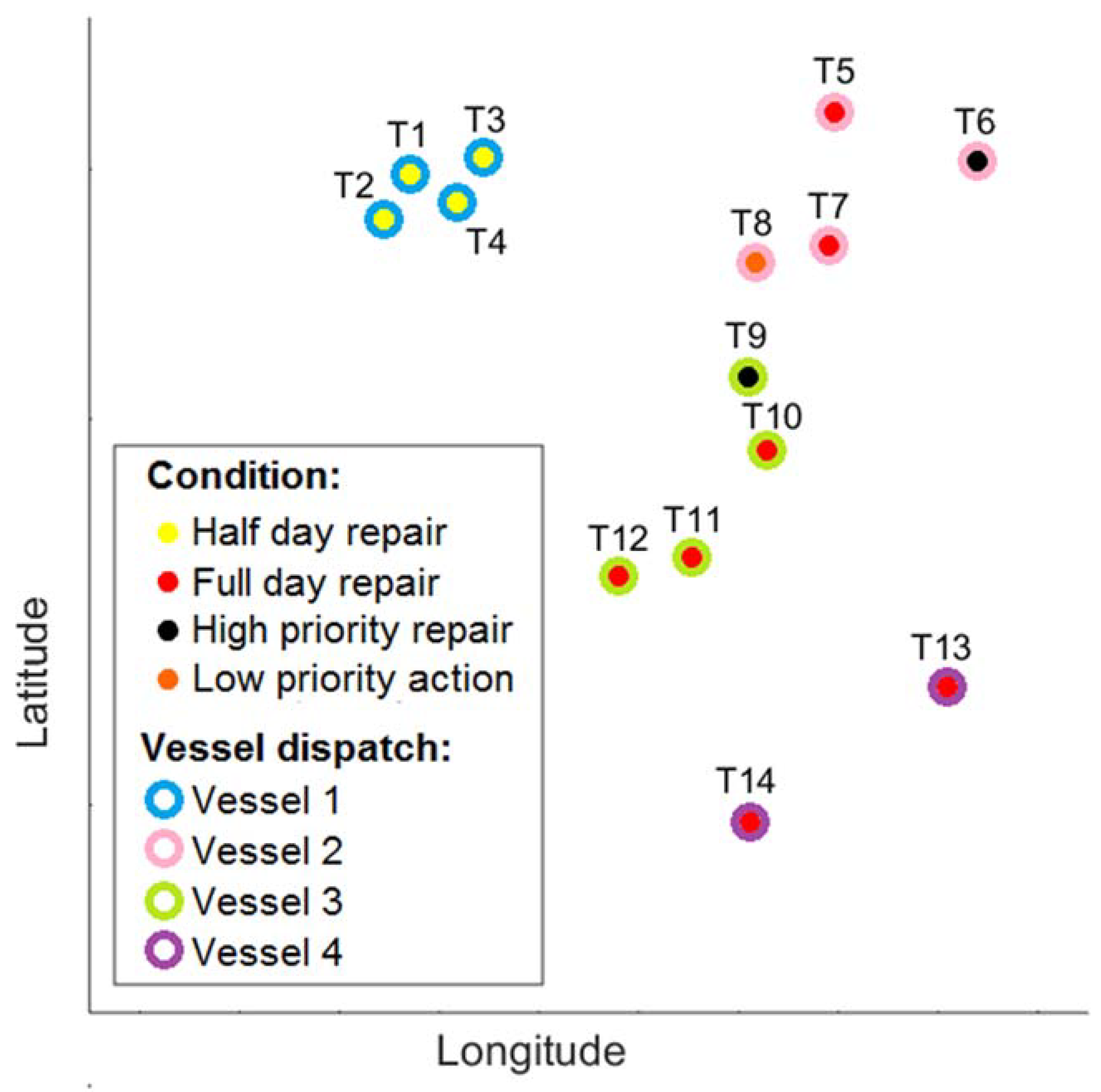
To aid the validation process of the tool developed in this paper, a visit to an operations centre of a large North Sea offshore wind farm was arranged. The real-life scenario presented in this section is less complex than the problem shown in Case Study 1; there are fewer faults, and the turbines are visibly clustered. While the purpose of Case Study 1 was to show the full capabilities of the tool and apply it to a complex, large problem, Case Study 2 was aimed at verifying the model’s assumptions and running the tool as the decisions were being made to find out whether the results produced are similar to policies created by the operators.
On a day in February 2017, 14 maintenance actions were set to be carried out. These can be divided into four categories:
- Half-day repairs, which tend to take around 2–3 h.
- Full day repairs, which tend to take around 5–7 h.
- High priority full day repairs involve turbines that have stopped generating power, and are to be visited as early as possible to maximise the time that technicians have on the turbine.
- Low priority maintenance actions, such as for example statutory tasks/inspections.
The properties of each repair type can be found in Table S6 in the Supplementary Material. High priority repairs were assigned a slightly longer maintenance action time and a higher value to ensure that they are visited before other repairs, while low priority actions were assigned a shorter maintenance action time and lower value.
The operators had five vessels available on the day, one of which was set aside to carry out auxiliary services on the wind farm, such as pre-loading spares and tools onto turbines. The properties of the remaining four vessels are shown in Table S7 in the Supplementary Material.
Uncertainties due to wave height, incorrect diagnosis, or repairs taking longer than expected were not taken into account in this case study; so, the risk aversion factor was set to 0. The weight of spares and tools was not a limitation on the day. The remaining model inputs can be found in Table S8 in the Supplementary Material. An overview of the maintenance actions to be carried out and the optimal policy selected by the tool are shown in Figure 6.
In terms of the assignment of vessels to turbines, the policy generated by the tool was the same as the decision made by the operators. The order in which crews were dropped off at turbines differed for two out of four vessels, as shown in Table 3. In both cases, the total distance travelled by the vessels was shorter in model-generated policies compared to the operators’ plan. However, the overall policy time would not differ by more than 10 min. The pick-up order was not compared as it is highly dependent on the time each crew finishes their activities; this decision is often made by the vessel captain rather than the operations team.
A number of practical considerations surfaced during the visit at the wind farm operations centre. These have not been modelled in the tool yet, but they may be of interest to researchers working on similar decision support tools for vessel routing for offshore wind farms:
- Operators tend not to assign one vessel to visit more than one turbine requiring high priority repair. Spreading crews carrying out these repairs across a number of vessels lowers the overall risk, as in some cases, due to unforeseen circumstances, a vessel may have to turn back to base before reaching the wind farm.
- It is preferred that certain maintenance actions are carried out by teams of three, although they can be completed by just two technicians if necessity arises.
- If a particular technician is assigned to travel on a vessel different to the one they were on the previous day, time has to be taken out of the overall time window to allow for craning their tools and equipment over.
Furthermore, the number of alarms and minor, non-critical maintenance actions on an offshore wind farm may be too large to input and update manually on a daily basis. The integration of a vessel routing decision support tool with the user’s alarm management system is crucial for successful practical application.
To the authors’ knowledge, this is the first publication in the academic domain in which a real-life problem of vessel routing for offshore wind farm was solved using mathematical modelling. The tool did not improve upon the policy created by the wind farm operators, but it could have helped make the decision more quickly. There may be scenarios in which the tool might outperform operators, such as for example when a larger number of maintenance actions are required, with more geographically dispersed repairs (such as Case Study 1). This practical case study has shown that the outputs of the tool developed here (assignment of vessels to turbines and the order in which turbines are visited) are similar to the decisions made by experienced wind farm operators.
4. Conclusions
The decision support tool described in this paper has the potential to reduce O&M costs by encouraging the effective use of resources in planning offshore logistics. The tool is capable of providing users with policies that are illustrated using a range of visual aids in short computational time.
To date, the research community working on vessel routing optimisation for offshore wind farms has failed to incorporate uncertainties into the decision-making process. The case study described in Section 3.1 shows that in the presence of uncertainties, the cost-optimal solution, which does not take into account uncertainties, will result in fewer turbines being successfully maintained. That a significant 14% increase in maintained turbines can be achieved by employing the proposed methodology highlights the importance of including uncertainties when modelling offshore vessel routing.
Allowing the user to specify risk aversion can facilitate tailoring policies to various scenarios. Increasing the risk aversion factor encourages policies that are more likely to be successfully completed. As Case Study 1 has shown, planning to visit fewer turbines can yield more successful repairs once uncertainties are taken into account.
The tool described in this paper was designed primarily for decision support. For a single scenario, multiple policies with varying risk aversion can be generated effortlessly. These choices can be discussed and evaluated by the vessel routing planners, allowing better decisions to be made. The automatically generated user-friendly outputs, which include policy plots and Gantt charts, help users visualise the proposed policies.
Consultations with wind farm operators enabled the validation of the tool’s assumptions and application of the tool to a real-life scenario. The tool’s outputs closely matched the decisions made by wind farm operators, showing that the model can transition from the theoretical domain into practical use. Furthermore, this publication adds value to the research domain by providing insight into real-life assumptions and practical considerations, helping other researchers formulate realistic case studies on which to test their models.
A number of improvements to the tool could be made with future work. These include the development of an algorithm for solving the problem of ordering turbine visits that are capable of assigning more than four turbines per vessel. Furthermore, the tool would benefit from the ability to distinguish different technician types and qualification levels. Future work will also include a computational study to investigate the effects of varying reward (Ui) inputs on the policies produced by the tool.
Supplementary Materials
A MS Word file and an MS Excel file containing input data referred to in the main body of this paper can be accessed at: http://dx.doi.org/10.15129/23f19557-8ede-4567-ac66-e4c838ca2cda.
Author Contributions
Conceptualization, R.D., D.M. and M.R.; Methodology, R.D., D.M. and M.R.; Software, R.D.; Validation, R.D.; Formal Analysis, R.D., D.M. and M.R.; Investigation, R.D., D.M. and M.R.; Resources, R.D., D.M. and M.R.; Data Curation, R.D.; Writing-Original Draft Preparation, R.D.; Writing-Review & Editing, R.D., D.M. and M.R.; Visualization, R.D.; Supervision, D.M. and M.R.; Project Administration, D.M. and M.R.; Funding Acquisition, R.D., D.M. and M.R.
Funding
This work was funded by Engineering Physical Sciences Research Council via the University of Strathclyde’s Wind Energy Systems Centre for Doctoral Training, grant number EP/G037728/1.
Conflicts of Interest
The authors declare no conflict of interest. The funders had no role in the design of the study; in the collection, analyses, or interpretation of data; in the writing of the manuscript, and in the decision to publish the results.
Abbreviation
| η | number of turbines in a cluster |
| A | risk aversion factor |
| a | shape parameter (Gamma distribution) |
| b | scale parameter (Gamma distribution) |
| Cfj | fuel cost for vessel j |
| Cri | cost of maintaining wind turbine i |
| Dk | number of technicians required to carry out maintenance on route k |
| E | number of technicians available |
| Fp | policy value (reward) |
| G | set of turbines (in a cluster/route) |
| i | turbine identifier |
| j | vessel identifier |
| K | set of feasible vessel routes |
| Ntj | number of turbines visited by vessel j |
| Pdi | probability of correct diagnosis of turbine i |
| Pri | probability of maintenance time at turbine i being less than the time available |
| Ptij | probability of successfully transferring crew from vessel j onto turbine i |
| Pvj | probability of vessel j being able to service all maintenance tasks assigned to it |
| Qk | binary decision variable (whether route k is selected) |
| Ri | expected maintenance time at turbine i |
| Sik | binary parameter (whether turbine i is on route k) |
| Ui | reward for maintaining turbine i |
| Vkj | binary parameter (whether vessel j is assigned to route k) |
| Xi | time available for maintenance atcions at turbine i |
| Y | critical path slack time |
| Z | non-critical path slack time |
References
- Ho, A.; Mbistrova, A. The European Offshore Wind Industry: Key Trends and Statistics 2016. Available online: https://windeurope.org/wp-content/uploads/files/about-wind/statistics/WindEurope-Annual-Offshore-Statistics-2016.pdf (accessed on 25 July 2018).
- The Crown Estate. Offshore Wind Cost Reduction: Pathways Study. Available online: https://www.thecrownestate.co.uk/media/5493/ei-offshore-wind-cost-reduction-pathways-study.pdf (accessed on 29 May 2017).
- Newman, M. Operations and Maintenance in Offshore Wind: Key Issues for 2015/16, Report by ORE Catapult. Available online: https://pdfs.semanticscholar.org/93ac/c7c22b705811c153679ee49d8f256ae21f77.pdf (accessed on 29 August 2018).
- Irawan, C.A.; Ouelhadj, D.; Jones, D.; Stålhane, M.; Sperstad, I.B. Optimisation of maintenance routing and scheduling for offshore wind farms. Eur. J. Oper. Res. 2017, 256, 76–89. [Google Scholar] [CrossRef] [Green Version]
- Dai, L.; Stålhane, M.; Utne, I.B. Routing and Scheduling of Maintenance Fleet for Offshore Wind Farms. Wind Eng. 2014, 39, 15–30. [Google Scholar] [CrossRef]
- Zhang, Z. Scheduling and Routing Optimization of Maintenance Fleet for Offshore Wind Farms using Duo-ACO. Adv. Mater. Res. 2014, 1039, 294–301. [Google Scholar] [CrossRef]
- Stålhane, M.; Hvattum, L.M.; Skaar, V. Optimization of Routing and Scheduling of Vessels to Perform Maintenance at Offshore Wind Farms. Energy Proc. 2015, 80, 92–99. [Google Scholar] [CrossRef]
- Caceres-Cruz, J.; Pol, A.; Guimarans, D.; Riera, D.; Juan, A.A. Rich Vehicle Routing Problem: Survey. ACM Comput. Surv. 2014, 47, 1–28. [Google Scholar] [CrossRef]
- Shafiee, M. Maintenance logistics organization for offshore wind energy: current progress and future perspectives. Renew. Energy 2015, 77, 182–193. [Google Scholar] [CrossRef]
- Dawid, R.; McMillan, D.; Revie, M. Development of an O&M Tool for Short Term Decision Making Applied to Offshore Wind Farms. Available online: https://www.researchgate.net/publication/312970476_Development_of_an_OM_tool_for_short_term_decision_making_applied_to_offshore_wind_farms (accessed on 14 May 2018).
- IBM ILOG CPLEX Optimization Studio V12.6.1 User Manual. Available online: https://www.ibm.com/support/knowledgecenter/SSSA5P_12.6.1/ilog.odms.studio.help/Optimization_Studio/topics/COS_home.html (accessed on 20 August 2018).
- Sun, L.; Wang, B. Robust Optimisation Approach for Vehicle Routing Problems with Uncertainty. Math. Probl. Eng. 2015, 2015. [Google Scholar] [CrossRef]
- Allahviranloo, M.; Chow, J.Y.J.; Recker, W.W. Selective vehicle routing problems under uncertainty without recourse. Transp. Res. Part E 2014, 62, 68–88. [Google Scholar] [CrossRef]
- Moghaddam, B.; Ruiz, R.; Sadjadi, S. Computers & Industrial Engineering Vehicle routing problem with uncertain demands: An advanced particle swarm algorithm. Comput. Ind. Eng. 2012, 62, 306–317. [Google Scholar]
- Marinakis, Y.; Iordanidou, G.; Marinaki, M. Particle Swarm Optimization for the Vehicle Routing Problem with Stochastic Demands. Appl. Soft Comput. J. 2013, 13, 1693–1704. [Google Scholar] [CrossRef]
- Tas, D.; Dellaert, N.; Woensel, T.V.; Kok, T.D. Vehicle routing problem with stochastic travel times including soft time windows and service costs. Comput. Oper. Res. 2013, 40, 214–224. [Google Scholar] [CrossRef] [Green Version]
- Russell, R.A.; Urban, T.L. Vehicle routing with soft time windows and Erlang travel times. Oper. Res. Soc. 2008, 59, 1220–1228. [Google Scholar] [CrossRef]
- Oyola, J.; Arntzen, H.; Woodruff, D.L. The stochastic vehicle routing problem, a literature review, part I: models. EURO J. Transp. Logist. 2016. [Google Scholar] [CrossRef]
- Li, X.; Tian, P.; Leung, S.C.H. Vehicle routing problems with time windows and stochastic travel and service times: Models and algorithm. Int. J. Prod. Econ. 2010, 125, 137–145. [Google Scholar] [CrossRef]
- Lei, H.; Laporte, G.; Guo, B. A generalized variable neighborhood search heuristic for the capacitated vehicle routing problem with stochastic service times. J. Span. Soc. Stat. Oper. Res. 2012, 20, 99–118. [Google Scholar] [CrossRef]
- Chen, L.; Hoàng, M.; Langevin, A.; Gendreau, M. Optimizing road network daily maintenance operations with stochastic service and travel times. Transp. Res. Part E 2014, 64, 88–102. [Google Scholar] [CrossRef]
- Gómez, A.; Mariño, R.; Akhavan-Tabatabaei, R.; Medaglia, A.L.; Mendoza, J.E. On Modeling Stochastic Travel and Service Times in Vehicle Routing. Transp. Sci. 2016, 50, 627–641. [Google Scholar] [CrossRef]
- Bertsimas, D.J.; van Ryzin, G. Stochastic and Dynamic Vehicle Routing with General Demand and Interarrival Time Distributions. Adv. Appl. Probab. 1993, 25, 947–978. [Google Scholar] [CrossRef]
- Chepuri, C.; Homem-De-Mello, T. Solving the vehicle routing problem with stochastic demands and customers. Ann. Oper. Res. 2005, 153–181. [Google Scholar] [CrossRef]
- Dawid, R.; McMillan, D.; Revie, M. Time Series Semi-Markov Decision Process with Variable Costs for Maintenance Planning. Available online: https://strathprints.strath.ac.uk/58070/1/Dawid_etal_Esrel2016_Time_series_semi_markov_ decision_process.PDF (accessed on 25 July 2018).
- Dinwoodie, I.; Endrerud, O.-E.V.; Hofmann, M.; Martin, R.; Sperstad, I.B. Reference Cases for Verification of Operation and Maintenance Simulation Models for Offshore Wind Farms. Wind Eng. 2015, 39, 1–14. [Google Scholar] [CrossRef] [Green Version]
Figure 1.
Outline of the model’s structure.

Figure 2.
A map of wind turbine locations and maintenance actions required.
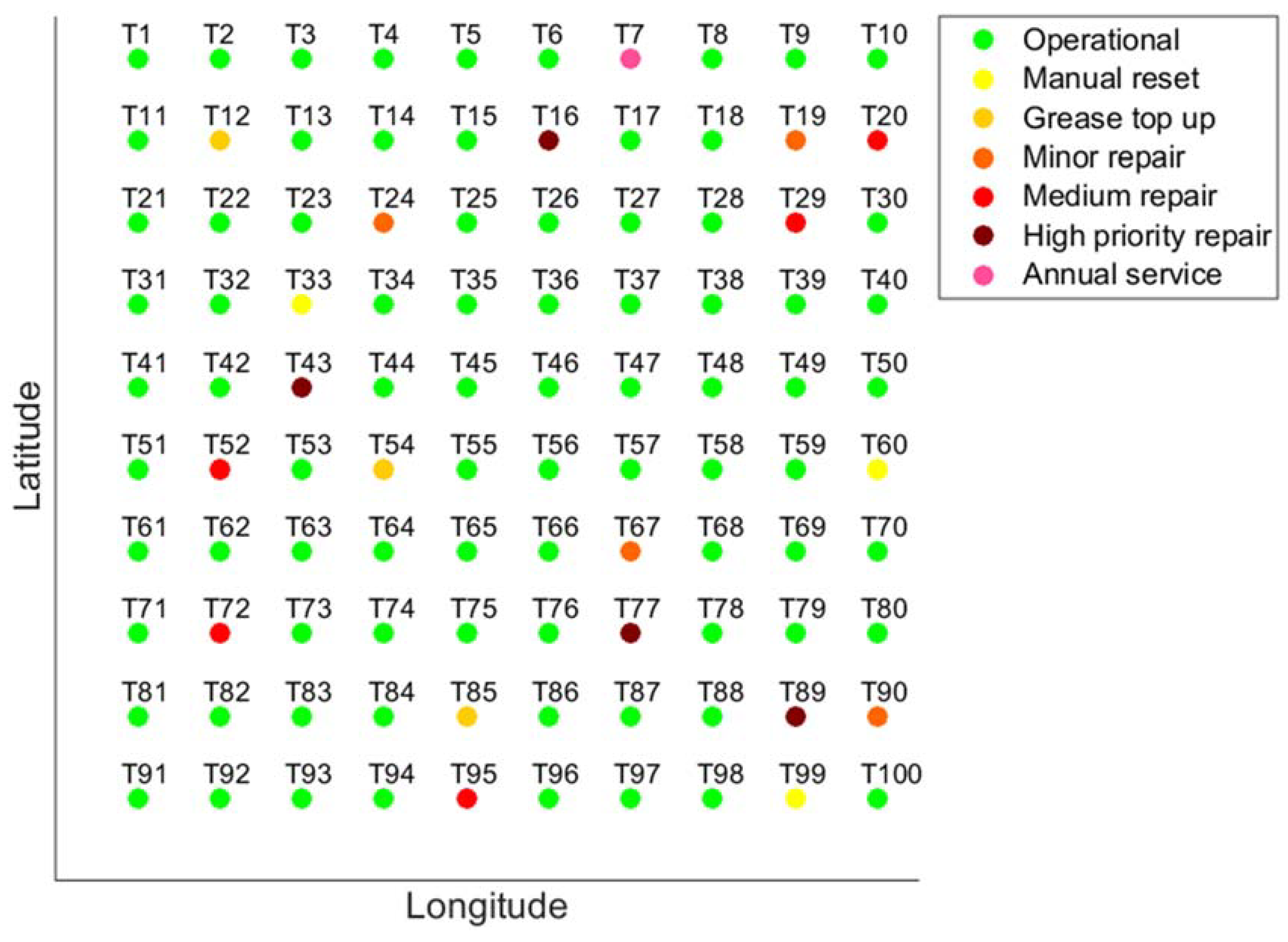
Figure 3.
Vessel dispatch plan for Case 1. This figure, with arrows indicating individual vessel movements, is shown in Figure S2 in the Supplementary Material.
Figure 3.
Vessel dispatch plan for Case 1. This figure, with arrows indicating individual vessel movements, is shown in Figure S2 in the Supplementary Material.
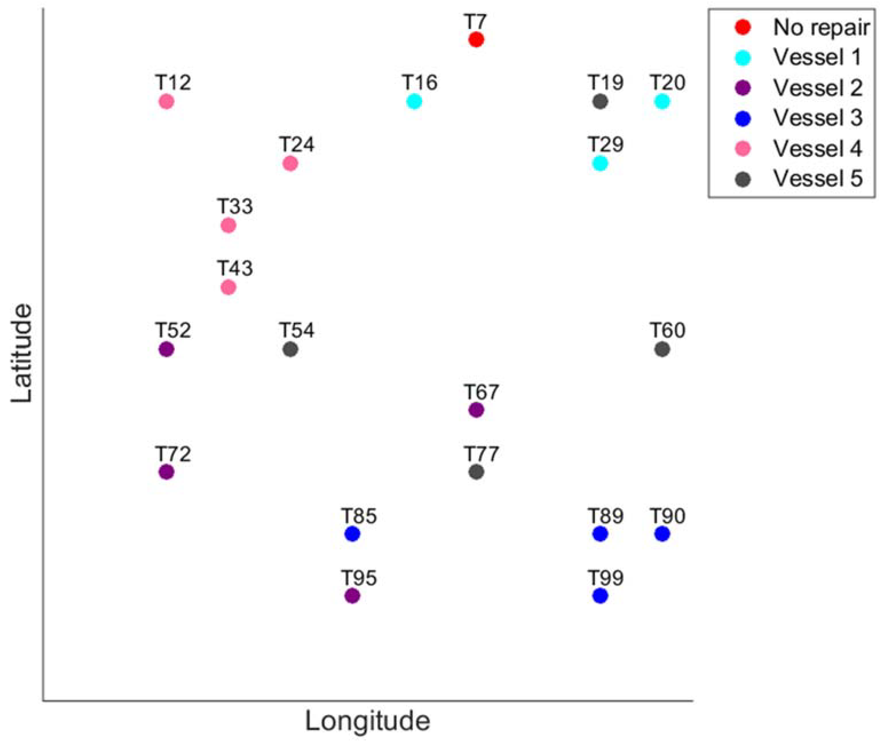
Figure 4.
Vessel dispatch plan for Case 3.
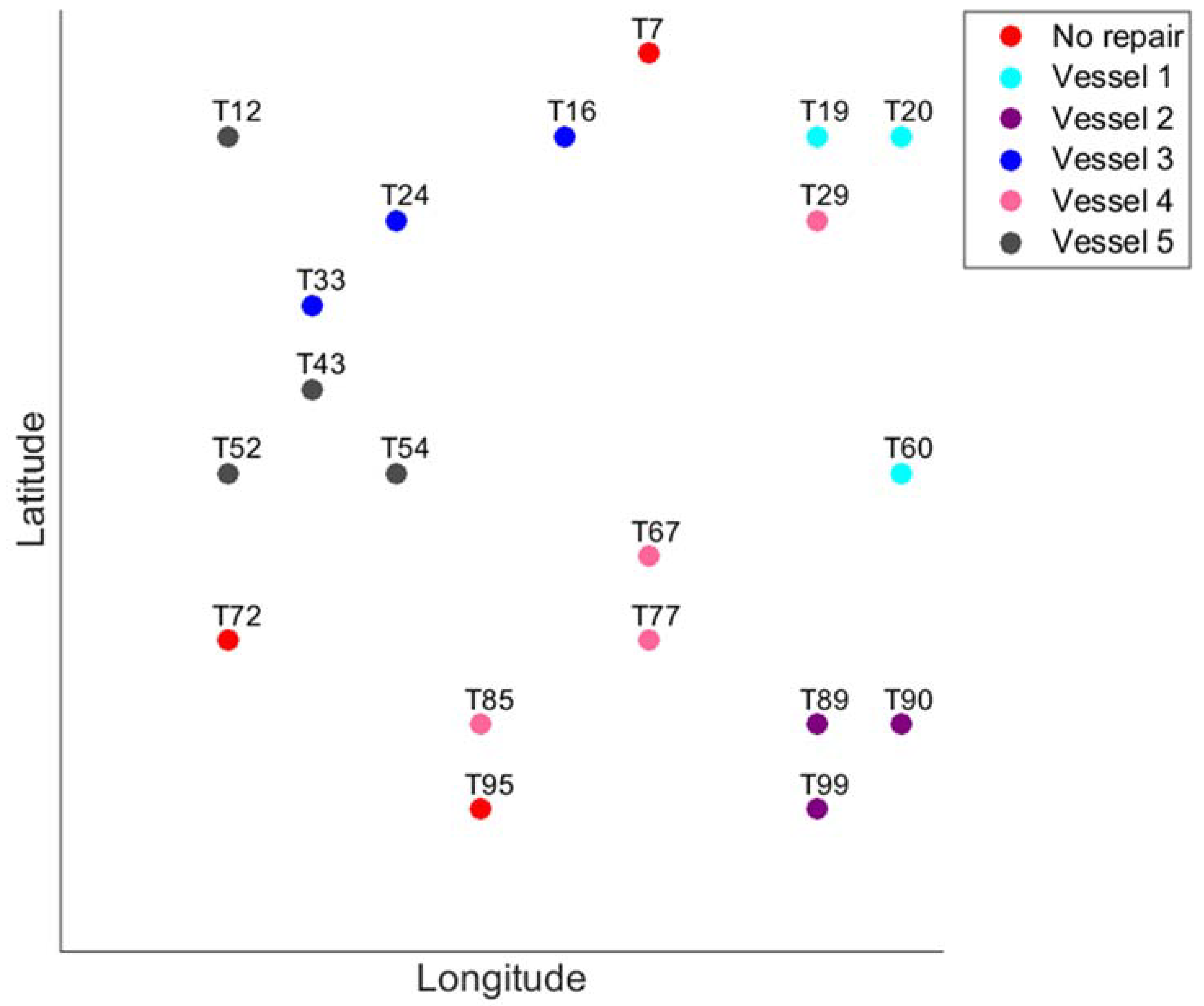
Figure 5.
Breakdown of the Monte Carlo analysis for cases 1–5. Note that increasing the risk aversion factor favours less ‘risky’ policies.
Figure 5.
Breakdown of the Monte Carlo analysis for cases 1–5. Note that increasing the risk aversion factor favours less ‘risky’ policies.

Figure 6.
The status of turbines requiring maintenance and a vessel dispatch plan for Case Study 2.

Table 1.
Comparison of cases including Monte Carlo simulation results.
| Policy Characteristics | Case 1 | Case 2 | Case 3 | Case 4 | Case 5 |
|---|---|---|---|---|---|
| Risk aversion factor (A) | 0 | 2.5 | 5 | 7.5 | 10 |
| Planned number of turbines to be maintained (/20) | 19 | 18 | 17 | 16 | 14 |
| Planned number of high priority turbines to be maintained (/4) | 4 | 4 | 4 | 4 | 4 |
| Expected policy value (not including value added due to a non-zero A) (£ ,000) | 1685.1 | 1603.3 | 1522.5 | 1440.7 | 1277.9 |
| Number of technicians required to carry out all of the maintenance actions | 45 | 44 | 45 | 40 | 34 |
| From Monte Carlo simulation (as described in Section 3.2): | |||||
| Average number of turbines actually maintained (/20) | 10.8 | 10.8 | 12.1 | 11.1 | 11.5 |
| Turbines not maintained due to actions taking longer than expected | 5.6 | 4.9 | 3.1 | 3 | 1.3 |
| Turbines not maintained due to unsuccessful transfer | 1.2 | 1 | 0.6 | 0.8 | 0.2 |
| Turbines not maintained due to incorrect diagnosis | 1.4 | 1.3 | 1.2 | 1.1 | 1 |
Table 2.
Suggested order of visits for cases 1 and 3.
| Case | Vessel | Probability | Tech. Crews | Turbines Visited | Order of Visits | |||||||
|---|---|---|---|---|---|---|---|---|---|---|---|---|
| Case 1 | Vessel 1 | 20.2% | 3 | 3 | T20 | T29 | T16 | T16 | T20 | T29 | ||
| Vessel 2 | 9.8% | 4 | 4 | T52 | T72 | T95 | T67 | T67 | T52 | T72 | T95 | |
| Vessel 3 | 18.5% | 3 | 4 | T85 | T89 | T90 | T85 | T99 | T90 | T89 | T99 | |
| Vessel 4 | 19.3% | 3 | 4 | T12 | T43 | T24 | T12 | T33 | T24 | T43 | T33 | |
| Vessel 5 | 17.3% | 3 | 4 | T54 | T77 | T19 | T54 | T60 | T19 | T77 | T60 | |
| Case 3 | Vessel 1 | 53.3% | 3 | 3 | T20 | T19 | T60 | T60 | T19 | T20 | ||
| Vessel 2 | 54.3% | 3 | 3 | T89 | T90 | T99 | T99 | T90 | T89 | |||
| Vessel 3 | 44.8% | 3 | 3 | T16 | T24 | T33 | T33 | T24 | T16 | |||
| Vessel 4 | 12.4% | 4 | 4 | T29 | T77 | T67 | T85 | T85 | T67 | T77 | T29 | |
| Vessel 5 | 14.4% | 4 | 4 | T52 | T43 | T54 | T12 | T54 | T12 | T43 | T52 | |
Table 3.
Comparison of the policy devised by the operators vs. generated by the tool.
| Vessel | Order Source | Drop-Off Order | Difference in Distance Travelled (km) | |||
|---|---|---|---|---|---|---|
| Vessel 1 | Actual | 2 | 4 | 3 | 1 | 0.42 |
| Tool | 3 | 2 | 4 | 1 | ||
| Vessel 2 | Actual | 6 | 5 | 7 | 8 | 0 |
| Tool | 6 | 5 | 7 | 8 | ||
| Vessel 3 | Actual | 9 | 11 | 12 | 10 | 3.58 |
| Tool | 9 | 10 | 11 | 12 | ||
| Vessel 4 | Actual | 13 | 14 | 0 | ||
| Tool | 13 | 14 | ||||
© 2018 by the authors. Licensee MDPI, Basel, Switzerland. This article is an open access article distributed under the terms and conditions of the Creative Commons Attribution (CC BY) license (http://creativecommons.org/licenses/by/4.0/).
Share and Cite
MDPI and ACS Style
Dawid, R.; McMillan, D.; Revie, M. Decision Support Tool for Offshore Wind Farm Vessel Routing under Uncertainty. Energies 2018, 11, 2190. https://doi.org/10.3390/en11092190
AMA Style
Dawid R, McMillan D, Revie M. Decision Support Tool for Offshore Wind Farm Vessel Routing under Uncertainty. Energies. 2018; 11(9):2190. https://doi.org/10.3390/en11092190
Chicago/Turabian StyleDawid, Rafael, David McMillan, and Matthew Revie. 2018. "Decision Support Tool for Offshore Wind Farm Vessel Routing under Uncertainty" Energies 11, no. 9: 2190. https://doi.org/10.3390/en11092190
Note that from the first issue of 2016, this journal uses article numbers instead of page numbers. See further details here.