Coordinated Control for Large-Scale Wind Farms with LCC-HVDC Integration


1
Department of Automation, Tsinghua University, Beijing 100084, China
2
State Power Economic Research Institute, State Grid Corporation of China, Beijing 102209, China
*
Author to whom correspondence should be addressed.
Energies 2018, 11(9), 2207; https://doi.org/10.3390/en11092207
Submission received: 30 July 2018
/
Revised: 19 August 2018
/
Accepted: 21 August 2018
/
Published: 23 August 2018
(This article belongs to the Special Issue Power Quality in Microgrids Based on Distributed Generators)
Abstract
:Wind farms (WFs) controlled with conventional vector control (VC) algorithms cannot be directly integrated to the power grid through line commutated rectifier (LCR)-based high voltage direct current (HVDC) transmission due to the lack of voltage support at its sending-end bus. This paper proposes a novel coordinated control scheme for WFs with LCC-HVDC integration. The scheme comprises two key sub-control loops, referred to as the reactive power-based frequency (Q-f) control loop and the active power-based voltage (P-V) control loop, respectively. The Q-f control, applied to the voltage sources inverters in the WFs, maintains the system frequency and compensates the reactive power for the LCR of HVDC, whereas the P-V control, applied to the LCR, maintains the sending-end bus voltage and achieves the active power balance of the system. Phase-plane analysis and small-signal analysis are performed to evaluate the stability of the system and facilitate the controller parameter design. Simulations performed on PSCAD/EMTDC verify the proposed control scheme.
1. Introduction
The power system is facing unprecedented technical challenges due to abundant large-scale renewable power plant integration [1,2,3,4,5]. In China, large-scale wind farms (WFs) are mainly built in remote areas of the northwest. As the local alternating current (AC) network is quite weak and the penetration level of wind power is extremely high, it is a critical technical issue to integrate and deliver large-scale wind power into the southeastern power grid. Emerging ultra HVDC (UHVDC) transmission technology is able to provide an available solution. To date, most of the UHVDC systems that are being planned or that are already built are of the line commutated converter (LCC) type, which are suitable for long-distance and large-capacity transmission, with advantages such as low expenditure and power loss [4]. Recently, a ±800 kV UHVDC with 10 GW capacity is being planned to deliver wind and solar power on the Tibetan Plateau into the eastern load center, and wind and solar power accounts for about 85% of the transmission capacity. It is quite difficult for the system to maintain stable operation when there is no traditional generating set that is available at the sending end of the UHVDC, due to some special factors, e.g., circuit faults, but only islanded WFs and/or photovoltaic power plants. Therefore, it is necessary to study the control scheme of large-scale WFs with LCC-HVDC integration as a technical reserve [4,5,6,7].
Vector control (VC) algorithms are commonly used for the control of wind energy conversion systems (WECSs). Conventional VC [8] is based on the orientation of the grid voltage vector, and thus a stiff grid is required to ensure the stability of the systems [9]. Unlike the voltage source converter in VSC-HVDC, the line commutated rectifier (LCR) in LCC-HVDC cannot actively generate the referenced three-phase voltage, essentially because of the application of semi-controlled switching devices, e.g., thyristors. Moreover, a steady and balanced commutation voltage is a prerequisite for the operation of the LCR. Consequently, under the condition that there is no available voltage support at the sending-end bus (SEB) of LCC-HVDC, the WFs with conventional VC algorithms cannot can be integrated by the LCC-HVDC directly [10,11,12].
A simple approach is to introduce a static synchronous compensator (STATCOM) on the SEB in order to provide the voltage support [10,11,12]. However, the extremely high reliability and large capability is required for the STATCOM, which results in high operating costs and power loss [13]. Without voltage support, the critical issue in the system is to guarantee the stability of the SEB voltage vector, including both the voltage stability and the frequency stability. Considering that the LCR is controllable in terms of active power, both the frequency and voltage stability issues can be addressed through the division of labor between the WF and the LCR [14,15,16,17,18,19], i.e., the voltage and the frequency are controlled by the WF and the LCR respectively, or conversely.
For the doubly-fed induction generator (DFIG)-based offshore WF at steady states, the stator voltage of the DFIG is the product of its stator flux and the SEB frequency [14]. Based on this fact, the earliest approach, where the stator flux and the frequency are controlled by the WF and the LCR respectively, is proposed in [14,15]. A similar approach can be found in [16], where the stator voltage and the frequency are controlled by the WF and the LCR respectively. In both of the approaches, the frequency is regulated by the active power of the WF, whereas the voltage is regulated by the reactive power of the WF. Actually, there is a substantial amount of capacitive compensation on the SEB of the LCC-HVDC or diode-based HVDC, leading to a strong coupling between the bus voltage and the active power balance, and also between the frequency and the reactive power balance [17,20,21,22]. Consequently, references [17,20,21,22] develop a novel control concept, where the frequency is regulated by the reactive power, whereas the voltage is regulated by the active power. There is another coordination approach developed in [18,19] where the voltage is controlled by both the WF and the LCR. As a result, the strong coupling between the active and reactive power control loops occurs, which would affect the dynamic performance of the system. Moreover, the frequency stability was not addressed in the approach.
In the aforementioned approaches, the control algorithms of the WFs are based on the conventional VC structure where phase-locked loops (PLLs) are employed to detect the phase-angle of the stator voltage. It is reported that PLLs play an important role in the system dynamics, and the system stability involving PLLs are quite complicated [9], especially when WFs are connected to the weak, or even isolated grids [23,24]. There are some intensive studies regarding the PLL-less DFIG control algorithms for standalone applications, referred to as the indirect self-orientated vector control (ISOVC) [25,26,27,28]. In the ISOVC, the phase-angle, adopted in the coordinate transformation between abc and dq reference frames, is derived from a free running integral of the rated synchronous speed ω0 instead of the PLL. It is worth noting that the supplementary indirect orientation control is realized through modifying the original active power loop, and thus the auxiliary torque and pitch angle control is required to regulate the active power [25,26,27,28]. Since the probability of frequency instability due to the dynamic characteristics of PLLs can be completely avoided in the ISOVC, it is applied to control standalone DFIGs with LCC-HVDC integration in [29]. In order to be employed in multi-machine scenarios, additional active power droop loop should be introduced into ω0 to achieve synchronization and power sharing among multiple machines [29,30]. Unfortunately, with such droop scheme, the WF cannot always track its maximum power point with sacrificed economic benefits.
In this paper, a novel scheme with respect to the division of labor between the WF and the LCR is proposed. On one hand, considering the coupling relationship between the frequency and the reactive power balance [17,18,19,20], a novel indirect orientation control based on the reactive power loop instead of the active power loop [25,26,27,28] is developed. In the scheme, reactive power droop is employed for synchronization and reactive power sharing among multiple machines. Therefore, it would not affect the active power tracking of the WF. On the other hand, the control objective of the LCR is to maintain the SEB voltage stability. Actually, since there is a strong coupling between the voltage and the active power balance, not only can the voltage stability be addressed, but also the WF is able to capture the maximum active power with the proposed scheme. The proposed scheme comprises two key sub-control loops. One is the reactive power-based frequency (Q-f) control loop for the voltage source inverters (VSIs) in the WF, where a novel ISOVC is developed to maintain the SEB frequency and compensate reactive power for the LCR. The other is the active power-based voltage (P-V) control loop for the LCR, through which the SEB voltage is controlled to achieve the active power balance.
The rest of the paper is organized as follows. Section 2 depicts the mathematical models, and explains the relationship between the voltage and the active power balance, and also between the frequency and the reactive power balance. Section 3 proposes the Q-f and P-V control loops after analyzing the operational principles. Section 4 demonstrates the stability of the proposed control scheme and designs the controller parameters. Section 5 shows the simulation results and verifies the feasibility of the coordinated control scheme. Section 6 concludes this paper.
2. System Modeling
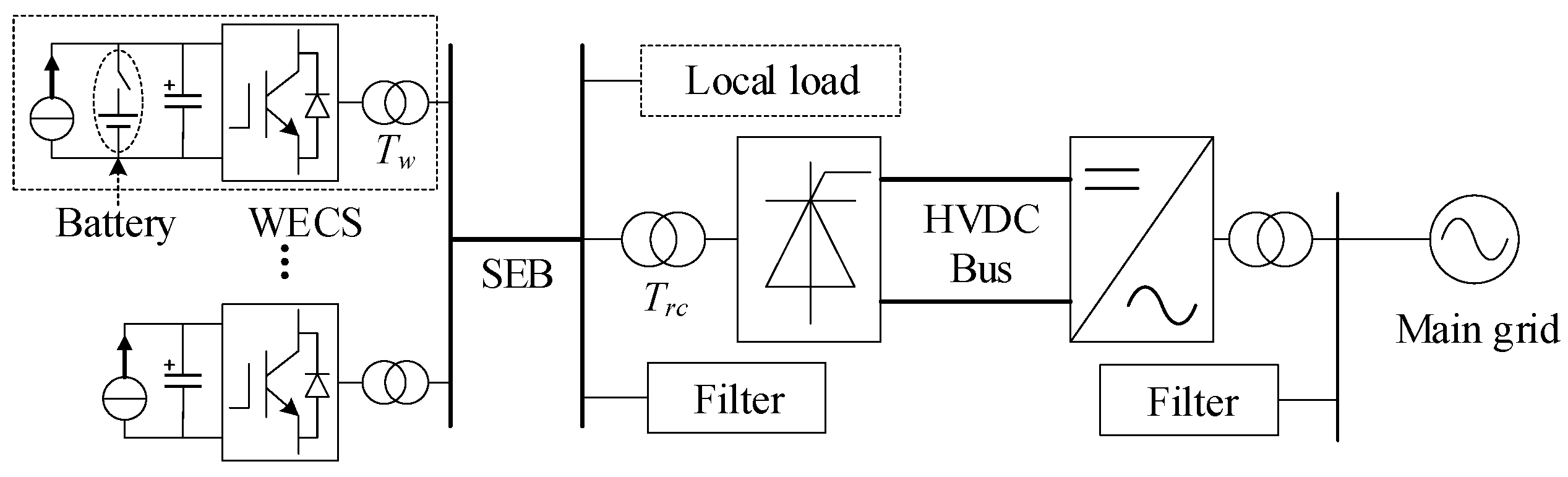
The topology of the studied system is shown in Figure 1. This study takes permanent-magnet synchronous generator (PMSG)-based WECSs as an example to study the coordination between WFs and LCC-HVDC. The proposed control scheme can be easily extended to doubly-fed induction generator (DFIG)-based WECSs. It should be noticed that the Q-f control is applied in grid-side VSIs of PMSG-based WECSs, whereas it is applied in rotor-side converters of DFIG-based WECSs. For simplicity, the PMSG-based WECS can be equivalent to a voltage source inverter (VSI) in parallel with a direct current (DC) capacitor and a controlled DC current source [31]. In order to supply energy for the system startup, batteries are installed at the DC bus of several units (no need for all units). Especially, for the DFIG-based WECSs, rotor excitation of DFIGs should be provided initially in the startup process, which can be accomplished through the rotor-side converters powered by the batteries. The WECSs are connected to the SEB of HVDC. The rectifier is of the LCC type, and thus a substantial amount of AC filters are configured at the SEB to mitigate the current harmonics, and meanwhile they provide reactive power compensation, which can be equivalent to a capacitor bank Cf at the fundamental frequency.
For a clear description of the system model, it can be divided into three subsystems: the WECS subsystem, the SEB subsystem and the HVDC subsystem. To capture the fundamental power dynamic characteristics of the system, the switching function models [10,11] of the converters are employed. Moreover, the inverter of HVDC can be equivalent to a DC voltage source [14,15] since it is subjected to a constant-voltage control and has little effect on the other subsystems under normal operations. Figure 2 depicts the equivalent circuit of the whole system, where the significations of the electrical variables and parameters are self-explanatory.
2.1. WECS Subsystem Model
In the rated synchronous reference frame (RSEF) with the rated frequency ω0, the WECS model can be written as:
where the subscripts d and q represent the variables transformed from the three-phase abc reference frame to the dq RSEF, and ωb is the base frequency, similarly hereinafter.
2.2. SEB Subsystem Model
Similarly, the SEB model in the RSEF can be written as:
Let the amplitude and the phase-angle of the SEB voltage be:
It can be obtained in the polar coordinate system that [19,20]:
where Pw = ubdiwd + ubqiwq and Prc = ubdircd + ubqircq are the active powers from the WECS, and they are absorbed by the HVDC respectively. Also, Qw = –ubdiwq + ubqiwd and Qrc = –ubdircq + ubqircd are the reactive powers from the WECS and they are absorbed by the LCR respectively, and ω1 is the SEB frequency.
Equations (5) and (6) lay the foundations for this study. From the perspective of the filter capacitor parallel branch, the WECS can be seen as a controlled power source (Pw and Qw), while the LCR can be seen as a controlled power load (Prc and Qrc). Given that the WECS and the HVDC are interconnected by the filter capacitor, two significant results can be drawn from the filer capacitor point of view. (1) The voltage amplitude Ubm is highly coupled with the active power (Pw − Prc); (2) The phase-angle (or the frequency ω1) is highly coupled with the reactive power (Qw − Qrc) [20]. A physical mechanism explanation is given as follows.
It is known that the total instantaneous power of the three-phase balanced capacitor branch equals its active power (which is zero) at steady states, and the power exchanged within the three-phase capacitors charges/discharges the capacitors. As a result, the three-phase capacitor circuit as a whole exhibits a certain reactive power. However, this conclusion becomes invalid during dynamic processes. For Equation (5), if there is an active power deviation, e.g., Pw − Prc > 0, this indicates that the active power generated by the WECS is larger than that absorbed by the LCR, then the extra active power will charge the capacitors. Consequently, the instantaneous current amplitude will increase, which leads the instantaneous voltage amplitude to increase too. Similarly, if there is a reactive power deviation for Equation (6), e.g., (–Qw + Qrc) > 0, which indicates that the reactive power generated by the WECS is smaller than that absorbed by the LCR, then the voltage phase-angle (i.e., the instantaneous frequency) will increase, assuming that the voltage amplitude keeps unchanged. As a consequence, the capacitive reactance will decrease due to the frequency increase, and therefore the capacitor will generate more reactive power to try to balance the reactive power. In fact, the capacitive parallel branch is in a dual relationship with the inductive series branch in traditional power systems, and thus it is not difficult to understand the foregoing coupling relationship. Moreover, it can be also found that a smaller Cf (the absolute minimum filter guarantees Cf > 0) can result in a stronger coupling.
2.3. HVDC Subsystem Model
In the RSEF, the HVDC model can be written as [11,12]:
where α is the firing angle, and Urcm is the voltage amplitude in the rectifier bridge side. Note that the variables are in the per-unit system, and thus the rectifier coefficient is eliminated. Also, both the (12k ± 1) order harmonics in ac side and the 12k order harmonics in DC side are neglected in the typical 12-plus HVDC model, since the events of major concern are the fundamental power conversion rather than high frequency dynamic.
3. Coordinated Control Scheme
Prior to describing the proposed coordinated control scheme, the control requirements should be emphasized first.
- (1)
- Voltage control: a stable voltage can offer voltage support for the WECSs, as well as the commutation voltage for the LCR.
- (2)
- Frequency control: the frequency stability should be maintained so that multiple WECSs are able to operate synchronously.
- (3)
- Active power balance: considering that the wind conditions are not controlled, the active power generated from the WFs should be equal to that which is transmitted into the HVDC in real time.
- (4)
- Reactive power balance: considering that the reactive power compensation capability of AC filters is discontinuous, the WECSs should be able to compensate and share the insufficient or excessive reactive power automatically.
The proposed coordinated control scheme is able to achieve the requirements. The Q-f control applied into the wind farm meets the requirements (2) and (4), whereas the P-V control applied into the HVDC rectifier meets the requirement (1) and (3). Thus, the wind farm and the HVDC cooperate with each other to achieve system stability.
Note that the resynchronization capability is also of much significance for the system uninterrupted operation in the case of a fault. Under fault conditions, the back-end converters can be controlled to supply zero power temporarily, and then the batteries can be utilized again to help generate the SEB voltage after the fault is cleared. More technical details will be given in future work.
3.1. Q-f Control of WECSs
In contrast to the ISOVC in [25,26,27,28], where the active power loop is adopted to achieve indirect orientation and synchronization, a novel ISOVC will be developed here. Since that the relationship between the frequency and reactive power, as shown in Equation (6), the reactive power loop is adopted to achieve Q-f control. As depicted in Figure 3, two key modifications are made in the Q-f control compared with the conventional VC with the unity power factor. One is that the self-defined phase-angle is:
where ∠0 is an initial value, determined by the final value of the phase-angle at the end of system startup. The other is that the control object of the reactive power loop is regulating the q-axis voltage ubq instead of the reactive current iwq to zero. As a consequence, not only is the frequency ω1 clamped when ubq = 0 since the actual phase-angle is consistent with the self-defined one, but the reactive current command iwq* can also be regulated automatically so that the WECS is able to compensate reactive power for the LCR. Note that the active power control is still based on the maximum power point tracking (MPPT) control, as shown in Figure 3b. The operational principle of the Q-f control is described as follows.
Assuming that the system is in a steady state, if the frequency ω1 suddenly starts to increase due to a disturbance, e.g., a sudden increase of the reactive power Qrc, the voltage vector Ub and current vector Iw under conventional VC is shown in Figure 4a. It can be observed that the controller tracks the frequency change and cannot output the reactive power to regulate the frequency, which further leads to the instability of frequency. In Figure 4b, the self-oriented control (11) is adopted, but the reactive power loop still regulates iwq to zero. Under this condition, Ub rotates counterclockwise an angle ϕ due to the increase of frequency. Thus, although the WECS outputs reactive power, Ub no longer coincides with the q-axis because of a lack of synchronization control. Thereafter, the d- and q-axis controls are no longer decoupled, and moreover, multiple WECSs may become asynchronous due to the accumulation of the angle errors. In Figure 4c, the issue is completely addressed where the control object is ubq = 0 instead of iwq = 0. In other words, the phase-angle is indirectly controlled to follow the angle generated by the rated frequency ω0, and the controller output signal is exactly the reactive current reference. Consequently, the third proportional-integral (PI3) regulator is able to produce an exact reactive current reference iwq* under the condition that ubq = 0.
It should be noted that the PI3 regulator cannot work well in multi-WECS scenarios due to a reactive current circulation among the WECSs without a sharing scheme. To this end, a simple approach is to improve the PI-type regulator into a P-type one, resulting in a droop characteristic. Thus, when a multi-machine system is subjected to the Q-f droop control, the reactive power can be compensated and shared automatically, and both the frequency stability and the synchronization stability can be realized. With the P-type control, the voltage vector will no longer coincide with the d-axis. By defining an appropriate range of the included angle between them, and thereby setting an appropriate proportional coefficient, it is doable to ensure that the included angle is small enough and close to zero at steady states.
According to the P-type control, for one WECSj, it can be obtained that:
where ubqj can be considered to be approximately the same for different units. For one thing, in actual practice, ubqj = 0 at the time when WECSj switches from the pre-synchronization stage to the connection to the sending-end grid by means of phase-locked loops. For another, after the connection to the sending-end grid, the phase-locked loops are withdrawn. Then, the phase-angle difference between two units during normal operating conditions are also eliminated by their initial synchronous reference frames.
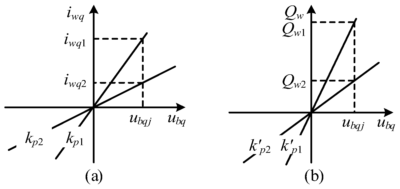
On the basis of Equation (12), the reactive power can be written as:
Figure 5 shows the droop curves of the reactive currents and the reactive powers with respect to the d-axis voltage. It can be observed in Figure 5a that a large proportional coefficient is able to result in a large shared reactive current. In Figure 5b, the sharing coefficient is given by Equation (13). Since the voltage vector and the d-axis are not strictly coincident, the reactive power is inevitably related to the active current iwdj. Even so, if a quite large kpj is taken, then the voltage vector and the d-axis will substantially coincide. In this point, it is known from Equation (13) that the reactive power contributed by the active current iwdj is relatively small. In short, the proportional coefficient of each unit can be calculated and designed based on Equation (13). In practical applications, the optimization control and the quantitative allocation of reactive power can be achieved considering the unit capacity limit. For example, a large proportional coefficient can be set for the unit with a small active power output so that it can share more reactive power.
In order to maintain the active power benefit of WFs, the active power priority principle can be adopted. As shown in Figure 3, according to the real-time active current iwd, the reactive current iwq is limited as follows:
Equation (14) defines the reactive power margin. There is no steady-state equilibrium point of reactive power, assuming that the reactive power demand exceeds the reactive power margin. Considering that the reactive power demand can be adjusted by the centralized reactive power compensation device, and that a WF has the minimum reactive power compensation capability, this study recommends the following reactive power compensation scheme: (1) For the entire WF, according to its rated capacity and maximum active power output to determine the minimum reactive power compensation capability. When the real-time reactive power output becomes larger than the minimum compensation capacity, the centralized reactive power compensation should be adjusted in time, such as the conventional filter or the high-performance static var compensator (SVC) or STATCOM. Consequently, the reactive power demand becomes smaller, and within the minimum compensation capability. (2) For each unit, according to its real-time active current, adjust the limitation of the reactive current according to Equation (14).
3.2. P-V Control of LCR
When the active power Pw from the WECS increases, it has been known that Ubm increases according to Equation (5) assuming that Prc remains constant. Actually, if Ubm increases, Prc will increase too. However, there is no doubt that the steady-state Ubm will become larger from the perspective of the whole circuit if the firing angle remains unchanged. Only if the LCR controller reduces the firing angle α, leading to more absorbed active power Prc by the LCR, can Ubm return back its reference value. A detailed analysis is performed as follows.
Based on the conclusions in [5], the time constant of the rectifier currents is quite small, about tens of milliseconds, under the constant-voltage control of the inverter of HVDC. Thus, the current transients in Equations (7) and (10) can be ignored while analyzing the active power balance, which gives rise to:
where Peq and Qeq are the active and reactive power of rectifier bridge, and δ is the phase-angle difference between Ub and Urc, and it can be seen as a power angle. Note that the internal resistor Rrc is ignored in Equation (15). Given that the power factor angle of the rectifier bridge (excluding Rrc and Lrc) is α, i.e.,:
Combining Equations (9), (10), (15), and (16), it can be obtained that:
Furthermore, considering the effect of the leakage inductor Lrc on the power factor angle of the LCR (including Trc), it exists as:
where Rc is the equivalent commutation resistor with an actual value 6/πω0Lrc. Substituting Equation (18) into Equations (9) and (10) yields that:
It can be assumed that both Ubm and udi remain constant under the controls of both the rectifier and inverter, and thus cos(δ + α) remains constant, according to Equation (17). Actually, when Pw increases, the power angle δ increases, whereas the firing angle α decreases along with the increase of id in Equation (19). Therefore, δ + α remains approximately unchanged. Since that δ + α is the power factor angle between Ub and Irc:
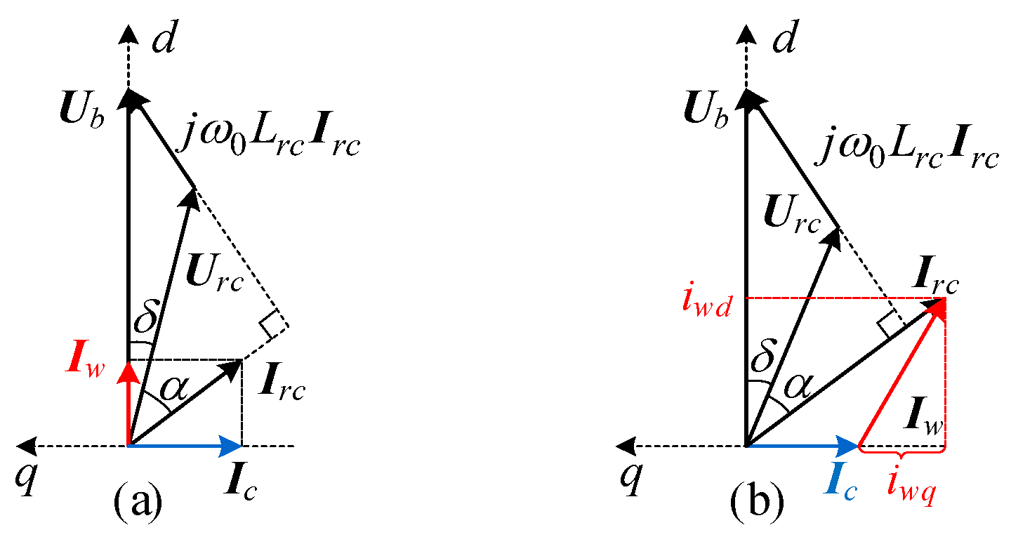
Let Ub be oriented to the d-axis of the rated synchronous reference frame (RSRF) (consistent with the orientation of the WECS), and the vector diagrams of the SEB is depicted in Figure 6. In Figure 6a, the active current iwd is smaller, and it can be assumed that the reactive current Ic from the filters can be supplied to the rectifier exactly. In Figure 6b, however, iwd becomes larger, resulting in more required reactive power for the LCR. Assuming that Ic remains constant due to a time-delay to adjust the filters, the voltage amplitude Ubm, and the phase-angle of Ub are controlled by the LCR and the WECS respectively, and then the WECS can output the required reactive current automatically. Thus, Ic, together with iwq, is able to provide the reactive current of the LCR. Moreover, the power angle increases, whereas the firing angle decreases, and Ub remains constant.
After analyzing the power characteristics of the system, the P-V control loop can be designed as follows. According to Equation (19), there is a linear relationship between Ubmcosα and id. In fact, α changes within a narrow range of around 20° [14], and therefore, it can be approximately considered that cosα remains unchanged, leading to an approximate linear relationship between Ubm and id. Consequently, a linear regulator, such as PI, can be employed to control Ubm, as shown in Figure 7, and its output is the DC current reference id*. In the inner current loop, the typical regulator is applied. Note that the optional compensation can be performed in the outer loop, so as to obtain the same control gain at different operating points.
4. Stability Analysis and Parameter Design
4.1. Stability Analysis of Q-f Control
While analyzing the stability of the Q-f control of the WECS subsystem, the voltage amplitude Ubm can be assumed to be constant, and both the active current iwd and the reactive power Qrc are seen as external disturbances. Moreover, the current dynamics can be neglected since they are generally much faster than those of power. Considering only the outer loop of the Q-f control, it can be obtained that:
Let iwq = i′wq + kp3(0 − Ubmsin ), and rewrite Equations (6) and (21) as:
From Equations (22) and (23), it can be observed that there is a coupling relationship between the state variables and i′wq, which determines the reactive power-frequency dynamic characteristics.
The phase-plane analysis [32] can be performed to demonstrate the stability of the simplified second-order nonlinear system consisting of Equations (22) and (23). Clearly, the equilibrium point of the system is:
Let a = ωb(kp3Ubm + iwd)/(CfUbm), and b = ki3ωb/Cf. The linearized system at Equation (24) is Δẋ = AΔx with Δx = [Δ, Δi′wq] and:
The characteristic equation is λ2 + aλ + b = 0. Clearly, the system is small-signal stable, since a > 0 and b > 0. If a2 − 4b < 0, Equation (24) will be a stable focus, otherwise it is a stable node. In the former case, the motion near the equilibrium point will converge in the form of oscillations. While in the latter case, there is no oscillation during the convergence and an asymptote exists around the equilibrium point:
where λ1 is the eigenvalue with a smaller modulus.
Taking a concrete case as an example: Ubm = 1.0 pu, iwd = 0.8 pu, Qrc = Cf = 0.21 pu in an initial state, and they remain unchanged in the following convergence process. Also, set kp3 = 0.6, ki3 = 50. Since that the reactive power from Cf is exactly supplied to Qrc, since Qrc = Cf, Qw = 0, and the equilibrium point is the origin. As shown in Figure 8, the equilibrium points of Equation (22) and those of Equation (23) form the two equilibrium curves respectively in the ϕ − i′wq phase plane, and the intersection, i.e., the origin O, is the equilibrium point of the system. In Figure 8, the range of the state variable i′wqis [i′wqmin, i′wqmax].
where iwmax is the maximum current of the WECS. Moreover, the phase-angle should be in the range (−π/2, π/2) so as to ensure the negative feedback property of the controller.
In Figure 8, the domain (−π/2, π/2) × [i′wqmin, i′wqmax] is divided into four sections. In each section, the horizontal and vertical arrows indicate the directions of motions of Equations (22) and (23) respectively, and the actual direction of the state trajectory is the synthesis direction. Taking the initial point P1 as an example, as shown by the black arrow, the trajectory traverses the blue curve vertically and then enters the section where P2 is located. Then, it moves to the lower right, and traverses the red curve in a vertical direction. Thereafter, the state trajectory will move along the asymptote to the steady state point. Similar cases occur in other sections. Therefore, it can be concluded that the system is locally asymptotically stable in the domain.
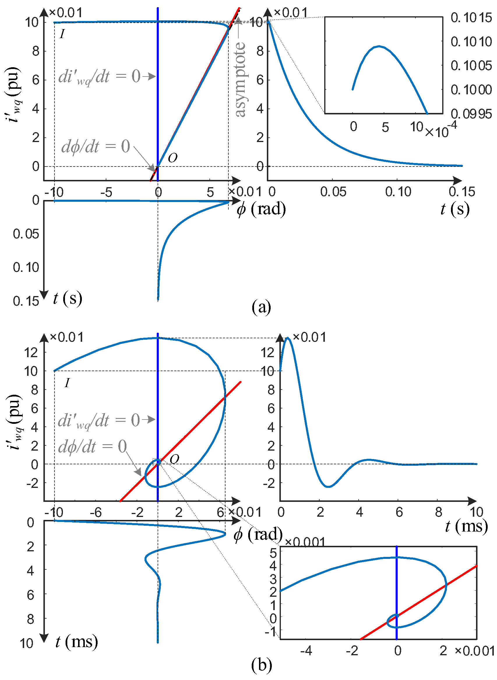
It should also be assumed that the initial point is I with the position (−0.1, 0.1), and the convergence process of the second-order simplified system is illustrated in Figure 9. From Figure 9a, it can be observed that the system converges along the asymptote, since the equilibrium point is a stable node. In Figure 9b, the equilibrium point become a stable focus due to a large ki3. Thus, although the convergence speed become large, there is an overshoot in the motion near the stable focus. Therefore, it can be concluded that a large ki3 can facilitate the system converge speed, causing both overshoot and oscillation. A trade-off should be considered to design an appropriate value for the control parameter ki3. Similar work can be made to further study the effects of other parameters on the system dynamic behaviors.
It is noteworthy that, when i′wq reaches the limitation i′wqmin or i′wqmax, the system state moves along the boundaries and it can still converge once the state reaches another section across the blue curve as long as the equilibrium point is in the allowable domain. In Equation (27), the range of i′wq is related to iwd, i.e., the active power Pw. While in Equation (24), the equilibrium point is related to the required reactive power Qw. The different equilibrium curves (or points) and domains under different Pw and Qw are depicted in Figure 10. In particular, the equilibrium point P1 (P1′) are beyond the domain, when both Pw and Qw are quite large, such as 1.0 and 0.9 (−0.9). The problem must be avoided in practice. To this end, a proper capacity of filters could be designed to result in a smaller Qw.
4.2. Stability Analysis of P-V Control
A simplified second-order equation of the HVDC subsystem can be obtained when the current transients are ignored.
According to Equations (28) and (29), when Pw increases, the voltage amplitude Ubm will increase, and thus the control loop Equation (28) will adjust the DC current reference. Once the firing angle regulated by the inner loop decreases, the actual DC current id will increase. According to Equation (29), Ubm will stop increasing and start to decrease, and finally the system will reach a new steady state.
4.3. Small-Signal Analysis and Parameters Design
Taking one of typical operating points, i.e., Pw = 0.8 pu and Qrc = 0.21 pu; as an example, the small-signal model of the overall system can be established in the RSEF, as shown in Figure 11. For the inner loop regulator, PI2 and PI4, of the WECS, the parameters can be set as kp2 (kp4) is 1.0, and ki2 (ki4) is 10, leading to a closed-loop bandwidth about 167 Hz. Moreover, typical parameters such as kp1 = 4.0, ki1 = 50 can be set for the outer loop active power regulator PI1, leading to a closed-loop bandwidth of about 20 Hz.
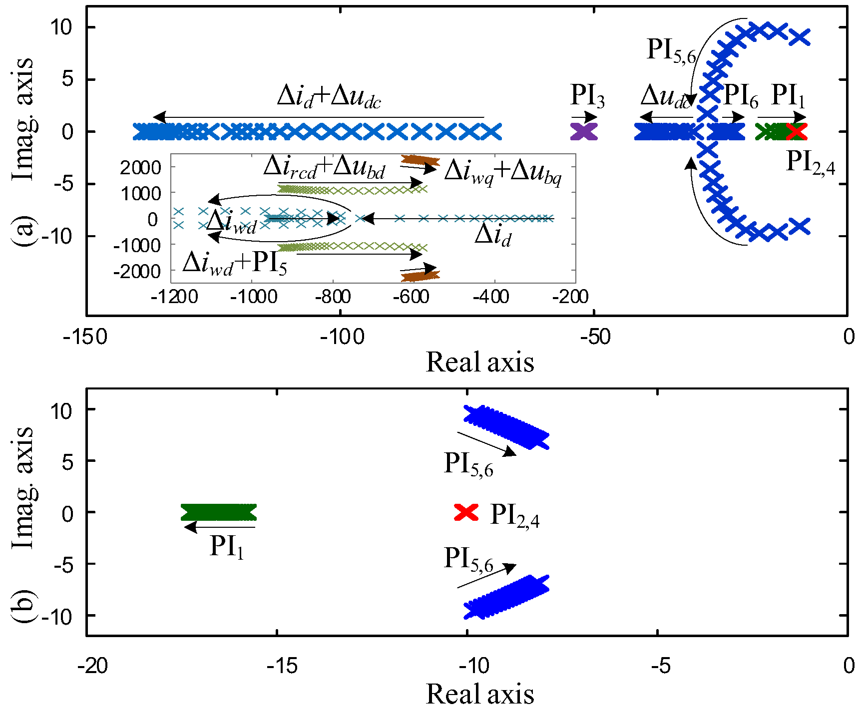
In particular, attention should be paid to the parameters of the developed outer loop reactive power control. As shown in Figure 12a, when ki3 becomes larger, the damping of PI3 increases. However, the loop will couple with the DC voltage when ki3 is too large, resulting in a pair of conjugate modes. It can be seen from Figure 12b that when kp3 increases, the damping of PI3 decreases, which thereafter leads to the coupling. However, the coupling disappears as kp3 continues to increase. Finally, kp3 ∈ [1.5, 2.0], and ki3 ∈ [20, 140] can be taken. Within the tuned parameter ranges, the closed-loop bandwidth is about 40 Hz.
A similar analysis can be performed to tune the parameters of the rectifier P-V controller. In Figure 13a, when ki5 becomes larger, the oscillation mode in PI5,6 disappears, but the damping of PI6 tends to decrease and the damping characteristics of both the voltage and current of the SEB are deteriorated. In Figure 13b, the larger kp5 is, the smaller the damping factor of PI5,6 is. Finally, kp5 ∈ [0.2, 0.5], ki5 ∈ [40, 100] can be selected. Note that typical parameters such as kp6 = 2.0 and ki6 = 20 are employed in the inner loop. Within the suggested parameter ranges, the outer and inner closed-loop bandwidths are approximately 5 Hz and 110 Hz respectively.
5. Simulation Results
Simulations are carried out on PSCAD/EMTDC to verify the proposed control scheme. The simulated system is shown in Figure 14, and the detailed parameters of the system are listed in Table 1. The employed monopole LCC-HVDC model is from the CIGRE benchmark model [33], both the rectifier and inverter of which are LCC-based. The rated capability of the system is 1000 MVA, and the reactive power capability of each set of AC 11/13 order harmonic filters is 50 MVar. The increase and decrease of the DC-side current of the WECS can simulate the changes of the input power of the back end.
5.1. System Startup
The WF is equivalent to a single WECS, and the system startup process is shown in Figure 15. Before the system startup, the capacitor of the WECS is charged by the configured battery, and thereafter the three-phase AC voltage of the SEB can be generated by the WECS at 0–0.3 s, as shown in Figure 15a. At 0.3 s, the DC-side current of the WECS starts to increase, and then the HVDC is unblocked, with the P-V control in the rectifier whereas the constant-voltage control in the inverter. Henceforth, the DC voltage of HVDC is generated gradually, as shown in Figure 15g. At 0.4 s, the battery configured at the DC bus of the WECS is withdrew, and the Q-f control in the WECS is switched on. Then, the active power continues increasing until to the rated point, as shown in Figure 15b,f. In Figure 15a, it can be observed that both the system frequency ω1 and the voltage of the SEB Ubm remain stable and are maintained at 1.0 pu in the final steady state. The active power generated from the WECS can be delivered into the receiving end grid through the LCC-HVDC transmission. The AC filters are connected to the SEB gradually when the reactive power from the WECS Qw is large than 0.1 pu (see Figure 15c), which can be regarded as the reactive power limit of the WECS. The reactive current iwq of the WECS is regulated automatically, so as to compensate the reactive power for the LCR under the condition that ubq = 0, as shown in Figure 15d,f. Moreover, Figure 15e indicates that the DC-side voltage of the WECS remains stable under the active power control of the WECS after the battery is withdrawn.
5.2. Operation under Disturbances
Under disturbances, such as fluctuations of active power and reactive power, the simulation results are shown in Figure 16, where the WF is equivalent to a single WECS with the PI-type Q-f control. In Figure 16, at 0.5 s, the DC-side current of the WECS starts to decrease, which simulates the decrease of the input active power from the front end of the WECS. Figure 16a shows that a small drop of the SEB voltage Ubm occurs. Then, the voltage returns to the rated value under the P-V control. At 2.0 s, the DC-side current rises to the original value, and a contrary phenomenon can be observed in Figure 16b. It should be noticed that the AC filters cannot be removed or added due to a time delay. Therefore, the reactive power difference between Qrc and Qfilter can be compensated by Qw. From 4 s to 9 s, several sets of filters are added and removed intentionally, in order to verify the performance of the Q-f control. From Figure 16d, it can be observed that the reactive current iwq automatically changes with the demand for reactive power under the condition that ubq = 0, guaranteeing the frequency stability. Accordingly, the reactive power differences between Qrc and Qfilter can be automatically compensated by the WECS, as shown in Figure 16c.
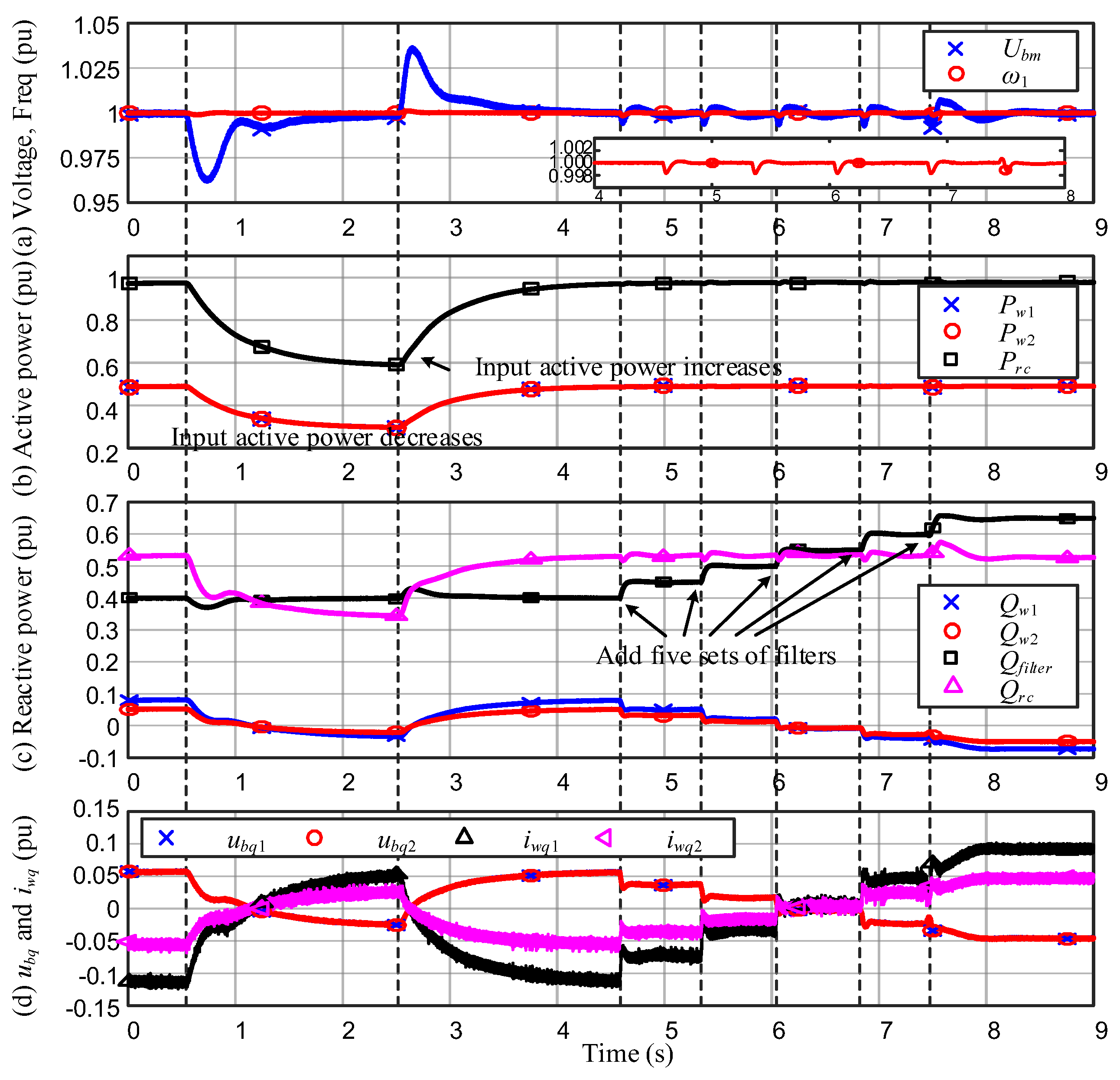
In order to evaluate the performance of the Q-f droop control in a multi-machine WF, the WF is represented by two WECSs with a P-type Q-f droop control. The capabilities of the two WECSs are the same (500 MVA) but the droop coefficients are different (2.0 versus 1.0). The simulation result is shown in Figure 17. The DC-side currents of the WECSs decrease at 0.5 s and then increase at 2.5 s. From 4.5 s to 7.5 s, several sets of AC filters are connected to the SEB gradually. The similar results compared with Figure 16 can be obtained. However, there is a small static error in ubq1,2 because of the adopted P-type droop control, as shown in Figure 17d. Moreover, from Figure 17d, it can be also observed that the shared reactive current by WECS1 iwq1 is twice that of WECS2 iwq2, due to the relationship between their droop coefficients.
It should be noted that the dynamic behaviors of the system is affected by both the system parameters and control parameters. The small-signal stability analysis performed in Section 4.3 just illustrates the results of one of the typical operating points. Similar repetitive work can be made to further study the effect of control parameters on the system stability at different operating points. Furthermore, as shown in Figure 9, the phase-plane analysis, together with time-domain state trajectory based on Equations (22) and (23), or Equations (28) and (29) can be employed to evaluate the effects of the system parameters and control parameters on the dynamic behaviors of the system in practical applications.
6. Conclusions
This paper proposed a novel coordinated control scheme for WFs with LCC-HVDC integration. The scheme comprises the Q-f control loop in the WECSs, and the P-V control loop in the LCR. The Q-f control maintains the system frequency and compensates for the reactive power for the LCR automatically, whereas the P-V control maintains the AC bus voltage and realizes the active power balance of the sending-end bus of the HVDC. Thus, the scheme addresses both the voltage and frequency stability, based on the coordination between the WF and the LCR.
The distinguishing features of the scheme can be concluded as follows: (1) there are no commonly used PLLs in the controllers of WECSs, and consequently, the frequency and synchronization stability issues introduced by PLLs can be avoided; (2) the reactive power droop instead of the active power droop is adopted while being applied to achieve synchronization control and reactive power sharing in multi-machine systems, and therefore, the maximum power point tracking of WFs remains unaffected; (3) the scheme can be utilized in more universal scenarios, as long as the core topology is the VSI with LCR connection, such as WFs and photovoltaic power plants with LCC-based rectifier HVDC integration. Our future work will focus on the control and protection algorithms during fault operation, e.g., voltage-dependent current order limits (VDCOLs) for LCC-HVDC and low voltage ride-through (LVRT) for WECS.
Author Contributions
Conceptualization, X.H. and H.G.; Methodology, X.H.; Validation, X.H, H.G. and G.Y.; Writing—Original Draft Preparation, X.H.; Writing—Review & Editing, H.G., G.Y. and X.Z.; Supervision, H.G. and X.Z.; Project Administration, G.Y.
Funding
This work was supported by the National Natural Science Foundation of China (Nos. 61722307, U1510208, and 51711530235).
Conflicts of Interest
The authors declare no conflict of interest.
References
- Mendoza-Vizcaino, J.; Sumper, A.; Galceran-Arellano, S. PV, Wind and storage integration on small islands for the fulfilment of the 50-50 renewable electricity generation target. Sustainability 2017, 9, 905. [Google Scholar] [CrossRef]
- Korkas, C.D.; Baldi, S.; Michailidis, I.; Kosmatopoulos, E.B. Occupancy-based demand response and thermal comfort optimization in microgrids with renewable energy sources and energy storage. Appl. Energy 2016, 163, 93–104. [Google Scholar] [CrossRef] [Green Version]
- Tavakoli, M.; Shokridehakia, F.; Marzband, M.; Godina, R.; Pouresmaeil, E. A two stage hierarchical control approach for the optimal energy management in commercial building microgrids based on local wind power and PEVs. Sustain. Cities Soc. 2018, 41, 332–340. [Google Scholar] [CrossRef]
- Zhou, H.; Yang, G.; Wang, J. Modeling, analysis, and control for the rectifier of hybrid HVdc systems for DFIG-based wind farms. IEEE Trans. Energy Convers. 2011, 26, 340–353. [Google Scholar] [CrossRef]
- Brenna, M.; Foiadelli, F.; Longo, M.; Zaninelli, D. Improvement of wind energy production through HVDC systems. Energies 2017, 10, 157. [Google Scholar] [CrossRef]
- Smailes, M.; Ng, C.; Mckeever, P.; Shek, J.; Theotokatos, G.; Abusara, M. Hybrid, multi-megawatt HVDC transformer topology comparison for future offshore wind farms. Energies 2017, 10, 851. [Google Scholar] [CrossRef]
- Halawa, E.; James, G.; Shi, X.R.; Sari, N.H.; Nepal, R. The prospect for an Australian-Asian power grid: A critical appraisal. Energies 2018, 11, 200. [Google Scholar] [CrossRef]
- Pena, R.; Clare, J.C.; Asher, G.M. Doubly fed induction generator using back-to-back PWM converters and its application to variable-speed wind-energy generation. IEE Proc. Electr. Power Appl. 1996, 143, 231–241. [Google Scholar] [CrossRef]
- Ma, S.; Geng, H.; Liu, L.; Yang, G.; Pal, B.C. Grid-Synchronization stability improvement of large scale wind farm during severe grid fault. IEEE Trans. Power Syst. 2018, 33, 216–226. [Google Scholar] [CrossRef]
- Zhou, H.; Yang, G.; Wang, J.; Geng, H. Control of a hybrid high-voltage DC connection for large doubly fed induction generator-based wind farms. IET Renew. Power Gener. 2011, 5, 36–47. [Google Scholar] [CrossRef]
- Zhou, H.; Yang, G.; Geng, H. Grid integration of DFIG-based offshore wind farms with hybrid HVDC connection. In Proceedings of the 2008 International Conference on Electrical Machines and Systems, Wuhan, China, 17–20 October 2008. [Google Scholar]
- Bozhko, S.V.; Blasco-Gimnez, R.; Li, R.; Clare, J.C.; Asher, G.M. Control of offshore DFIG-based wind farm grid with line-commutated HVDC connection. IEEE Trans. Energy Convers. 2007, 22, 71–78. [Google Scholar] [CrossRef]
- Bozhko, S.V.; Asher, G.; Li, R.; Clare, J.; Yao, L. Large offshore DFIG-based wind farm with line-commutated HVDC connection to the main grid: Engineering studies. IEEE Trans. Energy Convers. 2008, 23, 119–127. [Google Scholar] [CrossRef]
- Xiang, D.; Ran, L.; Bumby, J.R.; Tavner, P.J.; Yang, S. Coordinated control of an HVDC link and doubly fed induction generators in a large offshore wind farm. IEEE Trans. Power Deliv. 2006, 21, 463–471. [Google Scholar] [CrossRef]
- Li, R.; Bozhko, S.; Asher, G. Frequency control design for offshore wind farm grid with LCC-HVDC link connection. IEEE Trans. Power Electron. 2008, 23, 1085–1092. [Google Scholar] [CrossRef]
- Zhang, M.; Yuan, X.; Hu, J.; Wang, S.; Ma, S.; He, Q.; Yi, J. Wind power transmission through LCC-HVDC with wind turbine inertial and primary frequency supports. In Proceedings of the 2015 IEEE Power & Energy Society General Meeting, Denver, CO, USA, 26–30 July 2015. [Google Scholar]
- Cardiel-Álvarez, M.Á.; Rodriguez-Amenedo, J.L.; Arnaltes, S.; Montilla-DJesus, M.E. Modeling and control of LCC rectifiers for offshore wind farms connected by HVDC links. IEEE Trans. Energy Convers. 2017, 32, 1284–1296. [Google Scholar] [CrossRef]
- Yin, H.; Fan, L.; Miao, Z. Coordination between DFIG-based wind farm and LCC-HVDC transmission considering limiting factors. In Proceedings of the IEEE 2011 EnergyTech, Cleveland, OH, USA, 25–26 May 2011. [Google Scholar]
- Yin, H.; Fan, L. Modeling and control of DFIG-based large offshore wind farm with HVDC-link integration. In Proceedings of the 41st North American Power Symposium, Starkville, MS, USA, 4–6 October 2009. [Google Scholar]
- Blasco-Gimenez, R.; Añó-Villalba, S.; Rodríguez-D’Derlée, J.; Morant, F.; Bernal-Perez, S. Distributed voltage and frequency control of offshore wind farms connected with a diode-based HVdc link. IEEE Trans. Power Electron. 2010, 25, 3095–3105. [Google Scholar] [CrossRef]
- Yu, L.; Li, R.; Xu, L. Distributed PLL-based control of offshore wind turbine connected with diode-rectifier based HVDC systems. IEEE Trans. Power Deliv. 2018, 33, 1328–1336. [Google Scholar] [CrossRef]
- Cardiel-Álvarez, M.Á.; Arnaltes, S.; Rodriguez-Amenedo, J.L.; Nami, A. Decentralized control of offshore wind farms connected to diode-based HVDC links. IEEE Trans. Energy Convers. 2018, 33, 1233–1241. [Google Scholar] [CrossRef]
- Xi, X.; Geng, H.; Yang, G. Enhanced model of the doubly fed induction generator-based wind farm for small-signal stability studies of weak power system. IET Renew. Power Gener. 2014, 8, 765–774. [Google Scholar] [CrossRef]
- Zhang, Y.; Ooi, B.T. Stand-Alone doubly-fed induction generators (DFIGs) with autonomous frequency control. IEEE Trans. Power Deliv. 2013, 28, 752–760. [Google Scholar] [CrossRef]
- Pena, R.; Clare, J.C.; Asher, G.M. A doubly fed induction generator using back-to-back PWM converters supplying an isolated load from a variable speed wind turbine. IEE Proc. Electr. Power Appl. 1996, 143, 380–387. [Google Scholar] [CrossRef]
- Abdoune, F.; Aouzellag, D.; Ghedamsi, K. Terminal voltage build-up and control of a DFIG based stand-alone wind energy conversion system. Renew. Energy 2016, 97, 468–480. [Google Scholar] [CrossRef]
- Li, D.; Shen, Q.; Liu, Z.; Wang, H.; Ding, M.; Liu, F. Auto-disturbance rejection control for the stator voltage in a stand-alone DFIG-based wind energy conversion system. In Proceedings of the 2016 35th Chinese Control Conference (CCC), Chengdu, China, 27–29 July 2016. [Google Scholar]
- Fazeli, M.; Asher, G.; Klumpner, C.; Yao, L. Novel integration of DFIG-based wind generators within microgrids. IEEE Trans. Energy Convers. 2011, 26, 840–850. [Google Scholar] [CrossRef]
- Fazeli, M.; Bozhko, S.V.; Asher, G.M.; Yao, L. Voltage and frequency control of offshore DFIG-based wind farms with line commutated HVDC connection. In Proceedings of the 2008 4th IET Conference on Power Electronics, Machines and Drives, York, UK, 2–4 April 2008. [Google Scholar]
- Huang, L.; Xin, H.; Zhang, L.; Wang, Z.; Wu, K.; Wang, H. Synchronization and frequency regulation of DFIG-based wind turbine generators with synchronized control. IEEE Trans. Energy Convers. 2017, 32, 1251–1262. [Google Scholar] [CrossRef]
- Zhong, Q.-C.; Nguyen, P.-L.; Ma, Z.; Sheng, W. Self-synchronized synchronverters: Inverters without a dedicated synchronization unit. IEEE Trans. Power Electron. 2014, 29, 617–630. [Google Scholar] [CrossRef]
- Kalman, R.E. Phase-plane analysis of automatic control systems with nonlinear gain elements. Trans. AIEE 1955, 73, 383–390. [Google Scholar] [CrossRef]
- Atighechi, H.; Chiniforoosh, S.; Jatskevich, J.; Davoudi, A.; Martinez, J.A.; Faruque, M.O.; Sood, V.; Saeedifard, M.; Cano, J.M.; Mahseredjian, J.; et al. Dynamic average-value modeling of CIGRE HVDC benchmark system. IEEE Trans. Power Deliv. 2014, 29, 2046–2054. [Google Scholar] [CrossRef]
Figure 1.
System topology.

Figure 2.
Equivalent circuit, where the wind farm (WF) is represented by a single wind energy conversion systems (WECS) just for a simplified system model. Note that the proposed control scheme is applicable for multiple WECSs (see the next section for more details).
Figure 2.
Equivalent circuit, where the wind farm (WF) is represented by a single wind energy conversion systems (WECS) just for a simplified system model. Note that the proposed control scheme is applicable for multiple WECSs (see the next section for more details).

Figure 3.
(a) Conventional vector control (VC) versus (b) proposed reactive power-based frequency (Q-f) control for voltage source inverters (VSIs) of WECSs. In actual practice, the controlled variable ubq can be replaced by the local voltage information instead of sending-end bus (SEB) voltage information. Since the critical information is the voltage-phase angle rather than the voltage amplitude, the spatial distribution feature of the voltage amplitude has litter influences on the Q-f control performance.
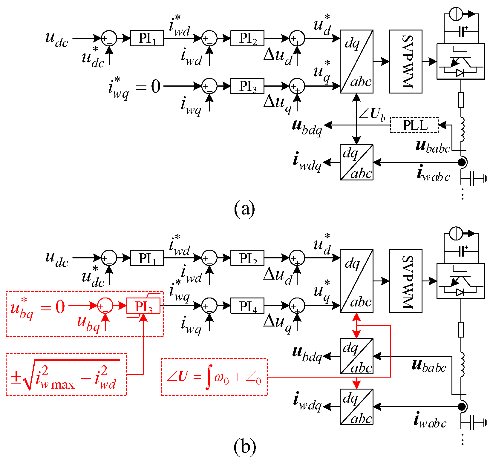
Figure 4.
Vector diagrams in the rated synchronous reference frame (RSRF) under different control algorithms: (a) Conventional VC with iwq = 0; (b) Self-oriented control with iwq = 0; (c) Proposed Q-f control with ubq = 0.
Figure 4.
Vector diagrams in the rated synchronous reference frame (RSRF) under different control algorithms: (a) Conventional VC with iwq = 0; (b) Self-oriented control with iwq = 0; (c) Proposed Q-f control with ubq = 0.
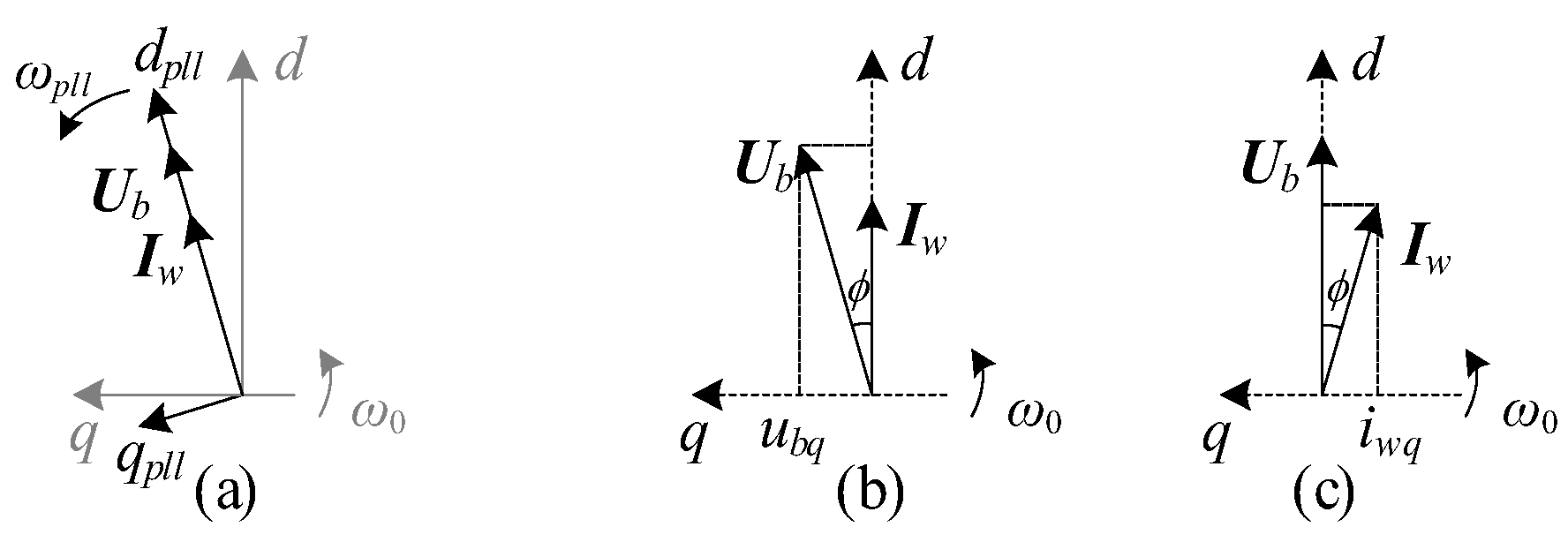
Figure 5.
Reactive current and reactive power sharing relationship with the P-type droop control. (a) Reactive current sharing relationship; (b) reactive power sharing relationship.
Figure 5.
Reactive current and reactive power sharing relationship with the P-type droop control. (a) Reactive current sharing relationship; (b) reactive power sharing relationship.

Figure 6.
Vector diagrams under the condition that Ub remains constant. (a) A smaller active current iwd (or Pw); (b) a larger active current iwd.
Figure 6.
Vector diagrams under the condition that Ub remains constant. (a) A smaller active current iwd (or Pw); (b) a larger active current iwd.

Figure 7.
Proposed power based voltage (P-V) control for LCR.
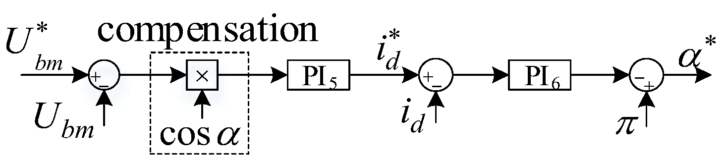
Figure 8.
Phase plane ϕ − i′wq with the Q-f control.
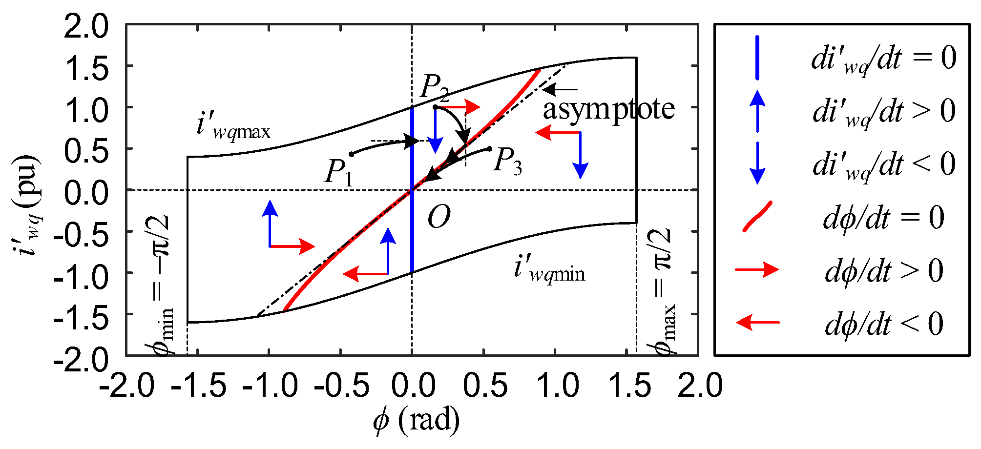
Figure 9.
Convergence process of the second-order simplified system composed of Equations (22) and (23), from the initial point I. (a) kp3 = 0.6, ki3 = 50; (b) kp3 = 0.3, ki3 = 2000.
Figure 9.
Convergence process of the second-order simplified system composed of Equations (22) and (23), from the initial point I. (a) kp3 = 0.6, ki3 = 50; (b) kp3 = 0.3, ki3 = 2000.

Figure 10.
Different equilibrium curves and domains under different Pw and Qw.
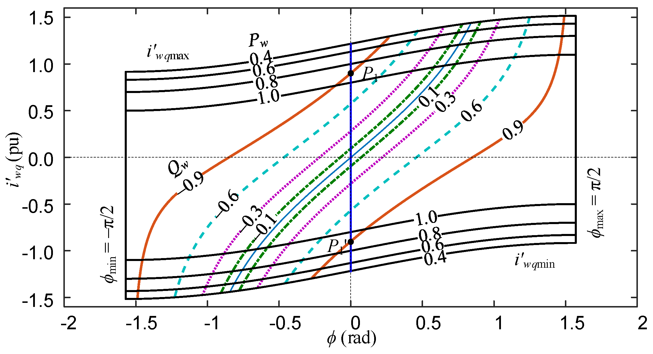
Figure 11.
Small-signal model of the system.
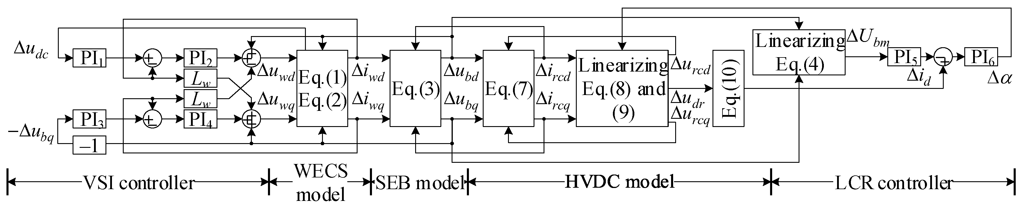
Figure 12.
Root loci of the small-signal model. (a) kp3 = 1.3 and ki3 changes from 50 to 140; (b) ki3 = 130 and kp3 changes from 0.3 to 2.0.
Figure 12.
Root loci of the small-signal model. (a) kp3 = 1.3 and ki3 changes from 50 to 140; (b) ki3 = 130 and kp3 changes from 0.3 to 2.0.
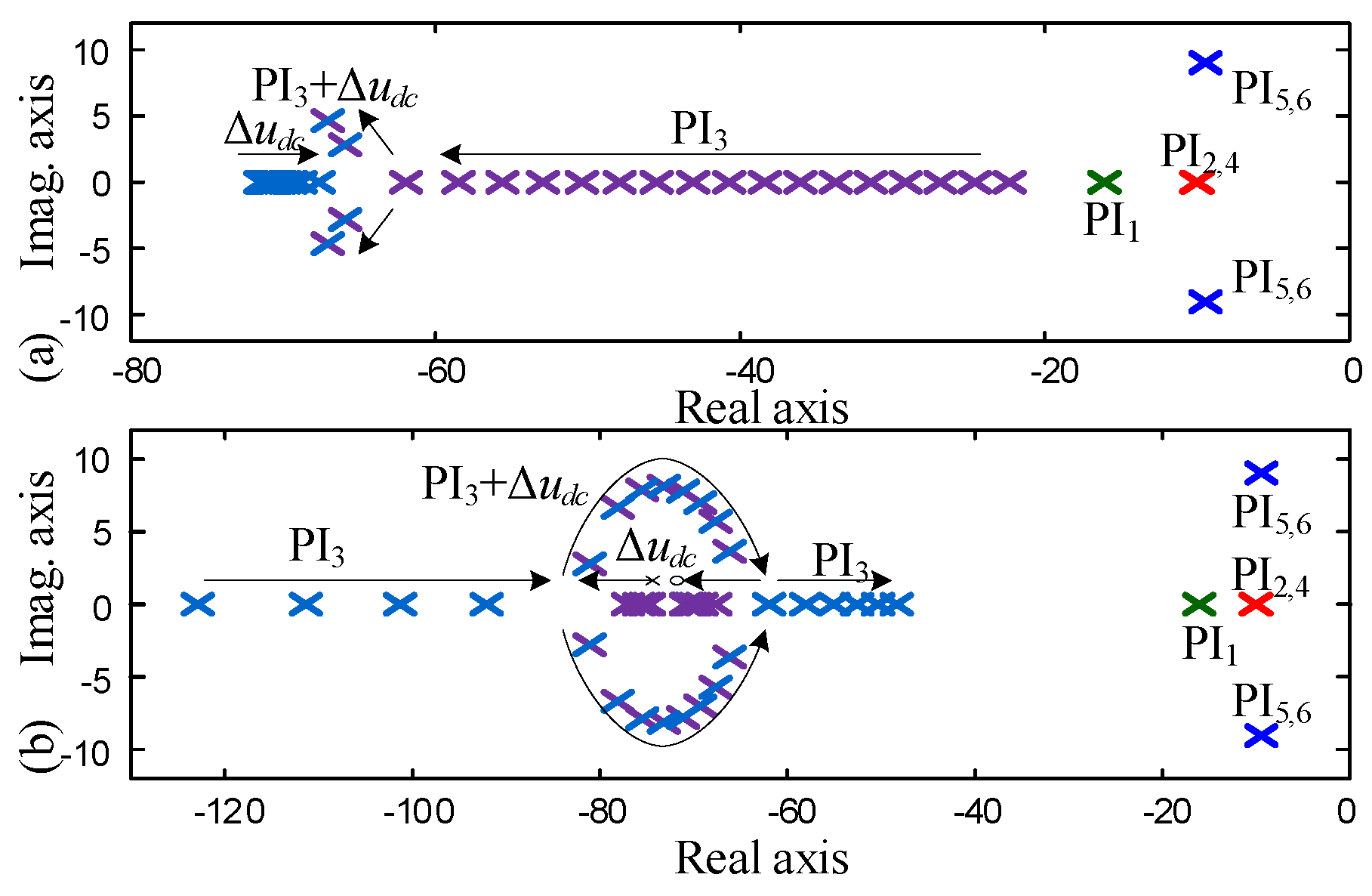
Figure 13.
Root loci of the small-signal model. (a) kp5 = 0.4 and ki5 changes from 50 to 1000; (b) ki5 = 50 and kp5 changes from 0.1 to 2.0.
Figure 13.
Root loci of the small-signal model. (a) kp5 = 0.4 and ki5 changes from 50 to 1000; (b) ki5 = 50 and kp5 changes from 0.1 to 2.0.

Figure 14.
Simulated system.

Figure 15.
Simulation result of the system startup. (a) Sending-end bus voltage and frequency; (b) active power; (c) reactive power; (d) dq-axis sending-end bus voltage; (e) WECS DC-link voltage; (f) WECS output current; (g) HVDC DC-link voltage and current.
Figure 15.
Simulation result of the system startup. (a) Sending-end bus voltage and frequency; (b) active power; (c) reactive power; (d) dq-axis sending-end bus voltage; (e) WECS DC-link voltage; (f) WECS output current; (g) HVDC DC-link voltage and current.
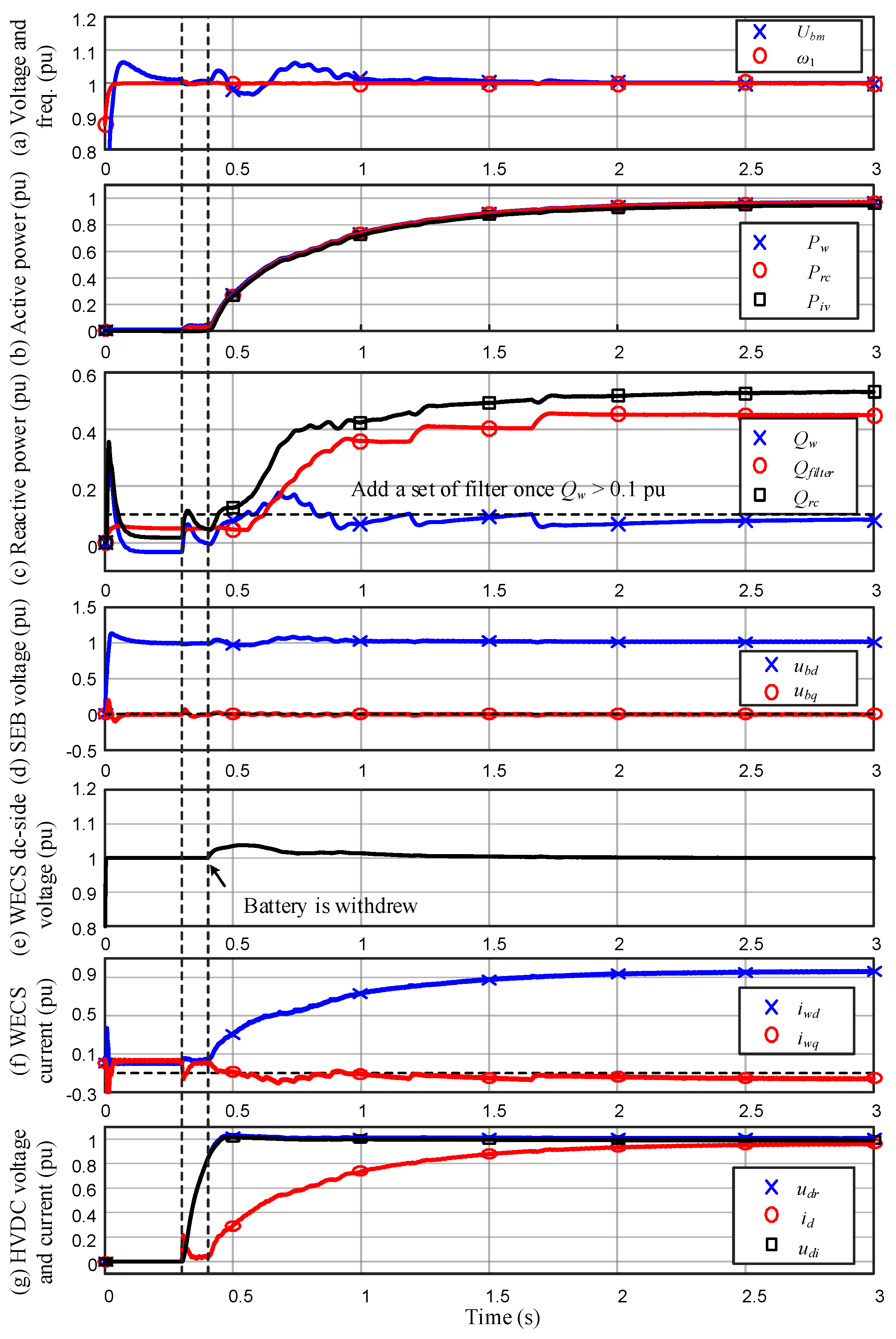
Figure 16.
Simulation results under external disturbances, where the WF is represented by a single WECS with the PI-type Q-f control. (a) Sending-end bus voltage and frequency; (b) active power; (c) reactive power; (d) dq-axis sending-end bus voltage.
Figure 16.
Simulation results under external disturbances, where the WF is represented by a single WECS with the PI-type Q-f control. (a) Sending-end bus voltage and frequency; (b) active power; (c) reactive power; (d) dq-axis sending-end bus voltage.
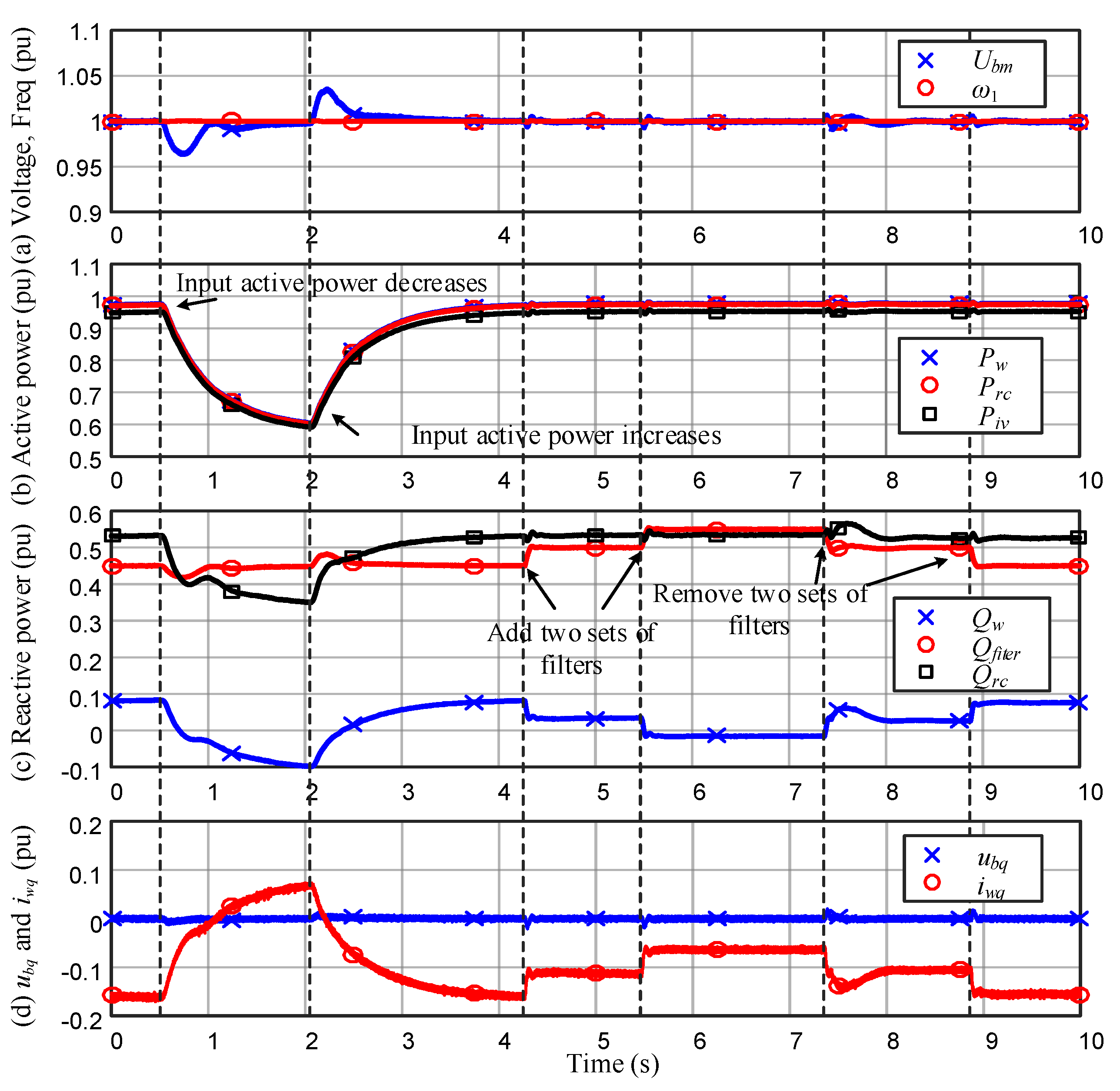
Figure 17.
Simulation results under external disturbances, where the WF is represented by two WECSs with the P-type Q-f droop control. (a) Sending-end bus voltage and frequency; (b) active power; (c) reactive power; (d) dq-axis sending-end bus voltage. Note that Pw1, Pw2 denote the active powers outputted by both the WECSs, respectively, similar for Qw1, Qw2. Qfilter denotes the reactive power generated by the filters.

Table 1.
Parameters of the simulated system.
| Wind Energy Conversion System | Cdc | 90,000 uF for 1.5 MVA capacity |
| Rw | 0.001 pu | |
| Lw | 0.3 pu | |
| Sending-End Bus | Cf | 0.05 pu for each set of filter |
| High Voltage Direct Current System | Rrc | 0.001 pu |
| Lrc | 0.18 pu | |
| Ld | 1.1936 H | |
| Rd | 5 Ω |
© 2018 by the authors. Licensee MDPI, Basel, Switzerland. This article is an open access article distributed under the terms and conditions of the Creative Commons Attribution (CC BY) license (http://creativecommons.org/licenses/by/4.0/).
Share and Cite
MDPI and ACS Style
He, X.; Geng, H.; Yang, G.; Zou, X. Coordinated Control for Large-Scale Wind Farms with LCC-HVDC Integration. Energies 2018, 11, 2207. https://doi.org/10.3390/en11092207
AMA Style
He X, Geng H, Yang G, Zou X. Coordinated Control for Large-Scale Wind Farms with LCC-HVDC Integration. Energies. 2018; 11(9):2207. https://doi.org/10.3390/en11092207
Chicago/Turabian StyleHe, Xiuqiang, Hua Geng, Geng Yang, and Xin Zou. 2018. "Coordinated Control for Large-Scale Wind Farms with LCC-HVDC Integration" Energies 11, no. 9: 2207. https://doi.org/10.3390/en11092207
Note that from the first issue of 2016, this journal uses article numbers instead of page numbers. See further details here.