Combinatory Finite Element and Artificial Neural Network Model for Predicting Performance of Thermoelectric Generator


1
Center for Energy Harvesting Materials and Systems (CEHMS), Virginia Tech, Blacksburg, VA 24061, USA
2
Department of Mechanical Engineering, Virginia Tech, Blacksburg, VA 24061, USA
3
Institute for Critical Technology and Applied Science (ICTAS), 325 Stanger Street, Blacksburg, VA 24061, USA
4
Materials Research Institute, Penn State, University Park, PA 16802, USA
*
Author to whom correspondence should be addressed.
Energies 2018, 11(9), 2216; https://doi.org/10.3390/en11092216
Submission received: 2 August 2018
/
Revised: 17 August 2018
/
Accepted: 17 August 2018
/
Published: 24 August 2018
Abstract
:Thermoelectric generators (TEGs) are rapidly becoming the mainstream technology for converting thermal energy into electrical energy. The rise in the continuous deployment of TEGs is related to advancements in materials, figure of merit, and methods for module manufacturing. However, rapid optimization techniques for TEGs have not kept pace with these advancements, which presents a challenge regarding tailoring the device architecture for varying operating conditions. Here, we address this challenge by providing artificial neural network (ANN) models that can predict TEG performance on demand. Out of the several ANN models considered for TEGs, the most efficient one consists of two hidden layers with six neurons in each layer. The model predicted TEG power with an accuracy of ±0.1 W, and TEG efficiency with an accuracy of ±0.2%. The trained ANN model required only 26.4 ms per data point for predicting TEG performance against the 6.0 minutes needed for the traditional numerical simulations.
1. Introduction
A thermoelectric generator (TEG) module consists of multiple thermocouples, which are connected electrically in a series and thermally in parallel. When a thermal gradient is applied across the two ends of a TEG module, electrons in the n-type legs and holes in the p-type legs move from the hot side to the cold side, resulting in the flow of electrical current [1]. In other words, a TEG is a solid-state heat engine that directly converts heat into electricity with no moving parts or harmful discharge [2]. The principle for energy conversion is based on a thermoelectric effect that includes three different thermal-to-electric phenomena: the Seebeck effect, the Peltier effect, and the Thomson effect [3]. The Seebeck effect results in an induced voltage in response to the temperature difference applied across the two ends of a thermocouple, where the induced voltage is directly proportional to the temperature difference [4,5]. The Peltier effect is the reverse of the Seebeck effect, and it results in cooling or heating at the two junctions of a thermocouple when an electric current passes through it [6]. The Peltier heat is directly proportional to the electric current, but its sign (cooling or heating) depends upon the direction of the electric current. Both the Seebeck and Peltier effects require a thermocouple, which consists of two dissimilar materials. However, the Thomson effect occurs in a single material when it is non-uniformly heated and an electric current is passed through it. Continuous Seebeck and Peltier effects due to the combined effect of a spatial temperature gradient and an electric current result in the Thomson heat, which is proportional to the electric current and absorbed or released based on the direction of the current [4].
Continuous efforts have been made toward developing high performance n-type and p-type thermoelectric (TE) materials [1,7,8,9]. The performance of TE materials is measured in terms of a dimensionless metric called the figure of merit, which is denoted as ZT. It combines three key material properties: thermal conductivity (κ), electrical resistivity (), and the Seebeck coefficient (S), along with the absolute temperature (T), and it is given as [10,11]. The magnitude of ZT for most of the commercial thermoelectric materials is close to unity; however, recent studies have reported higher values for some of the state-of-the-art TE materials, such as a quantum-dot superlattice with ZT ~ 3.5 at 575 K [12], a superlattice structure with ZT ~ 2.4 at 300 K and ZT ~ 2.9 at 400 K [13], and lead antimony silver telluride with ZT ~ 2.2 at 800 K [14]. The thermoelectric modules built using nanostructured materials have been reported to exhibit thermal-to-electrical energy conversion efficiency up to 10% at a temperature difference of 500 K [15].
The performance of TEG modules depends not only on the ZT of the TE material, but also on the geometric dimensions of the thermocouples and operating conditions such as the temperature difference and electrical load [16,17]. Several researchers in the past have attempted to optimize p–n leg geometry comprising of length, a cross-sectional area, and the number of thermocouples [18,19,20,21]. A few studies have attempted to provide optimal shape factor parameters such as the area ratio for p–n legs (Ap/An), the aspect ratio (leg length/leg area), and the slenderness ratio ((Ap/Lp)/(An/Ln), where Ap and An denote base area and Lp and Ln denote length of p- and n-type legs) [22,23]. However, these parameter changes depend upon the TE material used for fabricating TEG legs, the materials used in assembling the TEG modules, and operating conditions. Experimental studies are often expensive and time-consuming when used to optimize all of the variables. Therefore, analytical and numerical models have been developed using simplified one-dimensional models [24,25] as well as complex three-dimensional models [5,26,27].
Thermoelectric generators are now being utilized for a variety of applications, such as power sources for wireless sensor nodes in satellites, space probes, and unmanned remote facilities [28,29]. TEGs are being developed for use in automobiles for generating electricity from exhaust gases in order to improve overall engine efficiency [30]. Several studies have testified TEGs as a viable option for waste heat recovery in domestic, industrial, and other processes [2,31,32,33]. Recently, TEGs have been introduced in the consumer market as a power device to charge small electronics such as sensors and cell phones by utilizing heat from candles [34] and propane stoves [35]. Duran et al. have discussed thermoelectric power plants and proposed the lean maintenance philosophy to improve maintenance efficiency [36]. It has been suggested that the use of TEGs to power the different elements of the smart grid could provide considerable advantages for system suppliers and power companies by dramatically reducing the need to replace the batteries in wireless sensor networks, and thereby saving substantial operating costs [37]. Going forward, as TEGs become mainstream technology, the reliance on a predictive simulation model will continue to increase. Thus, there is a necessity to provide fast and reliable models that can provide on-demand module optimization. Materials behavior-based thermoelectric differential equations are quite difficult to be utilized for on-demand module optimization, as they require a considerable amount of computational power and time. The complexity further increases when the temperature-dependent nature of thermoelectric material properties, such as their thermal conductivity, electrical resistivity, and Seebeck coefficient, and the contribution due to contact resistances and environmental effects are included in the study. The thermoelectric consecutive expressions require numerical techniques and commercial finite element codes to find the numerical solutions. These codes may not be readily available. These difficulties limit the utility of computational studies, especially in a manufacturing environment where real-time decisions need to be made in order to control the design process [38]. In this scenario, artificial neural network (ANN) models can provide an effective real-time solution that is compatible with the manufacturing process environment [39].
An artificial neural network is analogous to the complex computing environment of interconnected neurons in a human brain. Similar to the human brain, a given ANN model is first trained using an available database for a given process application. Once the ANN model has been trained, it can simulate the outcome of that process in real-time, facilitating real-time decisions [40,41]. A few attempts have been made in the literature to develop traditional ANN models for predicting TEG output [42,43,44]. Here, we provide a hybrid physico-neural network model that can predict TEG performance with a high degree of accuracy. The model is implemented in two steps: first, we solve the physical equations of thermoelectricity for power and efficiency for a given range of geometric parameters and resistive loads using the finite element method. The resulting power and efficiency data are used to train ANN models. Second, the ANN model is utilized to evaluate the effect of the leg cross-sectional area, leg length, and resistive load on TEG performance. Out of several ANN models considered, the most efficient ANN model was determined to be one with two hidden layers, each having six neurons. This model was able to predict power with an accuracy of ±0.1 W, and efficiency with an accuracy ±0.2%.
2. Models and Methods
2.1. Thermoelectric Model
The open circuit voltage () across the two terminals of a TEG thermocouple can be analytically obtained using a one-dimensional model by integrating the Seebeck coefficients (α) over the given temperature difference.
where and denote the temperature-dependent Seebeck coefficient of the p-type and n-type legs, and and denote the hot side and cold side temperatures. In order to simplify the calculation, it is convenient to calculate the average Seebeck coefficients, and , which are given as:
Therefore, the Seebeck coefficient, α, of a thermocouple can be simply expressed as:
Considering a TEG module consisting of N thermocouples, the open circuit voltage across the two terminals of the module can be calculated as [3]:
The rate of thermal energy absorbed on the hot side, , and released on the cold side, , of the TEG module operating in a steady-state condition is expressed as [45,46]:
where denotes the internal electrical resistance and denotes the internal thermal conductance of the individual thermocouple. The output power of the TEG module can be calculated using:
where the current, I, in the TEG module connected to an external resistive load, R, is given as:
The thermal-to-electrical energy conversion efficiency of the TEG module can be obtained as:
Using Equations (8)–(10), the maximum thermal-to-electrical energy conversion efficiency of an ideal TEG with no contact resistances or thermal losses can be determined as [47]:
where and .
The one-dimensional model provides reasonable results when the thermal gradient is small, material properties can be taken as constant with temperature, and contact resistances are negligible. However, in practice, the assumption of one-dimensionality fails as the thermal gradient is increased and the environmental effects, such as the convective or radiative thermal losses, need to be taken into consideration. A robust three-dimensional model is needed to solve the coupled thermoelectric equations, which are given as [48,49]:
where , and . stand for the heat flux vector, current density vector, and electric field intensity vector, respectively, α and π are the Seebeck and Peltier coefficients, and σ and κ are the electrical and thermal conductivity of the TE material.
2.2. Finite Element Analysis
The thermoelectric equations given by Equations (12) and (13) are coupled. In order to numerically model a TEG, we require the governing equations in the discretized form with the appropriate boundary conditions. In this study, we have used a commercial finite element analysis (FEA) code, ANSYS v17.0 (Release 17.0, ANSYS, Inc., 275 Technology Drive, Canonsburg, PA, USA), which deduces the thermoelectric constitutive equations in the form of a finite element matrix equation of thermoelectricity as [50]:
where and are the finite element specific heat matrix and dielectric permittivity coefficient matrix, respectively; , , and are the finite element thermal conductivity matrix, electrical conductivity coefficient matrix, and Seebeck coefficient coupling matrix, respectively; denotes the sum of the finite element heat generation load and convection surface heat flow vectors; is the finite element Peltier heat load vector; and , , and are vectors of the finite element nodal temperature, nodal electric potential, and nodal current, respectively.
Due to the nonlinearity of the governing equations, the full Newton–Raphson scheme was deployed to obtain the finite element solution. The hot side and the cold side of the TEG module were assigned constant temperature thermal boundary conditions and the heat losses along the side surfaces of the p–n legs were ignored. We have considered a constant electrical contact resistance of 1.0 × 10⁻⁹ Ω-m2 and a thermal contact conductance of 2.2 × 10⁻⁴ m2KW−1, which are well within the range for the contact resistances reported in the literature [51,52,53,54]. We employed SOLID226 (a 3D 20-node hexahedron/brick) elements to discretize the FEA model. The mesh independency test was also performed to ensure that the numerical results are independent of the grid sizes. Lastly, in order to validate the finite element model, the numerical results were compared against the experimental results provided in Hao et al. [55]. Figure 1a,b depicts the comparison between the experimental and numerical results. The differences between the numerical results (with contact resistances) and experimental results for the output power and efficiency were found to be 1.6% and 2.1%, respectively, at 513 K.
2.3. Artificial Neural Network (ANN) Model
As mentioned in Section 1, an ANN model is inspired by the biological neural networks in human brains [56]. Broadly, it consists of an input layer, which contains one or more independent variables, an output layer, which contains the dependent variables, and one or several hidden layers in between, which contain numerous nodes or cells connected in complex patterns to permit for a variety of interconnections among the input variables to obtain the desired output [38]. In this study, there are three input variables: leg length, leg cross-sectional area, and resistive load. There are two output variables: power and efficiency. In order to achieve input-to-output mapping, we employed a multi-layer feedforward neural network architecture, where the information flows only in a forward direction, from the input to the output nodes through the hidden nodes. Mathematically, the input–output relation in a multi-layer feedforward neural network is expressed as [57]:
where denotes the output vector in the kth layer, and W and B represent connection and bias weight matrices, respectively. F is an activation function, and we have considered it as a sigmoid function, which is given as [38]:
Theoretically, one hidden layer with an adequate number of neurons is sufficient to produce excellent results; however, in practice, more hidden layers are needed to achieve expected results. There is no fixed rule to determine the adequate number of neurons in the hidden layer. Typically, increasing the number of neurons increases the power of the network, but it also increases the computational expense. In addition, an excessively large number of neurons increases the likelihood to produce overfitting [58]. In this study, we have followed the method of a simple-to-complex approach in which we start with a minimum number of neurons, and keep on adding an additional neuron until adding one does not improve the training accuracy. We have considered two hidden layers, and the number of neurons in each hidden layer was varied between one and 10 in order to determine the optimum value. The Levenberg–Marquardt algorithm was employed for network training. The Levenberg–Marquardt algorithm, which is also called the damped least-squares method, is a very popular training technique that is used in ANN because it is an interpolation between the Gauss–Newton method and the gradient descent method. Mathematically, it is expressed as [59]:
where i is the number of iteration steps, J is the Jacobian matrix that contains first derivatives of the network errors with respect to the weights and biases, and e is a vector of network errors. The scalar µ is varied between zero and a large number. A value of μ = 0 indicates Newton’s method, and when µ is large, it becomes a gradient descent method with a small step size [59].
In order to achieve good generalization, we employed a method of early stopping [60]. Such a method has been used in prior studies [61,62,63], and it has been found to be very effective. In this technique, the available input dataset is divided into three subsets: training set, validation set, and test set. As the training progresses, ideally, the error on the test set as well as the validation set should decrease. In case the network begins to overfit, the validation error begins to rise. If the rise in validation error continues for a fixed number of iterations, the training is stopped and the weights and biases at the minimum validation error are returned [60]. The error function that is typically used to monitor the performance of feedforward neural networks is the mean sum of squares of the network errors, which is given as:
where is the error term in the ith iteration and N is the total number of data points in a given subset. Sometimes, it is convenient to express the ANN error as the root mean square error (RMSE), which is given as:
In this study, there are three input parameters and we have considered five levels for each one of them for performing the parametric study. Therefore, our dataset consisted of 53 = 125 data points. We have divided input data randomly such that the first 60% of the samples are allotted to the training set, the next 20% of the samples are assigned to the validation set, and the remaining sample data falls into the test set.
3. Results
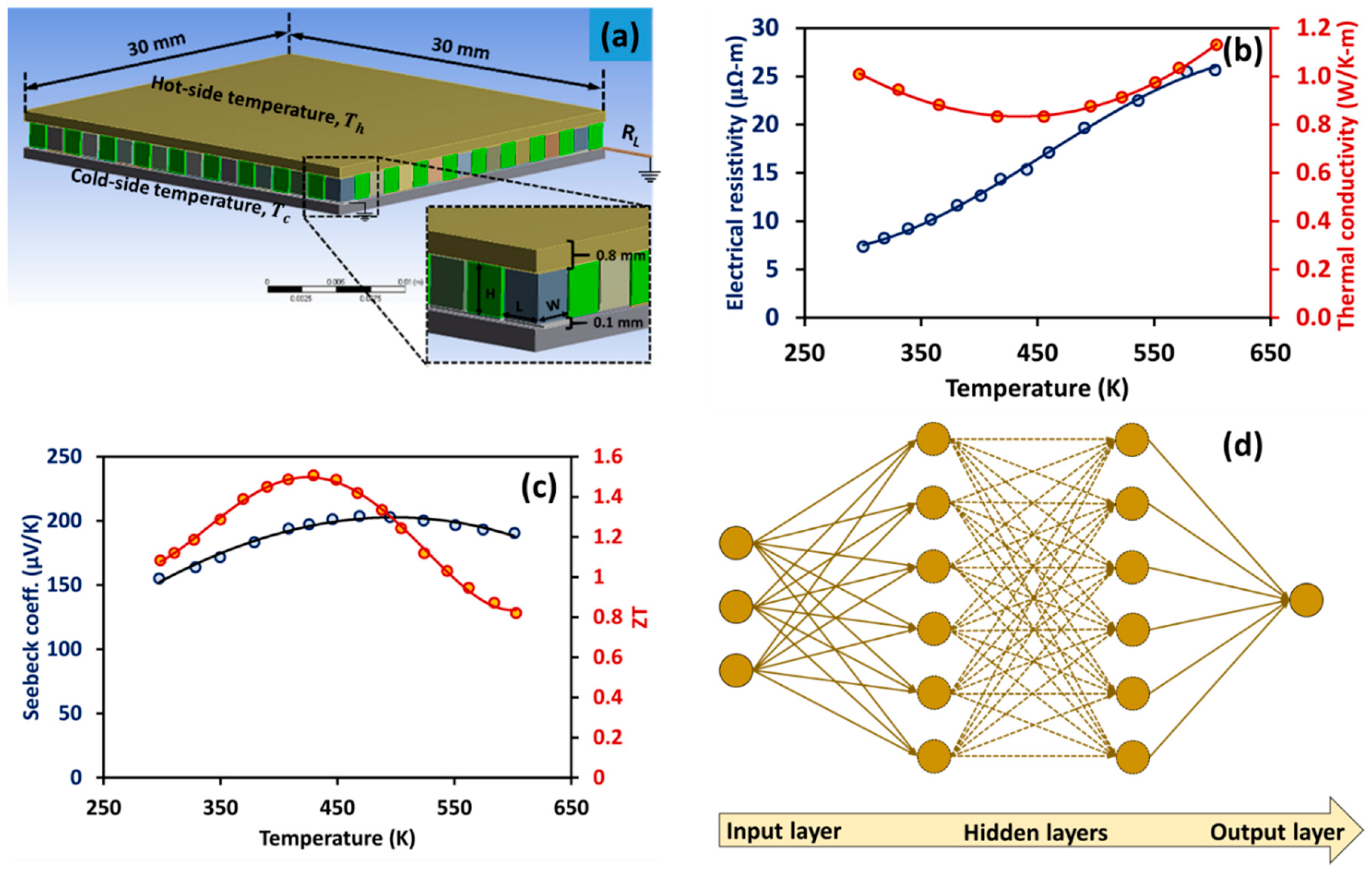
Figure 2a shows the computer-aided design model of the TEG module. It has an overall dimension of 30 × 30 × 3.5 mm3. A number of p–n legs of varying sizes are assembled electrically in a series and thermally in parallel using copper electrodes of 0.1-mm thickness. Ceramic substrates are added on both sides to electrically isolate the TEG module. The hot-side temperature is fixed at 513 K, and the cold-side temperature is fixed at 295 K. We have considered the state-of-the-art bismuth telluride alloy, Bi0.5Sb1.5−xCuxTe3, x = 0.005 [55], as the working material in this study. Figure 2b,c depicts the temperature-dependent thermal conductivity, electrical resistivity, Seebeck coefficient, and ZT of the TE material.
Table 1 shows the range of the input parameters—leg length, leg area, and resistive load—considered in this study. We have not considered any interaction effect among the input parameters, as each of these parameters has an independent effect on TEG performance. The internal electrical and thermal resistances depend on leg area and length, independently. In addition, the external resistive load is varied independent of the leg dimensions. As mentioned in Section 2.3, we used a total of 53 = 125 data points with 75 random data points used for training, and the remaining 50 data points divided equally for validation and testing. The output variables for each input combination—power and efficiency—were obtained using the finite element method, as described in Section 2. Figure 2d shows the architecture of the artificial neural network model used in this study.
Figure 3a,c compares the raw data for power and efficiency of the TEG module against results obtained using ANN models with two, four, and six neurons per hidden layer. It is noted that as the number of neurons is increased, the difference between the raw data and model data decreases. This is evident from Figure 3b,d, which depicts the RMSE (calculated for all 125 data points) versus the number of neurons for power and efficiency, respectively. Increasing the number of neurons from one to 10, the RMSE first decreases drastically, and then it almost saturates after six neurons. With six neurons in each of the hidden layers, the RMSE for power was found to be less than 0.1 W, and the RMSE for efficiency was found to be less than 0.2%. Therefore, all of the results presented in the remaining part of this study were obtained with six neurons per hidden layer.
On a 64-bit computer (with 8.0 GB RAM and 2.79 GHz processor), training, testing, and validating the selected ANN model took approximately 6.8 s. However, once the model was trained, predicting the TEG performance for a “what if” set of input variables took only 26.4 ms. Performing a parametric study using ANSYS v17.0 on the same computer, on the other hand, required about 6.0 min to simulate one data point. As suggested by Subbarayan et al. [38] and Marwah et al. [61], ANN is an efficient and powerful tool for predicting the TEG performance almost in real-time. This clearly signifies the importance of the ANN model in a manufacturing setting, where real-time decisions need to be made.
3.1. Effect of Leg Cross-Sectional Area on TEG Performance
TEG legs are typically square in a cross-section; therefore, for simplicity, we have considered leg width instead of the cross-sectional area in this section. Figure 4a–e depicts the effect of varying the leg width on the output power at different leg lengths and resistive loads. The markers denote raw data, and the dotted lines denote the predictions using the ANN model having two hidden layers with six neurons. Figure 4f shows the RMSE, which is below 0.1 W for all of the data points for power. It can also be noted that at a fixed leg length and resistive load, power first increases with an increase in leg width, reaches a maximum value, and then decreases with a further increase in leg width. The optimal leg width can be seen to be 1.5 mm (i.e., the optimal leg cross-sectional area is 1.5 mm × 1.5 mm), and it is almost independent of leg length.
Figure 5a–e depicts the effect of varying the leg width on the TEG efficiency at different leg lengths and resistive loads. Figure 5f shows the RMSE, which is below 0.2% for all of the data points for efficiency. It can also be noted that at the fixed leg length and resistive load, efficiency first increases with the increase in leg width, reaches a maximum value, and then decreases with any further increase in leg width. Similar to power, the optimal leg width for efficiency can be seen to occur at 1.5 mm (i.e., cross-sectional area: 1.5 mm × 1.5 mm).
3.2. Effect of Leg Length on TEG Performance
Figure 6 depicts the effect of varying the leg length on the output power for different leg areas and resistive loads. It can be noted that, unlike for the cross-sectional area, the power versus leg length curves are relatively flat, indicating that leg length does not have a prominent effect on the power. For a small cross-sectional area (i.e., 1 mm × 1 mm), power slowly decreases as the leg length increases; however, for a large cross-sectional area (i.e., 2 mm × 2 mm), power slowly increases with as the leg length increases. The optimal leg length can be seen to change with any change in the cross-sectional area. At the optimal leg area of 1.5 mm × 1.5 mm and a resistive load of 4 Ω, leg length has a minor effect on power. The highest power exists at an optimal leg length of 1.5 mm, which is same as the optimal length width, indicating that the optimal TEG leg is a cube.
Figure 7 depicts the effect of varying the leg length on the TEG efficiency for different leg areas and resistive loads. It can also be noted that, unlike power, the effect of leg length on efficiency is more pronounced. In most cases, at a fixed cross-sectional area and resistive load, efficiency can be seen to increase with any increase in leg length. The highest efficiency occurs at a leg area of 1.5 mm × 1.5 mm and a leg length of 2 mm. This implies that TEG power is highest when legs are cubical, while TEG efficiency is maximum when legs are cuboidal.
3.3. Effect of Resistive Load on TEG Performance
Figure 8 and Figure 9 depict the effect of resistive load on power and efficiency, respectively, at fixed leg cross-sectional areas and lengths. As shown in Figure 8f and Figure 9f, the RMSE for both the cases is small, indicating that the predictions of the ANN model and the raw data are in excellent agreement. Both the power and efficiency curves show similar trends. Increasing the load resistance at small leg areas (below 1.25 mm × 1.25 mm) increases the power and efficiency. At a leg area above 1.75 mm × 1.75 mm, the power and efficiency decrease with any increase in load resistance. The maximum power of 4.4 W occurs when the resistive load is equal to 4 Ω at the optimal leg area of 1.5 mm × 1.5 mm and leg length of 1.5 mm. The maximum efficiency of 6.4% can be found to occur when the resistive load is equal to 6 Ω at the optimal leg area of 1.5 mm × 1.5 mm and leg length of 2 mm.
3.4. Comparing ANN Predictions with Prior Studies
The optimal geometric parameters and resistive load obtained in this study are in agreement with the trends reported in prior studies. Theoretically, designing a TEG for maximum power relies on an optimization of thermal resistance versus electrical resistance. Increasing the leg length and/or decreasing the leg cross-sectional area increases the internal thermal resistance; however, it also increases the internal electrical resistance. Few studies have suggested that the TEG power is maximum when the module internal electrical resistance matches the load resistance [64] and the internal thermal resistance due to the active thermoelectric layers is close to the external thermal resistance (due to the inactive layers such as substrates and heat sinks) [20]. The thermal-to-electrical conversion efficiency, on the other hand, has been reported to increase with any increase in the internal-to-external thermal resistance ratio [20]. Clearly, the optimal geometric parameters and resistive load for the maximum power and the maximum efficiency are not the same, which is in agreement with the results obtained in this study. Rowe et al. [24,64] reported that at a fixed temperature difference, the TEG efficiency can be improved by increasing the leg length; however, the TEG power is not maximum when very long legs are employed. Therefore, the optimal leg length is usually a compromise between the required power and the acceptable conversion efficiency [24]. Unlike leg length, the effect of the leg cross-sectional area on TEG performance is not straightforward. For a given size of TEG module, changing the leg area changes not only the internal thermal and electrical resistances, it also affects the number of legs. In additional, varying the leg area causes a variation in contact resistances between TEG legs and copper electrodes as well as the exposed surface area for the thermal losses. The optimal leg area has been also found to be somewhere in between two extreme values [19,20].
4. Conclusions
The major findings of the paper are summarized below:
- An ANN model that has two hidden layers with six neurons in each layer can predict TEG performance with a great degree of accuracy. Increasing the number of neurons above six does not improve the model accuracy, as the root mean square error almost saturates after six neurons.
- The predicted power was found to be within ±0.1 W, and efficiency was found to be within ±0.2%.
- The trained ANN model required only 26.4 ms per data point for predicting TEG performance against the 6.0 min needed by the traditional numerical simulations.
- There exists an optimal TEG leg cross-sectional area where power and efficiency are maximum.
- The effect of leg length on power is not as prominent as the cross-sectional area, although an optimal leg length exists. Efficiency was found to increase with an increase in leg length.
- Under a given range of leg dimensions, TEG was found to have maximum power when legs are cubical (1.5 × 1.5 × 1.5 mm3). On the other hand, the TEG efficiency was found to be maximum when legs are cuboidal (1.5 × 1.5 × 2 mm3) at a resistive load of 6 Ω.
Author Contributions
R.A.K. and R.L.M. conceived the idea. R.A.K. performed modeling and simulations. R.L.M. and S.P. supervised the research. All authors contributed discussion and wrote the manuscript.
Acknowledgments
S.P. acknowledges the financial support from DARPA MATRIX program. R.A.K. was supported through Army SBIR program and ICTAS Doctoral Scholarship.
Conflicts of Interest
There is no conflict of interest to declare.
Nomenclature
| TE | Thermoelectric |
| TEG | Thermoelectric Generator |
| ZT | Figure of merit |
| ANN | Artificial neural network |
| FEA | Finite element analysis |
| T | Temperature |
| Ap | Cross-sectional area of p-type leg |
| An | Cross-sectional area of n-type leg |
| Lp | Length of p-type leg |
| Ln | Length of n-type leg |
| N | Number of thermocouples |
| I | Electric current |
| R | Electrical load |
| ∆T | Temperature difference |
| Electrical conductivity | |
| κ | Thermal conductivity |
| Electrical resistivity | |
| S | Seebeck coefficient |
| Open circuit voltage | |
| Module output voltage | |
| Hot side temperature | |
| Cold side temperature | |
| Seebeck coefficients (p-type material) | |
| Seebeck coefficients (n-type material) | |
| Seebeck coefficients (thermocouple) | |
| π | Peltier coefficient |
| Rate of thermal energy absorbed | |
| Rate of thermal energy released | |
| Internal electrical resistance | |
| Internal thermal conductance | |
| Output power | |
| Heat flux vector | |
| Current density vector | |
| Electric field intensity | |
| Specific heat matrix | |
| Dielectric permittivity coefficient matrix | |
| Thermal conductivity matrix | |
| Seebeck coefficient coupling matrix | |
| Electrical conductivity coefficient matrix | |
| Nodal temperature vector | |
| Nodal electric potential vector | |
| Heat flow vectors | |
| Peltier heat load vector | |
| Nodal current vector | |
| Output vector in kth layer | |
| Activation function | |
| Connection weight matrices | |
| Bias weight matrices | |
| J | Jacobian matrix |
| i | Number of iteration steps |
| e | Network errors |
| Mean-square error | |
| Root-mean-square error |
References
- Vining, C.B. An inconvenient truth about thermoelectrics. Nat. Mater. 2009, 8, 83–85. [Google Scholar] [CrossRef] [PubMed]
- Junior, O.H.A.; Calderon, N.H.; de Souza, S.S. Characterization of a thermoelectric generator (TEG) system for waste heat recovery. Energies 2018, 11, 1555. [Google Scholar] [CrossRef]
- Kishore, R.A.; Sanghadasa, M.; Priya, S. Optimization of segmented thermoelectric generator using taguchi and anova techniques. Sci. Rep. 2017, 7, 16746. [Google Scholar] [CrossRef] [PubMed]
- Anant Kishore, R.; Kumar, P.; Sanghadasa, M.; Priya, S. Taguchi optimization of bismuth-telluride based thermoelectric cooler. J. Appl. Phys. 2017, 122, 025109. [Google Scholar] [CrossRef]
- Teffah, K.; Zhang, Y.; Mou, X.-L. Modeling and experimentation of new thermoelectric cooler—Thermoelectric generator module. Energies 2018, 11, 576. [Google Scholar] [CrossRef]
- Zhang, C.-W.; Xu, K.-J.; Li, L.-Y.; Yang, M.-Z.; Gao, H.-B.; Chen, S.-R. Study on a battery thermal management system based on a thermoelectric effect. Energies 2018, 11, 279. [Google Scholar] [CrossRef]
- Lee, P.-Y.; Lin, P.-H. Evolution of thermoelectric properties of Zn4Sb3 prepared by mechanical alloying and different consolidation routes. Energies 2018, 11, 1200. [Google Scholar] [CrossRef]
- Liu, R.; Ren, G.; Tan, X.; Lin, Y.; Nan, C. Enhanced thermoelectric properties of Cu3SbSe3-based composites with inclusion phases. Energies 2016, 9, 816. [Google Scholar] [CrossRef]
- Lin, C.-K.; Chen, M.-S.; Huang, R.-T.; Cheng, Y.-C.; Lee, P.-Y. Thermoelectric properties of alumina-doped Bi0.4Sb1.6Te3 nanocomposites prepared through mechanical alloying and vacuum hot pressing. Energies 2015, 8, 12573–12583. [Google Scholar] [CrossRef]
- Elsheikh, M.H.; Shnawah, D.A.; Sabri, M.F.M.; Said, S.B.M.; Hassan, M.H.; Bashir, M.B.A.; Mohamad, M. A review on thermoelectric renewable energy: Principle parameters that affect their performance. Renew. Sustain. Energy Rev. 2014, 30, 337–355. [Google Scholar] [CrossRef]
- Xie, D.; Xu, J.; Liu, G.; Liu, Z.; Shao, H.; Tan, X.; Jiang, J.; Jiang, H. Synergistic optimization of thermoelectric performance in P-type Bi0.48Sb1.52Te3/graphene composite. Energies 2016, 9, 236. [Google Scholar] [CrossRef]
- Harman, T.; Walsh, M.; Turner, G. Nanostructured thermoelectric materials. J. Electron. Mater. 2005, 34, L19–L22. [Google Scholar] [CrossRef]
- Venkatasubramanian, R.; Silvola, E.; Colpitts, T.; O’quinn, B. Thin-film thermoelectric devices with high room-temperature figures of merit. In Materials for Sustainable Energy: A Collection of Peer-Reviewed Research and Review Articles from Nature Publishing Group; World Scientific: Singapore, 2011; pp. 120–125. [Google Scholar]
- Hsu, K.F.; Loo, S.; Guo, F.; Chen, W.; Dyck, J.S.; Uher, C.; Hogan, T.; Polychroniadis, E.; Kanatzidis, M.G. Cubic AgPbmSbTe2+m: Bulk thermoelectric materials with high figure of merit. Science 2004, 303, 818–821. [Google Scholar] [CrossRef] [PubMed]
- Hu, X.; Jood, P.; Ohta, M.; Kunii, M.; Nagase, K.; Nishiate, H.; Kanatzidis, M.G.; Yamamoto, A. Power generation from nanostructured PbTe-based thermoelectrics: Comprehensive development from materials to modules. Energy Environ. Sci. 2016, 9, 517–529. [Google Scholar] [CrossRef]
- Chen, J.; Li, K.; Liu, C.; Li, M.; Lv, Y.; Jia, L.; Jiang, S. Enhanced efficiency of thermoelectric generator by optimizing mechanical and electrical structures. Energies 2017, 10, 1329. [Google Scholar] [CrossRef]
- Li, S.; Lam, K.H.; Cheng, K.W.E. The thermoelectric analysis of different heat flux conduction materials for power generation board. Energies 2017, 10, 1781. [Google Scholar] [CrossRef]
- Yazawa, K.; Shakouri, A. Optimization of power and efficiency of thermoelectric devices with asymmetric thermal contacts. J. Appl. Phys. 2012, 111, 024509. [Google Scholar] [CrossRef]
- Montecucco, A.; Siviter, J.; Knox, A.R. Constant heat characterisation and geometrical optimisation of thermoelectric generators. Appl. Energy 2015, 149, 248–258. [Google Scholar] [CrossRef]
- Dunham, M.T.; Barako, M.T.; LeBlanc, S.; Asheghi, M.; Chen, B.; Goodson, K.E. Power density optimization for micro thermoelectric generators. Energy 2015, 93, 2006–2017. [Google Scholar] [CrossRef] [Green Version]
- Kumar, S.; Heister, S.D.; Xu, X.; Salvador, J.R. Optimization of thermoelectric components for automobile waste heat recovery systems. J. Electron. Mater. 2015, 44, 3627–3636. [Google Scholar] [CrossRef]
- Sahin, A.Z.; Yilbas, B.S. The thermoelement as thermoelectric power generator: Effect of leg geometry on the efficiency and power generation. Energy Convers. Manag. 2013, 65, 26–32. [Google Scholar] [CrossRef]
- Yilbas, B.; Sahin, A. Thermoelectric device and optimum external load parameter and slenderness ratio. Energy 2010, 35, 5380–5384. [Google Scholar] [CrossRef]
- Rowe, D.; Min, G. Design theory of thermoelectric modules for electrical power generation. IEE Proc. Sci. Meas. Technol. 1996, 143, 351–356. [Google Scholar] [CrossRef]
- Mitrani, D.; Salazar, J.; Turó, A.; García, M.J.; Chávez, J.A. One-dimensional modeling of te devices considering temperature-dependent parameters using spice. Microelectron. J. 2009, 40, 1398–1405. [Google Scholar] [CrossRef]
- Wang, X.-D.; Huang, Y.-X.; Cheng, C.-H.; Lin, D.T.-W.; Kang, C.-H. A three-dimensional numerical modeling of thermoelectric device with consideration of coupling of temperature field and electric potential field. Energy 2012, 47, 488–497. [Google Scholar] [CrossRef]
- Cheng, C.-H.; Huang, S.-Y.; Cheng, T.-C. A three-dimensional theoretical model for predicting transient thermal behavior of thermoelectric coolers. Int. J. Heat Mass Transf. 2010, 53, 2001–2011. [Google Scholar] [CrossRef]
- Solarsystem.nasa.gov. Radioisotope Power Systems: Radioisotope Thermoelectric Generator. Available online: https://solarsystem.nasa.gov/missions/rps/rtg (accessed on 17 December 2017).
- Von Lukowicz, M.; Abbe, E.; Schmiel, T.; Tajmar, M. Thermoelectric generators on satellites—An approach for waste heat recovery in space. Energies 2016, 9, 541. [Google Scholar] [CrossRef]
- Green Car Congress. BMW Provides An Update on Waste Heat Recovery Projects; Turbosteamer and the Thermoelectric Generator. Available online: http://www.greencarcongress.com/2011/08/bmwthermal-20110830.html (accessed on 17 December 2017).
- Mirhosseini, M.; Rezaniakolaei, A.; Rosendahl, L. Numerical study on heat transfer to an arc absorber designed for a waste heat recovery system around a cement kiln. Energies 2018, 11, 671. [Google Scholar] [CrossRef]
- Li, Z.; Li, W.; Chen, Z. Performance analysis of thermoelectric based automotive waste heat recovery system with nanofluid coolant. Energies 2017, 10, 1489. [Google Scholar] [CrossRef]
- Cheng, K.; Feng, Y.; Lv, C.; Zhang, S.; Qin, J.; Bao, W. Performance evaluation of waste heat recovery systems based on semiconductor thermoelectric generators for hypersonic vehicles. Energies 2017, 10, 570. [Google Scholar] [CrossRef]
- Candle Powered Teg (Teg-Can-1). Available online: http://www.tegmart.com/diy-teg-kits/diy-candle-powered-teg-with-led-options/ (accessed on 17 December 2017).
- 10 Watt Direct Flame Thermoelectric Generator (Aka “Camp Teg”). Available online: http://www.tegpower.com/pro2.htm (accessed on 17 December 2017).
- Duran, O.; Capaldo, A.; Duran Acevedo, P.A. Lean maintenance applied to improve maintenance efficiency in thermoelectric power plants. Energies 2017, 10, 1653. [Google Scholar] [CrossRef]
- Digi-Key. Energy Harvesting in the Smart Grid. 2015. Available online: https://www.digikey.com/en/articles/techzone/2015/sep/energy-harvesting-in-the-smart-grid (accessed on 17 January 2018).
- Subbarayan, G.; Li, Y.; Mahajan, R.L. Reliability simulations for solder joints using stochastic finite element and artificial neural network models. Trans. Am. Soc. Mech. Eng. J. Electron. Packag. 1996, 118, 148–156. [Google Scholar] [CrossRef]
- Mahajan, R.L.; Wang, X. Neural network models for thermally based microelectronic manufacturing processes. J. Electrochem. Soc. 1993, 140, 2287–2293. [Google Scholar] [CrossRef]
- Li, Y.; Mahajan, R.L.; Nikmanesh, N. Fine pitch stencil printing process modeling and optimization. J. Electron. Packag. 1996, 118, 1–6. [Google Scholar] [CrossRef]
- Calmidi, V.; Mahajan, R.L. Optimization for thermal and electrical performance for a flip-chip package using physical-neural network modeling. In Proceedings of the 47th Electronic Components and Technology Conference, San Jose, CA, USA, 18–21 May 1997; pp. 1163–1169. [Google Scholar]
- Ang, Z.Y.A.; Woo, W.L.; Mesbahi, E. Artificial neural network based prediction of energy generation from thermoelectric generator with environmental parameters. J. Clean Energy Technol. 2017, 5, 458–463. [Google Scholar] [CrossRef]
- Ang, Z.Y.A.; Woo, W.L.; Mesbahi, E. Prediction and analysis of energy generation from thermoelectric energy generator with operating environmental parameters. In Proceedings of the 2017 International Conference on Green Energy and Applications (ICGEA), Singapore, 25–27 March 2017; pp. 80–84. [Google Scholar]
- Ciylan, B. Determination of output parameters of a thermoelectric module using artificial neural networks. Electron. Electr. Eng. 2011, 116, 63–66. [Google Scholar] [CrossRef]
- Goldsmid, H.J. Introduction to Thermoelectricity; Springer: Berlin, Germany, 2010; Volume 121. [Google Scholar]
- Rowe, D.M. Thermoelectrics Handbook: Macro to Nano; CRC Press: Boca Raton, FL, USA, 2005. [Google Scholar]
- Zheng, X.; Liu, C.; Yan, Y.; Wang, Q. A review of thermoelectrics research—Recent developments and potentials for sustainable and renewable energy applications. Renew. Sustain. Energy Rev. 2014, 32, 486–503. [Google Scholar] [CrossRef]
- Zhu, W.; Deng, Y.; Wang, Y.; Wang, A. Finite element analysis of miniature thermoelectric coolers with high cooling performance and short response time. Microelectron. J. 2013, 44, 860–868. [Google Scholar] [CrossRef]
- Kishore, R.A.; Kumar, P.; Priya, S. A comprehensive optimization study on Bi2Te3-based thermoelectric generators using the taguchi method. Sustain. Energy Fuels 2018, 2, 175–190. [Google Scholar] [CrossRef]
- ANSYS. Ansys Mechanical Apdl Theory Reference; ANSYS Inc.: Canonsburg, PA, USA, 2012. [Google Scholar]
- Mengali, O.; Seiler, M. Contact resistance studies on thermoelectric materials. Adv. Energy Convers. 1962, 2, 59–68. [Google Scholar] [CrossRef]
- Högblom, O.; Andersson, R. Analysis of thermoelectric generator performance by use of simulations and experiments. J. Electron. Mater. 2014, 43, 2247–2254. [Google Scholar] [CrossRef]
- Chen, W.-H.; Wang, C.-C.; Hung, C.-I. Geometric effect on cooling power and performance of an integrated thermoelectric generation-cooling system. Energy Convers. Manag. 2014, 87, 566–575. [Google Scholar] [CrossRef]
- Astrain, D.; Vián, J.; Martínez, A.; Rodríguez, A. Study of the influence of heat exchangers’ thermal resistances on a thermoelectric generation system. Energy 2010, 35, 602–610. [Google Scholar] [CrossRef]
- Hao, F.; Qiu, P.; Tang, Y.; Bai, S.; Xing, T.; Chu, H.-S.; Zhang, Q.; Lu, P.; Zhang, T.; Ren, D. High efficiency Bi2Te3-based materials and devices for thermoelectric power generation between 100 and 300 °C. Energy Environ. Sci. 2016, 9, 3120–3127. [Google Scholar] [CrossRef]
- Schalkoff, R.J. Artificial Neural Networks; McGraw-Hill: New York, NY, USA, 1997; Volume 1. [Google Scholar]
- McGonagle, J. Feedforward Neural Networks. Available online: https://brilliant.Org/wiki/feedforward-neural-networks/ (accessed on 18 December 2017).
- MathWorks. Create, Configure, and Initialize Multilayer Neural Networks. Available online: https://www.mathworks.com/help/nnet/ug/create-configure-and-initialize-multilayer-neural-networks.html (accessed on 19 December 2017).
- MathWorks. Levenberg-Marquardt Algorithm. Available online: https://www.mathworks.com/help/nnet/ref/trainlm.html (accessed on 20 December 2017).
- MathWorks. Improve Neural Network Generalization and Avoid Overfitting. Available online: https://www.mathworks.com/help/nnet/ug/improve-neural-network-generalization-and-avoid-overfitting.html (accessed on 18 December 2017).
- Marwah, M.; Li, Y.; Mahajan, R.L. Integrated neural network modeling for electronic manufacturing. J. Electron. Manuf. 1996, 6, 79–91. [Google Scholar] [CrossRef]
- Watson, P.; Gupta, K.; Mahajan, R.L. Applications of knowledge-based artificial neural network modeling to microwave components. Int. J. RF Microw. Comput. Aided Eng. 1999, 9, 254–260. [Google Scholar] [CrossRef]
- Marwah, M.; Mahajan, R.L. Building neural network equipment models using model modifier techniques. IEEE Trans. Semicond. Manuf. 1999, 12, 377–381. [Google Scholar] [CrossRef]
- Rowe, D.; Min, G. Evaluation of thermoelectric modules for power generation. J. Power Sources 1998, 73, 193–198. [Google Scholar] [CrossRef]
Figure 1.
Comparison between the numerical and experimental results for (a) output power and (b) efficiency. The cold-side temperature is fixed at 295 K.
Figure 1.
Comparison between the numerical and experimental results for (a) output power and (b) efficiency. The cold-side temperature is fixed at 295 K.

Figure 2.
(a) Thermoelectric generator (TEG) module with key geometric dimensions and boundary conditions. (b) Thermal and electrical properties of the thermoelectric (TE) material. (c) The Seebeck coefficient and ZT of the TE material. Figure (b) and (c) are constructed using the temperature-dependent TE material information available in Hao et al. [55]. (d) The architecture of the artificial neural network model.

Figure 3.
Comparison of raw data versus ANN predictions. (a) Raw data versus ANN data with two, four, and six neurons for power. The difference between the two kinds of data decreases with the increase in the number of neurons. (b) Root mean square error (RMSE) for power versus number of neurons. The RMSE for power first decreases with an increase in the number of neurons, but it almost saturates beyond six neurons. (c) Raw data versus ANN data with two, four, and six neurons for efficiency. The difference between the two kinds of data decreases as the number of neurons increases. (d) Root mean square error (RMSE) for efficiency versus number of neurons. RMSE for efficiency first decreases as the number of neurons increases, but it almost saturates beyond six neurons.

Figure 4.
The effect of varying the leg width on the output power for different leg lengths and resistive loads. (a) Power versus leg width for a leg length of 1 mm at different resistive loads. (b) Power versus leg width for a leg length of 1.25 mm at different resistive loads. (c) Power versus leg width for a leg length of 1.5 mm at different resistive loads. (d) Power versus leg width for a leg length of 1.75 mm at different resistive loads. (e) Power versus leg width for a leg length of 2 mm at different resistive loads. (f) RMSE for power.

Figure 5.
The effect of varying the leg width on the efficiency for different leg length and resistive load. (a) Efficiency versus leg width for a leg length of 1 mm at different resistive loads. (b) Efficiency versus leg width for a leg length of 1.25 mm at different resistive loads. (c) Efficiency versus leg width for a leg length of 1.5 mm at different resistive loads. (d) Efficiency versus leg width for a leg length of 1.75 mm at different resistive loads. (e) Efficiency versus leg width for a leg length of 2 mm at different resistive loads. (f) RMSE for efficiency.

Figure 6.
The effect of varying the leg length on the output power for different leg widths and resistive loads. (a) Power versus leg length for a leg area of 1 mm × 1 mm at different resistive loads. (b) Power versus leg length for a leg area of 1.25 mm × 1.25 mm at different resistive loads. (c) Power versus leg length for a leg area of 1.5 mm × 1.5 mm at different resistive loads. (d) Power versus leg length for a leg area of 1.75 mm × 1.75 mm at different resistive loads. (e) Power versus leg length for a leg area of 2 mm × 2 mm at different resistive loads. (f) RMSE for power.

Figure 7.
The effect of varying the leg length on efficiency for different leg areas and resistive loads. (a) Efficiency versus leg length for a leg area of 1 mm × 1 mm at different resistive loads. (b) Efficiency versus leg length for a leg area of 1.25 mm × 1.25 mm at different resistive loads. (c) Efficiency versus leg length for a leg area of 1.5 mm × 1.5 mm at different resistive loads. (d) Efficiency versus leg length for a leg area of 1.75 mm × 1.75 mm at different resistive loads. (e) Efficiency versus leg length for a leg area of 2 mm × 2 mm at different resistive loads. (f) RMSE for Efficiency.

Figure 8.
The effect of varying the resistive load on the output power for different leg widths and leg lengths. (a) Power versus resistive load for a leg area of 1 mm × 1 mm at different leg lengths. (b) Power versus resistive load for a leg area of 1.25 mm × 1.25 mm at different leg lengths. (c) Power versus resistive load for a leg area of 1.5 mm × 1.5 mm at different leg lengths. (d) Power versus resistive load for a leg area of 1.75 mm × 1.75 mm at different leg lengths. (e) Power versus resistive load for a leg area of 2 mm × 2 mm at different leg lengths. (f) RMSE for power.

Figure 9.
The effect of varying the resistive load on efficiency for different leg widths and leg lengths. (a) Efficiency versus resistive load for a leg area of 1 mm × 1 mm at different leg lengths. (b) Efficiency versus resistive load for a leg area of 1.25 mm × 1.25 mm at different leg lengths. (c) Efficiency versus resistive load for a leg area of 1.5 mm × 1.5 mm at different leg lengths. (d) Efficiency versus resistive load for a leg area of 1.75 mm × 1.75 mm at different leg lengths. (e) Efficiency versus resistive load for a leg area of 2 mm × 2 mm at different leg lengths. (f) RMSE for efficiency.


Table 1.
Range of input parameters considered for the artificial neural network (ANN) model for Thermoelectric generator (TEG).
Table 1.
Range of input parameters considered for the artificial neural network (ANN) model for Thermoelectric generator (TEG).
| Input Parameters | Range | |||||
|---|---|---|---|---|---|---|
| (A) | Leg length (mm) | 1.0 | 1.25 | 1.5 | 1.75 | 2.0 |
| (B) | Leg cross-sectional area (mm2) | 1.0 × 1.0 | 1.25 × 1.25 | 1.5 × 1.5 | 1.75 × 1.75 | 2.0 × 2.0 |
| (C) | External resistance (Ω) | 2.0 | 4.0 | 6.0 | 8.0 | 10.0 |
© 2018 by the authors. Licensee MDPI, Basel, Switzerland. This article is an open access article distributed under the terms and conditions of the Creative Commons Attribution (CC BY) license (http://creativecommons.org/licenses/by/4.0/).
Share and Cite
MDPI and ACS Style
Kishore, R.A.; Mahajan, R.L.; Priya, S. Combinatory Finite Element and Artificial Neural Network Model for Predicting Performance of Thermoelectric Generator. Energies 2018, 11, 2216. https://doi.org/10.3390/en11092216
AMA Style
Kishore RA, Mahajan RL, Priya S. Combinatory Finite Element and Artificial Neural Network Model for Predicting Performance of Thermoelectric Generator. Energies. 2018; 11(9):2216. https://doi.org/10.3390/en11092216
Chicago/Turabian StyleKishore, Ravi Anant, Roop L. Mahajan, and Shashank Priya. 2018. "Combinatory Finite Element and Artificial Neural Network Model for Predicting Performance of Thermoelectric Generator" Energies 11, no. 9: 2216. https://doi.org/10.3390/en11092216
Note that from the first issue of 2016, this journal uses article numbers instead of page numbers. See further details here.