Hydrodynamic Analysis of a Marine Current Energy Converter for Profiling Floats

Abstract

With the continuous improvement of people’s interest in ocean exploration, research on deep-water profiling floats has received more and more attention. Energy supply is the key factor that restricts the working hours of deep-water floats. For this consideration, a marine current energy converter for deep-water profiling floats is proposed in this paper. A spiral involute blade is designed so that energy can be captured in two directions. Specifically, in the shallow sea area, the energy of the radial current is captured, and in the deep-sea area, the axial relative flow energy of the floats’ autonomous up and down motions is captured. This captured energy is then converted into electrical energy to charge the battery and extend the working time of the floats. The novel spiral involute blade has unique hydrodynamic characteristics. The turbine’s self-starting performance and its capacity coefficient are the main research topics studied using the computational fluid dynamics technique. Through numerical analysis and simulation, the self-starting response range and energy capture were obtained. This paper verifies the feasibility of this innovative idea using a theory analysis and provides the basis for future prototype testing and further applied research.

1. Introduction

Since entering the 21st century, many countries have shifted their strategic focus to the oceans. United States proposed the establishment of Integrated Ocean Observing System (IOOS) [1,2], the European Union proposed the “Leader SHIP 2020” initiative [3], the United Kingdom proposed the “Oceans 2025” plan [4], and China implemented the “Strengthening Marine Powers” strategy [5], and so on. The implementation and realization of these marine strategies cannot be separated from the three-dimensional observation of oceans with marine observation equipment. As of 2016, there were more than 20 types of profiling floats in normal operation, mainly designed by the United States and France [6], and their maximum profile depth was mainly concentrated at about 2000 m.

However, the vast ocean far from the mainland has a depth of more than 2000 m, and the average depth of the global ocean reaches 3850 m. In the North Atlantic, the temperature and salinity relationship at 2000 m changes rapidly, and it is very difficult to use a delay mode correction for the data obtained from the profiling floats [7]. It can be seen that it is necessary to extend the observation depth of the automatic profiling floats to obtain deeper observational data. At present, the international deep-sea automatic profiling floats mainly include Deep Sounding Oceanographic Lagrangian Observer (Deep-SOLO), developed by the Scripps Institution of Oceanography, and Autonomous Profiling Explorer Deep (APEX-Deep), developed by Teledyne Webb [8,9], with a maximum dive depth of 6000 m. In 2017, our team successfully developed the 4000-m deep-sea Argo profiling float and conducted a sea trial in the Mariana Trench (as shown in Figure 1).

However, as the operational depth of floats increases, the required energy increases significantly, and due to the corresponding increase in the environmental pressure, the wall thickness of the float shell must be increased in order to meet the pressure requirements, resulting in an increase in mass and volume. As a result, the energy consumption of the device is increased. Traditional battery systems are large and have limited capacity. Lithium batteries also have the potential risk of contaminating the marine environment. Therefore, we have adopted high-efficiency hydraulic pump buoyancy drive technology and proposed an innovative concept for integrated ocean current energy generation. We have also added a marine energy conversion device to our existing float. The energy of the ocean current is converted into electricity to charge the battery and the working time of the buoy is extended.

The specific design concept uses a two-way energy-absorption turbine on the top of the float (as shown in Figure 2). In different water depths and sea areas, the horizontal movement of the current and the vertical movement of the float in the vertical direction can drive the rotation of the blade and convert the kinetic energy into electrical energy. In the shallow sea areas where ocean current energy density is high, the rotation of the blades is mainly driven by the horizontal currents; in the relatively calm deep-sea areas, the motion of fluids caused by the float’s autonomous bobbing and submerging movements drives the blades to rotate. To the best of our knowledge, the use of wave energy to power floats has a definite application basis, the main working principle is that the buoy of the wave energy converter vibrates up and down under the action of waves, which is then stored and converted into electrical energy sufficient for marine lighting [10,11,12]. These ocean energy converters are usually not less than two meters in diameter. We have not yet seen relevant research results on the application of ocean energy in deep-sea profiling floats, and its volume is relatively small, the characteristic diameter of the cylindrical profiling float mentioned in Figure 1 does not exceed 0.4 m. Moreover, the two-way energy capture of the turbine is also a major innovation in this paper.

This paper will mainly introduce the design and analysis of the motion and the force of the marine energy converter blades used for profiling floats and will describe a numerical simulation of the hydrodynamics to determine the feasibility and applicable conditions of the innovative application.

2. Blade Design and Analysis

As the energy capture device, the turbine blades are the most important components that need to be studied and designed. They are also the focus of this paper. Presently, there are mainly two types of turbines used in ocean energy utilization technology, classified as the horizontal axis type and the vertical axis type, according to the relative position of the flow direction and the rotation axis [13,14,15]. The blades needed in this paper can achieve energy capture in both the horizontal and vertical directions, that is, self-starting rotation and energy conversion can be realized in both the horizontal and vertical directions, so can the existing two forms of turbines be combined? To answer this question, a spiral involute blade has been designed.

2.1. Blade Design

The Indian Institute of Technology studied the helical Savonius rotor for the purpose of alleviating the problem of uneven blade torque [16]. The tidal current rotor has good self-starting characteristics and the maximum energy efficiency is about 0.18. Gorlov proposed a new spiral blade [17,18] and the Gorlov Helical Turbine Company introduced the GHT vertical axis spiral tidal turbine. The spiral blade has a specified torsion angle, good self-starting performance, and smooth operation. Ocean Renewable Power (Portland, ME, USA) has developed spiral vane turbines that adapt to different environments, such as RivGen, TidGen, and OCGen [19]. Some of these spiral vane turbines have been field-tested. All of the above previous research work applied to a vertical axis tidal current energy conversion device [20]. In our design, taking into consideration the particularity of the turbine’s bidirectional flow drive, the vertical shaft spiral involute blade was designed. The schematic diagram of the design scheme is shown in Figure 3. According to the overall size of the connected buoy, the diameter D₂ of the rotor shaft is designed to be 60 mm, the radial outer diameter D₁ is 300 mm, the axial arc length is 310 mm, the rotation angle is 30 degrees, and the involute base circle radius is r₀ = 0.233D₁. The involute equation is:

$$\{\begin{array}{l}X=r_0·\left(t_0·sin\left(t_0\right)+\cos \left(t_0\right)\right)\\ Y=r_0·\left(sin\left(t_0\right)-t_0·\cos \left(t_0\right)\right)\end{array}$$

(1)

where t₀ is the extent of the flare angle of the involute.

2.2. Movement and Stress Analysis

Taking the blade cross section as the analysis object, according to the radial flow and the axial relative flow, the force and motion analysis coordinate systems of the blade are established.

The axial relative flow conditions are shown in Figure 4a. The center point of the axis of rotation is the origin of the coordinates, and the global coordinate system OXY is established. The blade rotates counterclockwise around the axis of the turbine rotation, where the stable rotation speed is ω₁, the radius of rotation is R₁, and the positive direction of the X-axis coincides with the incoming flow direction. The local coordinate system oxy is established in the direction of the radial direction of the blade section, as shown in Figure 4a. The origin o of the local coordinate system can be determined by the radius of the blade and the angle of the blade rotation, which can be expressed as:

$${\left(X,Y\right)}_o=\left(R_1\cos \theta ,R_1\sin \theta \right)$$

(2)

where θ reflects the position of the entire blade in rotation. At any time t, there is: $\theta ={\omega }_{1}t$. Supposing the distance between any point on the blade p to o is r, then the included angle between p and the x-axis is φ and the angle between the negative direction of the x-axis and the positive direction of the X-axis is β, which is called the elevation angle. The position of any point on the blade is:

$${\left(X,Y\right)}_p=\left(R_1\cos \theta -2r\cos \left(\beta +\phi \right),\hspace{1em}{R}_1\sin \theta -2r\sin \left(\beta +\phi \right)\right)$$

(3)

The combined velocity of the blades relative to the flow is V_R1. The flow velocity V and the rotation speed of the blades around the turbine axis satisfy the following expression:

$$\stackrel{\rightharpoonup }{V_{R1}}=\stackrel{\rightharpoonup }{V}+\stackrel{\rightharpoonup }{{\omega }_1{R}_1}$$

(4)

The angle between the combined speed V_R1 and the x-axis is the angle of attack α. Therefore:

$$V_{R1}=\sqrt{V^2+{\left({\omega }_1{R}_1\right)}^2+2{\omega }_1{R}_{1}V\sin \theta }$$

(5)

$$\alpha =\mathrm{arc}\tan \left({\omega }_1{R}_1\sin \left(\beta -\theta \right)-V\cos \beta /{\omega }_1{R}_1\sin \left(\beta -\theta \right)-V\cos \beta \right)$$

(6)

Similar to the previous analysis process, for radial flow conditions shown in Figure 4b, the section perpendicular to the axis of rotation is taken as the analysis object in order to establish the coordinate system O’X’Y’, and the center point of the rotation axis is taken as the coordinate origin. Then the coordinate position of any point is:

$${\left(X{}^{\prime },Y{}^{\prime }\right)}_p=\left(R_2\cos \theta {}^{\prime }-r_2\cos \left(\theta {}^{\prime }-\phi {}^{\prime }\right),\hspace{1em}{R}_2\sin \theta {}^{\prime }-r_2\sin \left(\theta {}^{\prime }-\phi {}^{\prime }\right)\right)$$

(7)

and the combined velocity is:

$$V_{R2}=\sqrt{V^2+{\left({\omega }_2{R}_2\cos \theta {}^{\prime }\right)}^2+2V{\omega }_2{R}_2\sin \theta {}^{\prime }}$$

(8)

Generally, the direction of the drag force D in relation to the blade is the same as the direction of the combined velocity V_Ri. The lift force L is perpendicular to the drag force D, and the drag and lift are:

$$D=C_D·\frac{1}{2}\rho V_{Ri}{}^{2}S$$

(9)

$$L=C_L·\frac{1}{2}\rho V_{Ri}{}^{2}S$$

(10)

where C_D and C_L are the drag coefficient and the lift coefficient, respectively, and the values of the two are related to the position of the material of the blade and the shape and position of the blade. ρ is the density of the fluid and S is the inflow area of the blade. The vector expression of the resultant force of a single blade is:

$$\int \Delta p\left(V,\omega ,\theta \right)dS=D+L$$

(11)

where $\Delta p\left(V,\omega ,\theta \right)$ is the pressure difference between the upstream and the back surface of the blade and the differential pressure value varies with the flow velocity V, the turbine rotation speed ω, and the position angle θ. The average torque of the blade in one cycle is:

$$M_F=\frac{1}{2\pi }{\int }_0^{2\pi }T\left(\theta \right)d\theta$$

(12)

3. Hydrodynamic Performance Analysis

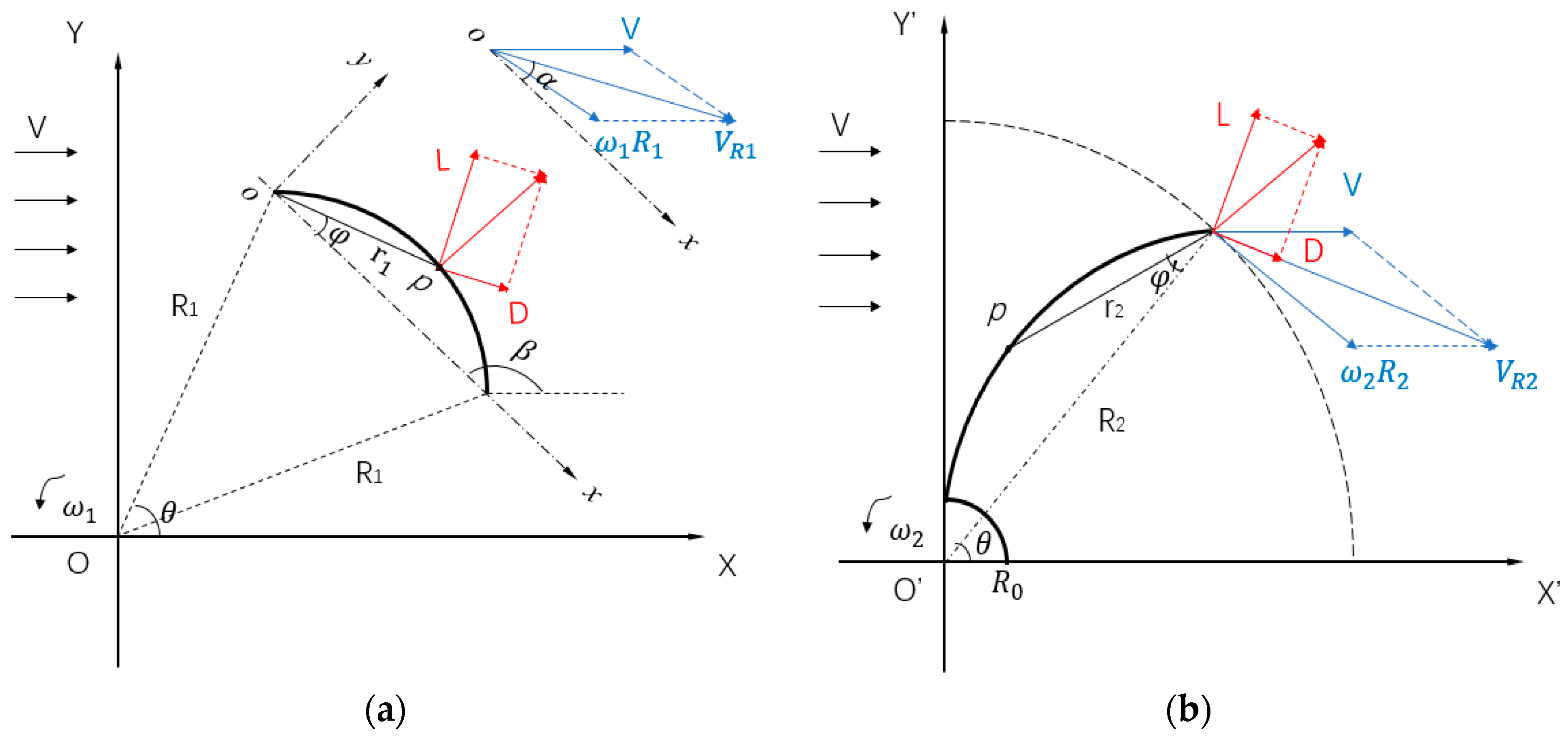
3.1. Hydrodynamic Equation

At a specific flow velocity, in addition to the hydrodynamic torque M_F, the turbine is connected to the load and the movement of the turbine can be controlled through the change of the load; this is called the load moment M_A. The turbine is also subjected to the system’s frictional resistance moment M_f. According to the D’Alembert principle and Newton’s second law of motion, the hydrodynamic equation of motion is:

$$M_F-M_A-M_f=J\frac{d\omega }{dt}$$

(13)

where J is the rotational inertia of the turbine and the effect of the frictional resistance torque is ignored in the numerical simulation. The load torque is generated by the motor and acts on the rotating shaft in the form of damping torque. According to the empirical value, the load torque is linearly related to the square of the rotational speed. The proportional coefficient of the two is represented by the load factor b.

Since the load torque and rotational angular speed of the turbine are not constant, the output power is also a function of time:

$$P={\displaystyle {\displaystyle \sum }_t}{M}_t·\omega$$

(14)

The energy utilization rate, C_p, is used to measure the turbine’s efficiency in extracting energy from currents:

$$C_p=\frac{P}{\frac{1}{2}\rho v{V}^{3}S}$$

(15)

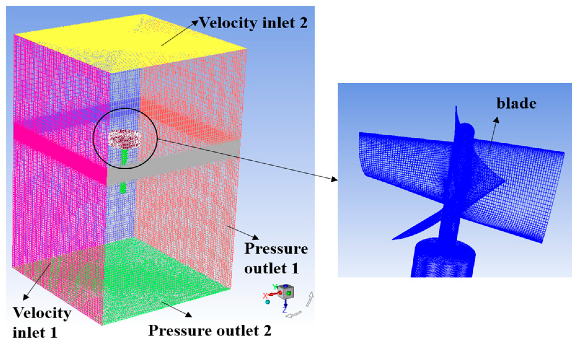
3.2. Numerical Models Establisment

The motion model equation was calculated and solved using the three-dimensional incompressible unsteady Reynolds-Averaged Navier-Stokes equation and the standard k-ε turbulence model [21]. The Reynolds average momentum equation can be expressed as follows:

$$\{\begin{array}{c}\frac{\partial \overline{u_i}}{\partial x_i}=0\\ \rho \left(\frac{\partial \overline{u_i}}{\partial t}+\overline{u_k}\frac{\partial \overline{u_i}}{\partial x_k}\right)=-\frac{\partial \overline{p}}{\partial x_i}+\frac{\partial }{\partial x_j}\left(u\frac{\partial \overline{u_i}}{\partial x_j}\right)+\frac{\partial R_{ij}}{\partial x_j}\end{array}$$

(16)

where i, j = 1, 2, 3, denotes the three spatial coordinates of xyz. The Reynolds stress tensor is defined as:

$$R_{ij}=u_T\left(\frac{\partial \overline{u_i}}{\partial x_j}+\frac{\partial \overline{u_j}}{\partial x_i}\right)-\frac{2}{3}\rho k{\delta }_{ij}$$

(17)

Several authors have proven that the standard k-ε turbulence model is suitable for solving problems involving rotating blades [22,23]. Therefore, we used this model in the present investigation.

A turbine driven by a flow current can be defined with two types of cases. In a shallow sea area, the turbine is subjected to the impact of the horizontal current, while the buoy maintains a constant velocity of 1.0 m/s. In a nearly calm deep-sea area, the turbine only moves vertically along the buoy.

A hexahedral structure grid was used to divide the grid. After the grid quality check and the grid convergence verification, the total number of final elements was 4,866,240. The grid partitioning is shown in Figure 5. In order to capture the translation and rotation response simultaneously and facilitate the mesh update, the computational domain is divided into two zones: an accompanying moving zone and a dynamic mesh zone. The accompanying moving zone around the structure is a cylindrical surface, which can follow the translational and rotational motion of the system. The rest of the computational domain is defined as a dynamic mesh zone, whose grids deform and perform any needed adaptation during the calculation. Data is transferred between the overlapping interfaces of the two zones. A User-Defined Function (UDF) was used to control the movement of the buoy and the pressure changes as the depth decreased. The specific functions are shown in Appendix A. The left and the top sections of the fluid domain are set as the velocity inlet. The left side flow velocity simulation range is set to 0.1 m/s~2.0 m/s and the upper flow velocity is kept constant at 1.0 m/s according to the designed operating speed of the profiling float. The right and the bottom sections of the fluid domain are set as pressure outlets. In order not to affect the full development of the flow field behind the turbine and reduce the flow field boundary effect, the computation domain used for simulation is a cuboid region with size of 30 D₁ × 30 D₁ × 80 D₁.

Table 1. Analysis conditions.

Description	Analysis Condition
Working fluid	Water (1025 kg/m3)
Left side velocity inlet	0.1~2.0 m/s
Upper flow velocity inlet	1.0 m/s
Pressure outlets	Relative pressure = 0 Pa

shows the computational information. The Semi-Implicit Method for Pressure Linked Equations (SIMPLE) algorithm was used for pressure-velocity coupling. All of the transport equations were discretized using the finite-volume method with a second-order upwind scheme for all transport equations [24].

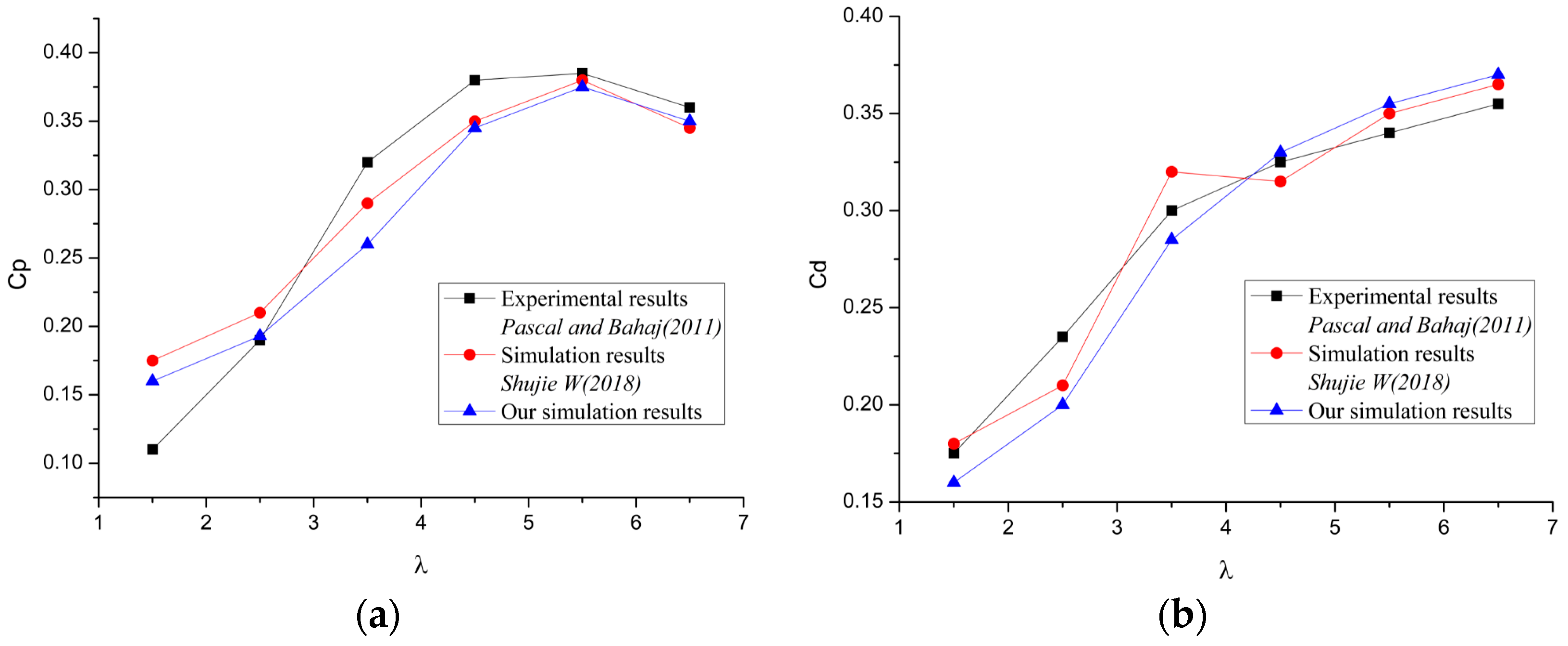
3.3. Method Validation

The numerical method used in this work has been validated against the numerical and experimental results of the study on the performance of tidal current turbines in our earlier studies [25]. In the numerical studies, tidal current turbines designed by our team compared with the experimental results observed by Pascal and Bahaj [26,27], and the free-to-rotate tidal turbine was compared with the experimental results reported in their results. The comparison of the results under the same variable parameter settings is shown in Figure 6. The numerical results coincided well with the experimental data, and the numerical method was verified to be capable of solving such a complicated issue regarding rotation and translation simultaneously.

4. Numerical Simulation Results Analysis

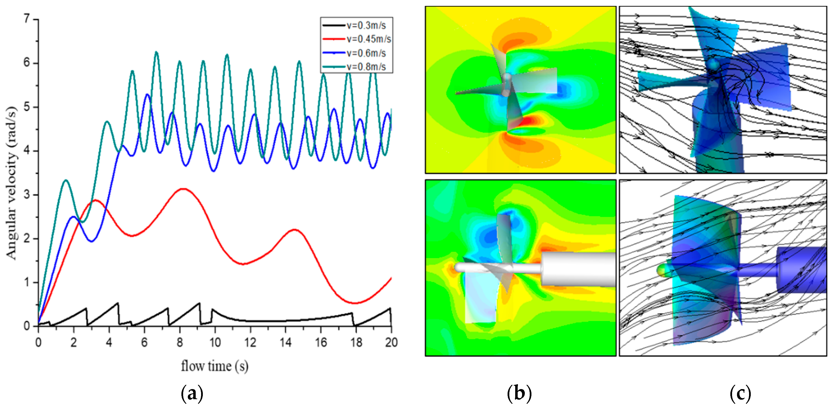
4.1. Self-Starting Analysis

The initial state of the turbine is static. With the impact of the incoming flow, when the torque of the water flow is greater than the load torque, the turbine can start to rotate. This is also the point at which the turbine suffers the largest resistance moment. Once the turbine is started, the resistance moments that are experienced during operation will become smaller than they were initially.

Figure 7 shows the time history curve of the turbine rotation angular velocity for different radial flow velocities. It can be seen that an increase of the incoming flow velocity can effectively increase the starting torque of the turbine, shorten the time of the starting phase, improve the self-starting capability, and stabilize the turbine at a higher rotational speed. When the radial flow velocity is V = 0.8 m/s, the steady rotation speed can reach 6.5 rad/s. When the flow velocity decreases to V = 0.45 m/s, the start-up time is longer, about 8 s, the impeller rotation cannot reach the periodic stable state, and the rotation changes irregularly. However, when the flow velocity is less than 0.3 m/s, the turbine is only disturbed by the water flow and has no self-starting characteristics.

Figure 8 shows the time history curve of the turbine rotation angular velocity for different load factors at flow velocity of 0.1 m/s. Different load damping coefficients mean different load moments. As can be seen from the Figure 8, the smaller the load damping coefficient, the earlier the turbine starts to stabilize. In addition, the larger the load damping coefficient, the smaller the angular velocity at which the turbine can reach the steady phase. When b = 0 N·ms²/rad², it means that there is the ideal state without load, and the angular velocity is also maximum at this time; when b = 0 N·ms²/rad² to b = 1 N·ms²/rad², the angular velocity decreases obviously. And then with the increase of b, the angular velocity value decreases slowly. It can be seen that the load plays an important role in limiting the speed of the turbine.

In addition, considering the profiling float in the actual working process, the wave and the current impact will cause the body to tilt, so that there is an angle between the turbine shaft and the direction of the flow, which will affect the self-starting performance of the turbine. Figure 9 shows the time history curve of the impeller rotation angular velocity corresponding to a flow velocity V = 0.8 m/s and body motion inclination angles β of 5°, 10°, 15°, and 20°, where the black curve represents the result of no inclination as a comparison. Due to the presence of the angle of inclination, the effective speed at which the turbine rotates is reduced, and the self-starting of the turbine at the same flow velocity is more difficult. The angular velocity variation of each rotation cycle of the impeller is greater, and the variation of the angular velocity in one cycle reaches about 5 rad/s. There are two angular velocity peaks in one rotation cycle. The calculated results show that when the range of the inclination angle does not exceed 20°, the initial self-starting velocity of the turbine is 0.43 m/s.

According to the above analysis, the higher the flow velocity, the smaller the load factor, the smaller the buoy inclination angle, the better the self-starting performance as well as the higher rotary angular velocity of the turbine. However, the load fluctuation is greater. If the turbine’s own moment of inertia is large and there is no effective braking capacity, the start-stop process will cause great damage to the structural strength of the turbine. In actual work, the braking performance of the turbine needs to be considered, and the excessive load will not be conducive to the rotation of the turbine, so the load and the speed need to find the best fit to ensure the relative stability of the self-starting and rotating of the device.

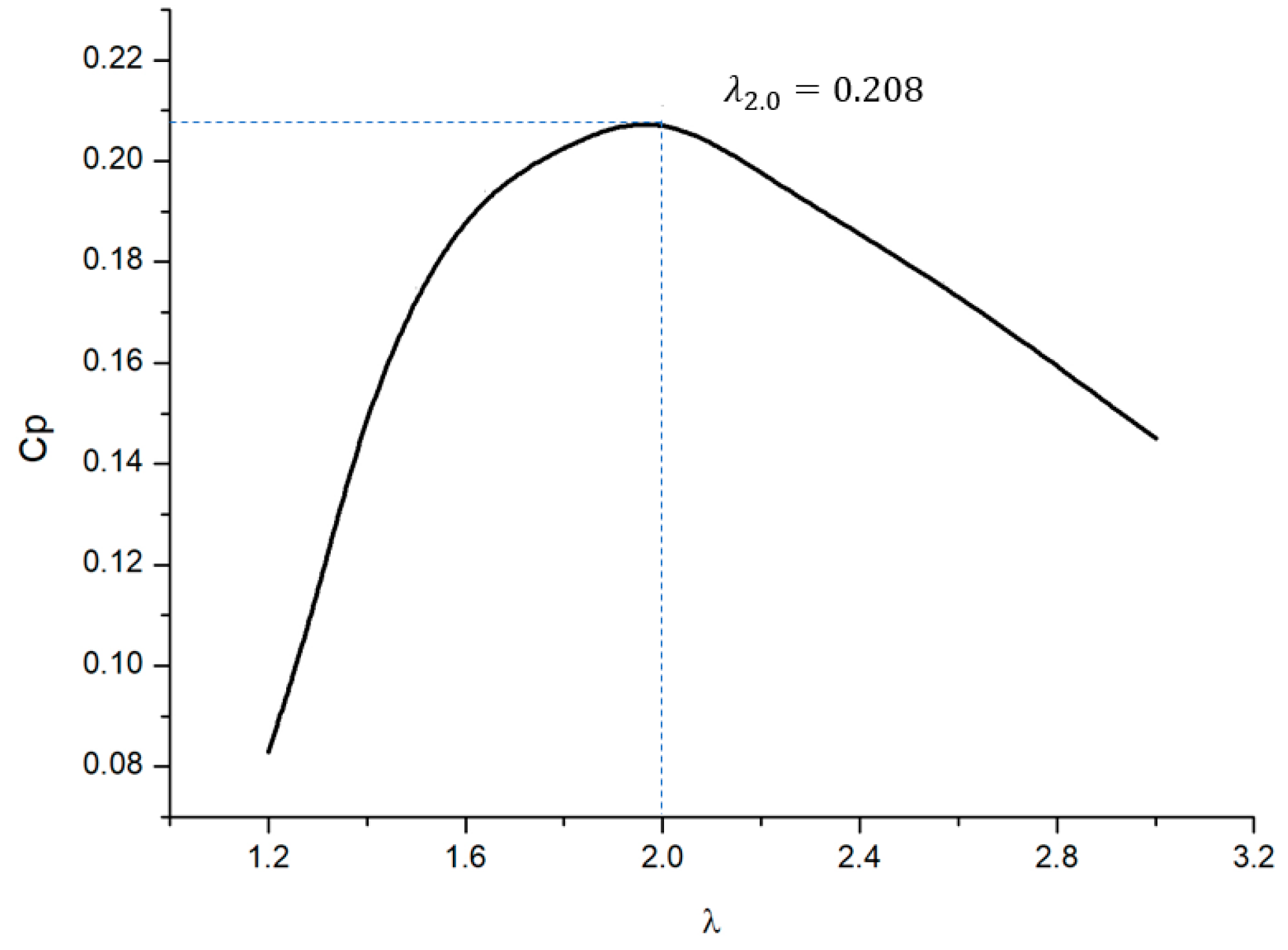
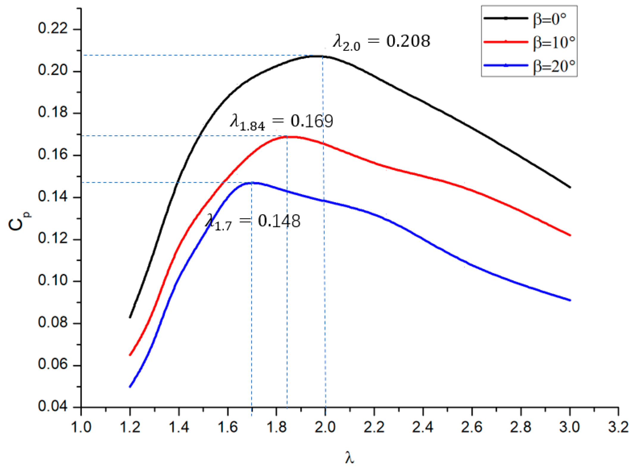
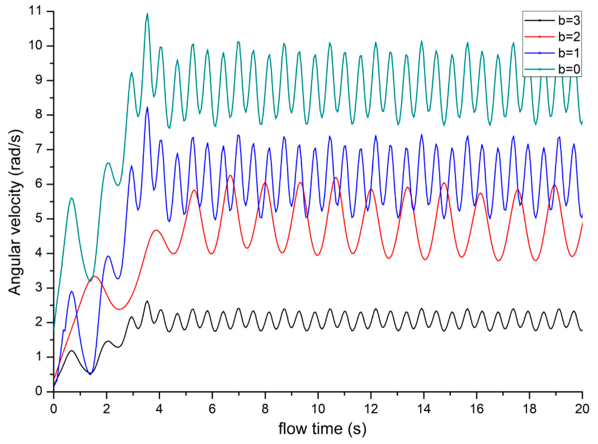
4.2. Energy Utilization Analysis

The curves of the lift L and the resistance D of the turbine can be obtained by numerical calculation. According to the calculation formula of the second part, the resulting curve of the total hydrodynamic torque and the load moment can be obtained. Figure 10 shows the results of flow velocity V = 0.6 m/s. Since the dynamic characteristics of the system are periodic, the integral of inertia of the right side of the motion balance Equation (13) should be zero within one revolution,

$${\int }_{0^{°}}^{{360}^{°}}J\frac{d\omega }{dt}d\theta =0$$

(18)

At this point, the average hydrodynamic torque acting on the blade during one revolution of the turbine should be equal to the average load moment at the output $\overline{M_F}=\overline{M_A}$.

It can be seen from Figure 10 that after the turbine enters a steady state, both the hydrodynamic torque and the load moment pulsate up and down around 0.08 Nm. The pulsation frequencies of the two are essentially the same. For the severity of pulsation, the hydrodynamic torque is significantly higher than the load torque. The pulsation amplitude of the hydrodynamic torque can reach 0.17 Nm or more, while the load torque is only about 0.11 Nm.

The velocity ratio $\lambda =\omega R/V$ and the energy utilization coefficient C_p corresponding to the different velocity ratios are calculated as shown in Figure 11. It can be seen that as the velocity ratio increases, the energy utilization rate first increases and then decreases. Near the speed ratio λ = 2, C_p reaches the maximum value of 0.208.

The relationships between the energy utilization coefficient and velocity ratio when the incoming flow inclination angles are 10° and 20° are as shown in Figure 12. The results show that the energy utilization decreases with the increase of the inclination angle, and the peak inflection point is advanced. The maximum value is 0.169 when the inclination angle is 10° and the corresponding velocity ratio is about 1.8. The maximum value is 0.148 when the inclination angle is 20° and the corresponding velocity ratio is about 1.7.

Considering that the wind turbine already has more mature research results, Figure 13 compares the results of this paper with the empirical curve of the four-blade fan energy utilization coefficient [28,29]. It can be seen from the figure that the numerical results are very close to the empirical curve of the fan. In the future, the energy utilization effect will be further optimized by changing the number and the parameters of the blades.

5. Conclusions

A marine current energy converter for deep-sea profiling floats is proposed in this paper, and the helical involute blade is designed to harness energy from the radial current and the axial relative flow. The blades are analyzed using computational fluid dynamics technique to determine its motion and hydrodynamic performance. This paper not only provides a specific theoretical research basis for the application of ocean energy resources on profiling floats, but also expands the new ideas of ocean energy utilization technologies for different scales and different application environments. The main findings of the present work are summarized as follows.

Through the analysis of fluid structure interaction, the minimum self-starting velocity of the turbine is about 0.3 m/s, the minimum flow velocity during steady operation is 0.6 m/s, and the maximum energy utilization coefficient is 0.208. When the profiling float is inclined by the current, the minimum self-starting flow velocity is 0.43 m/s within 20°, and the energy utilization coefficient is about 0.15. According to China’s existing ocean energy resource data [30], the self-stating requirements of the turbine can be met, thus ensuring the feasibility of this innovative application. By comparing with the empirical curve of the energy utilization coefficient of the fan impeller, the numerical results are also considerable.

In future research, an overall experimental test will be conducted in order to further optimize the structural parameters and ensure the reliability and adaptability of the device, so as to fully prepare for the final engineering application.

References

1. State Key Laboratory of Marine Geology, Tongji University. Seafloor Observation System: An International Review; MGLab: Shanghai, China, 2006. [Google Scholar]
2. IOOS U.S. Integrated Ocean Observing System: A Blueprint for Full Capability; Version 1.0.; IOOS Office: Maryland, MD, USA, 2010.
3. Available online: https://www.marineinsight.com/shipping-news/leadership-2020 (accessed on 2 January 2017).
4. Available online: https://www.westernchannelobservatory.org.uk/ (accessed on 1 January 2017).
5. Available online: http://theory.people.com.cn/n1/2017/1129/c40531-29674382.html (accessed on 29 November 2017).
6. Shaolei, L. The position of the Beidou profile buoy in the global Argo real-time ocean observing network is at stake. Argo Newslett. 2016, 42, 16–18. [Google Scholar]
7. Renqing, L.; Jianping, X. Argo: A successful decade. Basic Sci. China 2009, 4, 15–21. [Google Scholar]
8. Teledyne Webb Research. Variable Bouyancy Profiling Float. U.S. Patent 8,875,645 B1, 4 November 2014. [Google Scholar]
9. Petzrick, E.; Truman, J.; Fargher, H. Profiling From 6000 m with the APEX-Deep Float. Sea Technol. 2014, 55, 27. [Google Scholar]
10. Chiba, S.; Waki, M.; Kornbluh, R.; Pelrine, R. Innovative Power Generators for Energy Harvesting Using Electroactive Polymer Artificial Muscles. SPIE Proc. 2008, 6927. [Google Scholar] [CrossRef]
11. Saupe, F.; Gilloteaux, J.C.; Bozonnet, P.; Creff, Y.; Tona, P. Latching Control Strategies for a Heaving Buoy Wave Energy Generator in a Random Sea. IFAC Proc. Vol. 2014, 47, 7710–7716. [Google Scholar] [CrossRef]
12. Bastien, S.P.; Sepe, R.B.; Grilli, A.R.; Grilli, S.T.; Spaulding, M.L. Ocean wave energy harvesting buoy for sensors. In Proceedings of the 2009 IEEE Energy Conversion Congress and Exposition, San Jose, CA, USA, 20–24 September 2009; pp. 3718–3725. [Google Scholar]
13. Bai, Y.; Du, M.; Zhou, Q.; Jie, M.; He, W. Proceeding of Tidal Current Energy Conversion System. Ocean Dev. Manag. 2016, 33, 57–63. [Google Scholar]
14. Han, S.; Park, J.; Lee, K.; Park, W.; Yi, J. Evaluation of vertical axis turbine characteristics for tidal current power plant based on in situ experiment. Ocean Eng. 2013, 65, 83–89. [Google Scholar] [CrossRef]
15. Liu, H.; Ma, S.; Li, W.; Gu, H.; Lin, Y.; Sun, X. A review on the development of tidal current energy in China. Renew. Sustain. Energy Rev. 2011, 15, 1141–1146. [Google Scholar] [CrossRef]
16. Kamoji, M.A.; Kedare, S.B.; Prabhu, S.V. Performance tests on helical Savonius rotors. Renew. Energy 2009, 34, 521–529. [Google Scholar] [CrossRef]
17. Gorban, A.N.; Asme, A.M.; Gorlov, A.M.; Silantyev, V.M. Limits of the turbine efficiency for free fluid flow. J. Energy Resour. Technol. 2001, 123, 311–317. [Google Scholar] [CrossRef]
18. Gorlov, A.M. Helical turbines for the Gulf Stream: Conceptual approach to design of a large-scale floating power farm. Mar. Technol. 1998, 35, 175–182. [Google Scholar]
19. Ocean Renewable Power Company [EB/OL]. 2014. Available online: http://orpc.co/default.aspx (accessed on 1 January 2018).
20. Zangiabadi, E.; Edmunds, M.; Fairley, I.; Togneri, M.; Williams, A.; Masters, I.; Croft, N. Computational Fluid Dynamics and Visualisation of Coastal Flows in Tidal Channels Supporting Ocean Energy Development. Energies 2015, 8, 5997–6012. [Google Scholar] [CrossRef] [Green Version]
21. Shih, T.; Liou, W.; Shabbir, A.; Yang, Z.; Zhu, J. A new k-ε eddy viscosity model for high Reynolds number turbulent flows. Comput. Fluids 1995, 3, 227–238. [Google Scholar] [CrossRef]
22. Liu, W.; Xiao, Q.; Cheng, F. A bio-inspired study on tidal energy extraction with flexible flapping wings. Bioinspir. Biomim. 2013, 8, 036011. [Google Scholar] [CrossRef] [PubMed]
23. Le, T.Q.; Lee, K.S.; Park, J.S.; Ko, J.H. Flow-driven rotor simulation of vertical axis tidal turbines: A comparison of helical and straight blades. Int. J. Nav. Archit. Ocean Eng. 2014, 6, 257–268. [Google Scholar] [CrossRef]
24. Liu, Z.; Qu, H.; Shi, H. Numerical Study on Self-Starting Performance of Darrieus Vertical Axis Turbine for Tidal Stream Energy Conversion. Energies 2016, 9, 789. [Google Scholar] [CrossRef]
25. Shujie, W.; Xiaoli, Y.; Peng, Y.; Junzhe, T.; Xiancai, S. Numerical simulation and experimental research on performance of horizontal axis tidal turbine. Acta Energ. Sol. Sin. 2018, 39, 1203–1209. [Google Scholar]
26. Galloway, P.W.; Myers, L.E.; Bahaj, A.S. Experimental and numerical results of rotor power and thrust of a tidal turbine perating at yaw and in waves. In Proceedings of the World Renewable Energy Congress 2011, Linkoping, Sweden, 8–13 May 2011. [Google Scholar]
27. Galloway, P.W.; Myers, L.E.; Bahaj, A.S. Quantifying wave and yaw effects on a scale tidal stream turbine. Renew. Energy 2014, 63, 297–307. [Google Scholar] [CrossRef]
28. Available online: http://www.360doc.com/content/14/0107/17/12109864_343364720.shtml (accessed on 7 January 2014).
29. Zhu, J.Y.; Huang, H.L.; Shen, H. Self-starting aerodynamics analysis of vertical axis wind turbine. Adv. Mech. Eng. 2015, 7, 1–12. [Google Scholar] [CrossRef]
30. Chu, Q.; Zhang, X.; Sun, J. Numerical simulation of the tidal current in the East China Sea. Mar. Forecasts 2015, 32, 51–60. [Google Scholar]
Figure 1. (a) The lifting process; (b) the deployment of our profiling float.
Energies 11 02218 g001
Figure 2. (a) 3D drawing of profiling float; and (b) Schematic diagram of the internal profile of the turbine connecting mechanism.
Energies 11 02218 g002
Figure 3. Blade design schematics for (a) Involute blade size determination; (b) Blade axial top view schematic; and (c) Radial blade schematic.
Energies 11 02218 g003
Figure 4. Schematic diagrams of the blade section motion and the force analysis: (a) is driven by axial flow and (b) is driven by radial flow.
Energies 11 02218 g004
Figure 5. Meshing and boundary conditions.
Energies 11 02218 g005
Figure 6. (a) Comparison of the Cp vs. λ response of the experimental results of [26,27] and the simulation results of [25]; (b) comparison of the Cd vs. λ response of the experimental results of [26,27] and the simulation results of [25].
Energies 11 02218 g006
Figure 7. (a)Time-domain curves of angular velocity at different flow velocities; (b) Velocity profile of the cross section of the flow field around the turbine at a certain time; (c) A streamline diagram of the velocity field around the turbine at a certain time.
Energies 11 02218 g007
Figure 8. Time-domain curves of angular velocity at different load factors.
Energies 11 02218 g008
Figure 9. Time history curve of the turbine rotation angular velocity at different inclination angles.
Energies 11 02218 g009
Figure 10. Time history curve of the hydrodynamic moment and the load moment.
Energies 11 02218 g010
Figure 11. The energy utilization coefficient’s variation with the change in the velocity ratio.
Energies 11 02218 g011
Figure 12. The relationship between the energy utilization coefficient and the velocity ratio at different inclination angles.
Energies 11 02218 g012
Figure 13. Comparison of the fan energy utilization coefficient curve with the same number of blades.
Energies 11 02218 g013