Article

Characterization and Prediction of Complex Natural Fractures in the Tight Conglomerate Reservoirs: A Fractal Method

1
College of Geosciences, Northeast Petroleum University, Daqing 163318, China
2
Institute of Geophysics and Geomatics, China University of Geosciences, Wuhan 430074, China
3
State Key Laboratory of Petroleum Resource and Prospecting in China University of Petroleum, Beijing 100083, China
4
Department of Overseas Strategy & Production Planning Research in CNPC International Research Center, Beijing 100083, China
5
Northwest Oil and Gas Field of Southwest Oil & Gas field Company, PetroChina, Jiangyou 621709, China
*
Authors to whom correspondence should be addressed.
Energies 2018, 11(9), 2311; https://doi.org/10.3390/en11092311
Submission received: 28 July 2018 / Revised: 20 August 2018 / Accepted: 31 August 2018 / Published: 2 September 2018

Abstract

:
Using the conventional fracture parameters is difficult to characterize and predict the complex natural fractures in the tight conglomerate reservoirs. In order to quantify the fracture behaviors, a fractal method was presented in this work. Firstly, the characteristics of fractures were depicted, then the fracture fractal dimensions were calculated using the box-counting method, and finally the geological significance of the fractal method was discussed. Three types of fractures were identified, including intra-gravel fractures, gravel edge fractures and trans-gravel fractures. The calculations show that the fracture fractal dimensions distribute between 1.20 and 1.50 with correlation coefficients being above 0.98. The fracture fractal dimension has exponential correlation with the fracture areal density, porosity and permeability and can therefore be used to quantify the fracture intensity. The apertures of micro-fractures are distributed between 10 μm and 100 μm, while the apertures of macro-fractures are distributed between 50 μm and 200 μm. The areal densities of fractures are distributed between 20.0 m·m−2 and 50.0 m·m−2, with an average of 31.42 m·m−2. The cumulative frequency distribution of both fracture apertures and areal densities follow power law distribution. The fracture parameters at different scales can be predicted by extrapolating these power law distributions.

1. Introduction

Natural fractures are one of the key factors affecting the exploration and development of tight oil and gas [1,2,3,4,5]. Many oil and gas fields in the world have been identified as fractured reservoirs [1,4] and the presence of natural fractures significantly increases the porosity and permeability of tight reservoirs [6,7,8,9,10]. Meanwhile, the existence of natural fractures may also facilitate the development and utilization of resources such as fracture water and geothermal resources [11,12,13], cause caprock failures [14,15,16,17] or reservoir leaks in projects (CO2 sequestration, gas storage, nuclear waste disposal, etc.) [18,19], or induce geological disasters [18]. Therefore, quantitative characterization and comprehensive evaluation of natural fractures are very important and urgently needed.
Many studies were devoted to the characteristics, formation mechanisms, characterization methods and evaluations of natural fractures in tight sandstones, carbonatites, volcanics and shales [3,4,5,20,21,22,23,24,25]. Most of the fractures in these rocks are tectonic fractures. These tectonic fractures have long extension wing and stable occurrence, following a uniform orientation, and are often donated as systematic fractures [26,27,28,29,30,31]. However, since great variances exist in gravel diameter, gravel compositions, and interstitial material compositions, the tight conglomerate reservoir often shows a stronger rock mechanical heterogeneity than the other tight rocks [32]. The fractures developed in the tight conglomerates are drastically different in occurrence and geometry, with poor regularity, short extension and extremely complex spatial distributions, which are called non-systematic fractures [33].
At present, the fracture spacing (the vertical distance between two fractures), the linear density (the total number of fractures per unit length), or the areal density (the total length of fractures per unit area) are normally used to evaluate the intensity of systematic fractures [25,34,35,36,37,38]. However, for the complex non-systematic fractures, the spacing and the linear density are difficult to fully describe their development degree and spatial distribution characteristics. The areal density reveals only the trend of the fracture distribution which cannot be used to evaluate the contribution of the fractures to the reservoir. Therefore, it is essential to find a new parameter that can fully characterize the distribution of these complex non-systematic fractures, including the fracture abundance, spatial distribution characteristics.
Fractal geometry provides an effective mathematical tool to describe the irregular, nonlinear, complex, and naturally occurring objects, which covers almost all fields of the earth science [39,40,41,42,43,44,45]. In recent years, some studies showed that the complex morphology and distribution of faults and fractures have clear fractal characteristics, allowing to study and evaluate the fractures using fractal method [8,46,47,48,49,50,51,52]. In this study, fractal characterization and prediction methods were applied to study the complex fracture system of the tight conglomerate reservoirs of the Lower Jurassic Zhenzhuchong Formation in the Jiulongshan gas field, China, and the geological significance of the fractal method in characterizing and predicting fractures was discussed.

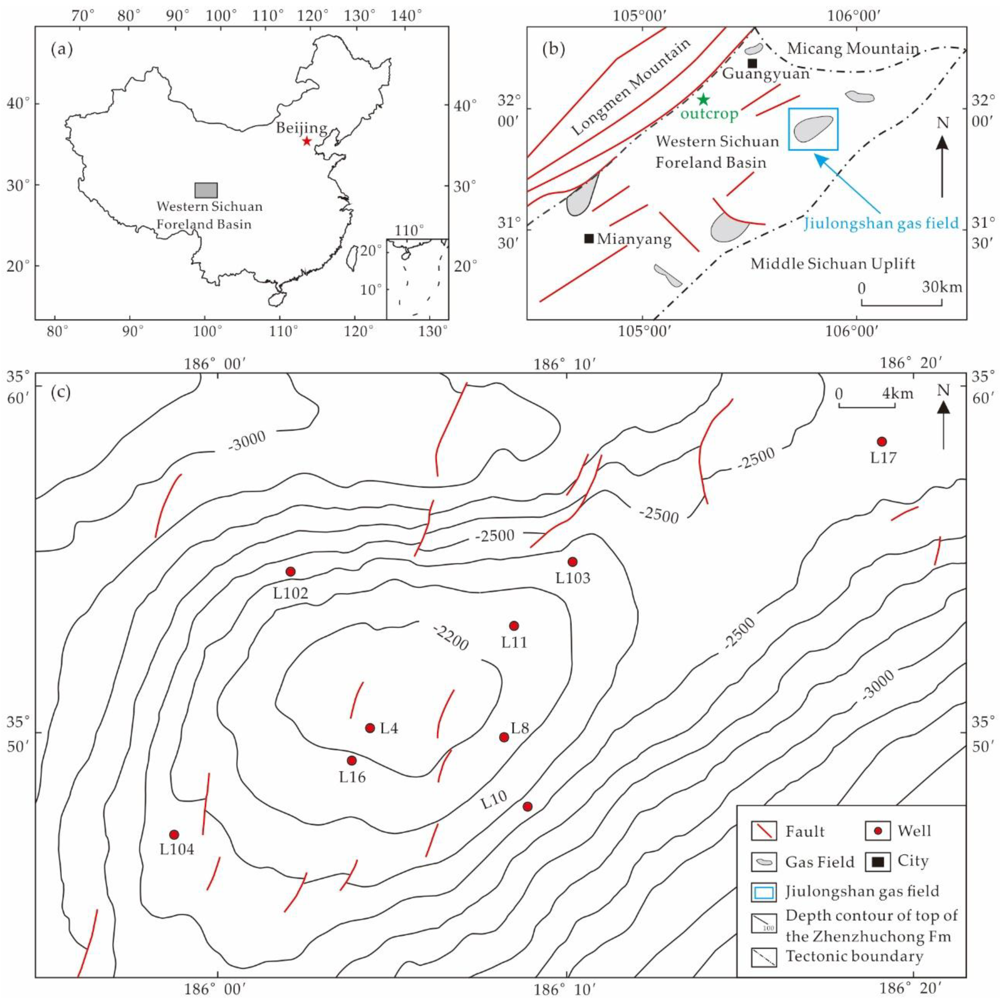
2. Geological Setting

The Jiulongshan gas field is located in the northern part of the Western Sichuan Foreland Basin, China, where the Longmen Mountain thrust belt intersects with the Micang Mountain uplift (Figure 1). The Jiulongshan gas field is a northwest-orientated dome-shaped anticline. Several small reverse faults develop in the study area with throw between 10 m and 100 m [53,54]. The lower Jurassic Zhenzhuchong Formation in this area is a tight conglomerate gas reservoir with formation thickness between 130 m and 210 m and burial depth more than 3000 m. The sedimentary environments are alluvial fan and fan delta front deposits. Reservoir lithology is mainly conglomerate, followed by lithic sandstone. The composition of conglomerate gravels is mainly quartz sandstone (70% to 80%), followed by chert (20% to 30%). The main components of the interstitial material are clastic particles and clay matrix. The sizes of gravels are non-uniform. Even though the gravel sorting is very poor, the degree of roundness is good. The gravel diameters are mainly distributed between 2 mm and 50 mm with a maximum of 80 mm. The pore types of the conglomerate reservoirs are mainly dissolved pores, intergranular pores and fractures.

3. Methodology

Mandelbrot [39] firstly proposed the fractal theory, and defined fractals as shapes whose components are similar to the whole at different scales. The parameter that quantify the self-similarity is the fractal dimension, denoted as D. If the object distribution has fractal features, the number of objects and the measurement scale should follow a power law correlation, as Equation (1):
N(r) = C·r−D,
where N(r) is the number of objects with the specified characteristics; r is the measure scale (cm); C is a constant; D is the fractal dimension.
Take the logarithm at the two sides of Equation (1), as Equation (2):
Log(N(r)) = Log(C) − D·Log(r),
from Equation (2), Log(N(r)) is linear with Log(r), and the slope D of the line is the fractal dimension.
There are many methods existing to calculate fractal dimension, such as the box-counting method, two-point correlation method and mass method, among which the box-counting method is most suitable for the fractal dimension measurement of the spatial distributions of natural fracture systems [42,55,56,57,58]. The generalized steps of the method include:
  • Using a core scanner to obtain high-resolution 360° core images (Figure 2);
  • Covering the image of the entire core with a mesh composed of square grids with side length of r; counting the number N(r) of boxes containing fractures;
  • Gradually changing the side length r of the square grids, and repeatedly counting the corresponding N(r);
  • Taking r as the abscissa and N(r) as the ordinate, using the least-square method to perform regression analysis on the statistical data in the double logarithmic coordinate system (Figure 3).
If the fracture distribution on the core shows fractal features, the Log(N(r)) and Log(r) should follow the linear relationship in Equation (2), and the slope of the regression line is the fracture fractal dimension.
To facilitate intensive analysis, some other parameters were also measured or calculated, such as the fracture aperture, the areal density, the porosity and the permeability. The feeler gauge is used to measure the fracture apertures directly since most of the fractures are opening-mode fractures that do not cut through the cores completely. The feeler gauge used in this study is composed of a set of thin steel sheets with different thicknesses. The thinnest steel sheet is 0.02 mm and the thickest steel sheet is 3 mm. The apertures of micro-fractures were measured with microscope. Fracture areal density is the total length of fractures per unit area, the fracture areal densities of both the cores and the thin sections were characterized. The porosities and permeabilities of 10 full-diameter cores (4 inches in diameter, containing fractures) and 10 core plugs (1 inch in diameter, containing no fracture) were derived using the automated test system for petrophysical parameters at Northeast Petroleum University. Based on the spacing, aperture, length and spatial distribution characteristics of fractures, the fracture porosity and permeability were calculated using the following empirical Equations [60]:
f = 1 S · i = 1 n A i · L i ,
K f = 5.66 × 10 4 · A ¯ 2 · f ,
where ∅f is the fracture porosity (%); S is the core area (m2); Ai is the aperture of the ith fracture (m); Li is the length of the ith fracture (m); Kf is the fracture permeability (mD); and A ¯ is the average fracture aperture (m).

4. Fracture Characterization

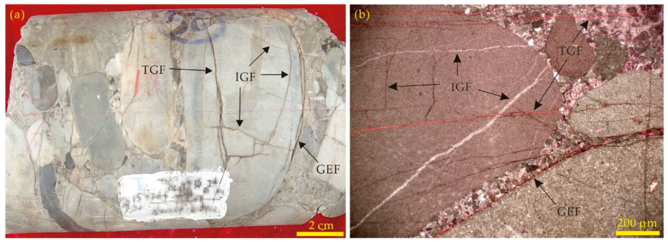
4.1. Fracture Type and Characteristics

According to the spatial distribution characteristics and their relationship with gravels, the fractures in the conglomerate reservoirs can be divided into three types: Intra-gravel fractures (IGF), trans-gravel fractures (TGF) and gravel edge fractures (GEF) (Figure 4).
The intra-gravel fractures are mainly distributed inside the gravels, and they usually have a small extension length and do not cut through the edge of gravels (Figure 4). Such fractures are small in scale but high in density, and their apertures are generally less than 40 μm. The gravel edge fractures are mainly distributed along the edge of the gravels. Hence the surfaces of the gravel edge fractures are either spherical or ellipsoidal, and the fracture traces on cores or thin sections are curves (Figure 5a). This kind of fractures are also small in scale and short in extension, and their apertures are generally less than 20 μm.
The trans-gravel fractures are the major fracture type in the study area (Figure 5b, Figure 6). Most of the trans-gravel fractures are tectonic shear fractures. Compared with the intra-gravel and gravel edge fractures, these trans-gravel fractures are relatively large in scale and long in length. They are not restricted by gravels and usually cut through two or more gravels. According to their dip angles, trans-gravel fractures can be subdivided into fractures with high dip angles and fractures with low dip angles (Figure 6). The high dip angle fractures have long extension on the core, and their height can be as large as 80 cm (Figure 6a). The low dip angle fractures are generally paralleled to each other, and their spacing is between 0.5 cm and 5.0 cm (Figure 6b). Due to the extremely high drilling-encounter ratio, it seems that they are the most important fractures in the cores (Figure 6b). Fractures with both high and low dip angles are very clear on outcrops, they usually appear as conjugate shear fractures (Figure 6c).

4.2. Fracture Parameters

Based on the high-resolution core scanning images, the fractures for 57 intervals from 4 wells were measured using grids with side length of 1 cm, 2 cm, 3 cm, 5 cm, 8 cm, 10 cm and 15 cm, respectively (Figure 2). The numbers of boxes containing fractures were counted and regressions were performed using the least squares method in a log-log coordinate system. Then the fracture fractal dimensions and their corresponding correlation coefficients were calculated. The correlation coefficients of all the cores are above 0.98, indicating that the spatial distribution of fractures in the tight conglomerate has good fractal characteristics (Table 1). The fractal dimensions of core fractures mainly distribute between 1.20 and 1.50, which is reasonable for the fractal range of the two-dimensional object (between 1 to 2) (Figure 7a).
The fracture parameters from cores and thin sections show that the apertures of micro-fractures are mainly distributed between 10 μm and 100 μm, while the apertures of macro-fractures are mainly distributed between 50 μm and 200 μm. The cumulative frequency distribution of both micro- and macro-fractures seems to follow a log-normal distribution (Figure 8). The areal densities of fractures are mainly distributed between 20.0 m·m−2 and 50.0 m·m−2, with an average of 31.42 m·m−2 (Figure 7b). The fracture porosities are mainly distributed between 0.60% and 1.60%, with an average of 1.26% (Figure 7c), and the fracture permeabilities are mainly distributed between 50 mD and 150 mD (Figure 7d).
The core physical property tests show that (Table 2), the porosities of the core plugs are 0.29%–1.60% with an average of 0.97%, and the permeabilities are distributed between 0.0021 mD and 0.0191 mD with an average of 0.0089 mD. The porosity and permeability of the full-diameter cores are significantly larger than those of the core plugs. The porosities of full-diameter cores are distributed between 2.61% and 4.05% with an average of 3.52%. The vertical permeabilities of the full-diameter core are between 0.007 mD and 0.6730 mD with an average of 0.2586 mD, while the horizontal permeabilities are between 3.17 mD and 214.50 mD with an average of 77.7 mD.

5. Discussion

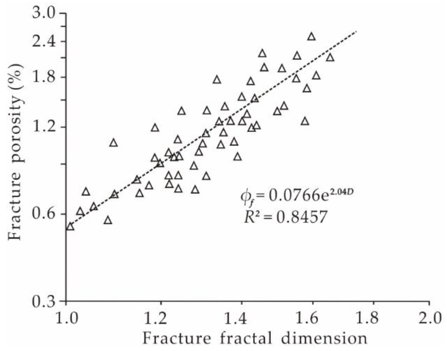
5.1. Geological Significance of Fracture Fractal Dimension

The number of boxes containing fractures has a linear relationship (power law distribution) with the grid side length in double logarithmic coordinate system with correlation coefficients larger than 0.98, demonstrating that the development degree of the fractures in the reservoir follows good fractal features. Therefore, it is reasonable to quantify the development degree and distribution of reservoir fractures using the fractal D value. For example, the fracture fractal dimension D (D = 1.65) of core B is greater than the fracture fractal dimension (D = 1.37) of core A in Figure 2, which means that the fracture in core B is more complex than the fractures in core A. This conclusion is in accordance with the observation, indicating that the fractal dimension D is suitable in characterizing the development degree of these complex fractures. Figure 9 shows that the fracture areal density has an exponential relationship with fracture fractal dimension with a correlation coefficient of 0.8694, indicating that the fracture fractal dimension is a good indicator for the fracture areal density. In addition, the two cores with same fracture areal density have different fracture fractal dimension D. The fracture fractal dimension obtained by the box-counting method also reflects the centralization degree of the fracture distribution of the core specimens [40,42]. The denser the fracture distribution is, the greater the fracture fractal dimension is; vice versa. This indicates that the spatial geometry and complexity of fractures are affecting the fracture fractal dimension.
The fracture fractal dimension is also related to the porosity and permeability of fractures (Figure 10 and Figure 11). Both the porosity and the permeability of fractures show exponential relationships with the fracture dimension with the correlation coefficients of 0.8457 and 0.7718, respectively in this case study. This result shows that the fracture fractal dimension is not limited to characterizing the fracture development degree and the spatial distribution complexity of fractures, but also a good indicator of the porosity and permeability of fractures, improving the understandings of the contributions of fractures to the tight reservoirs [59].

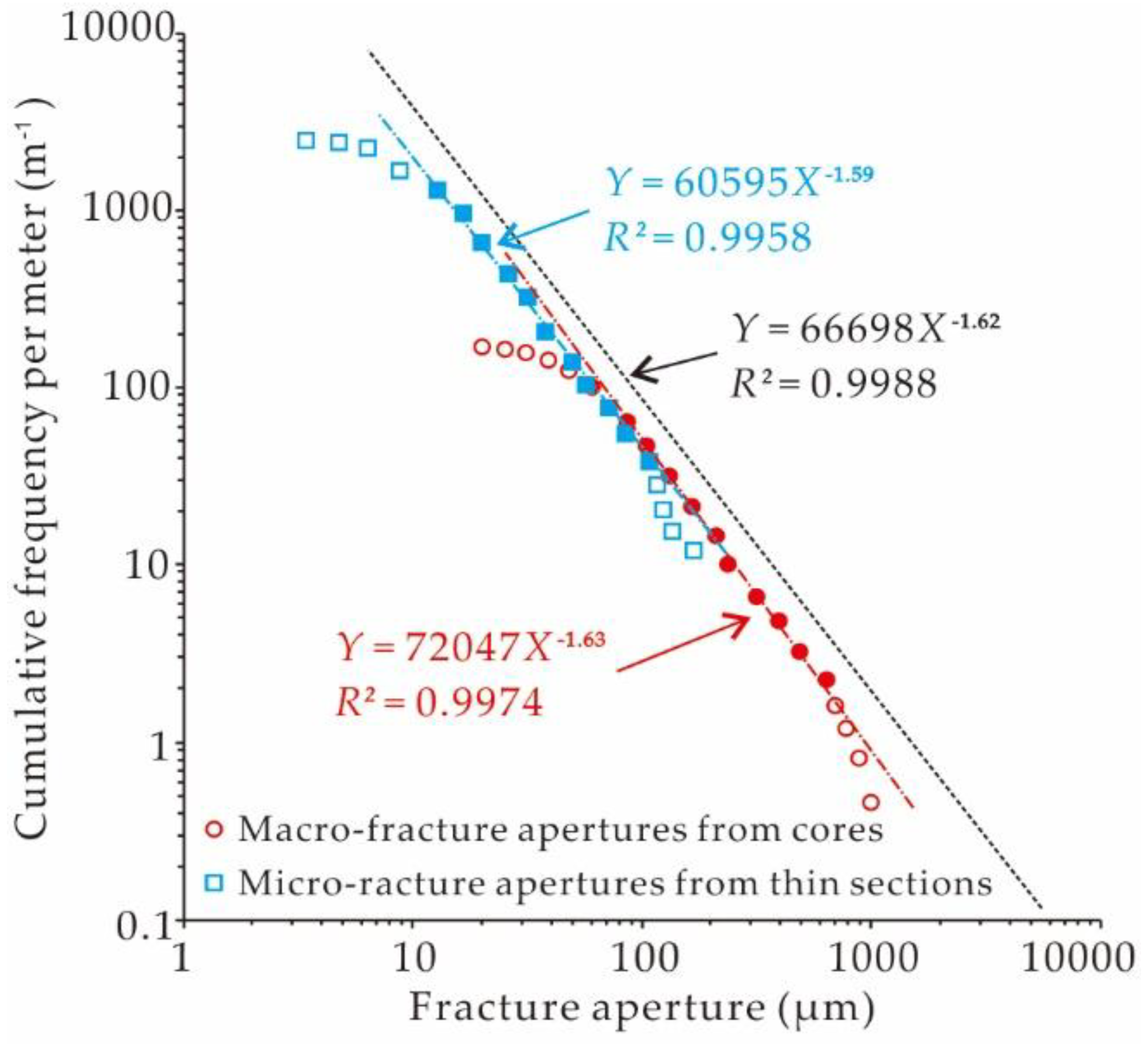
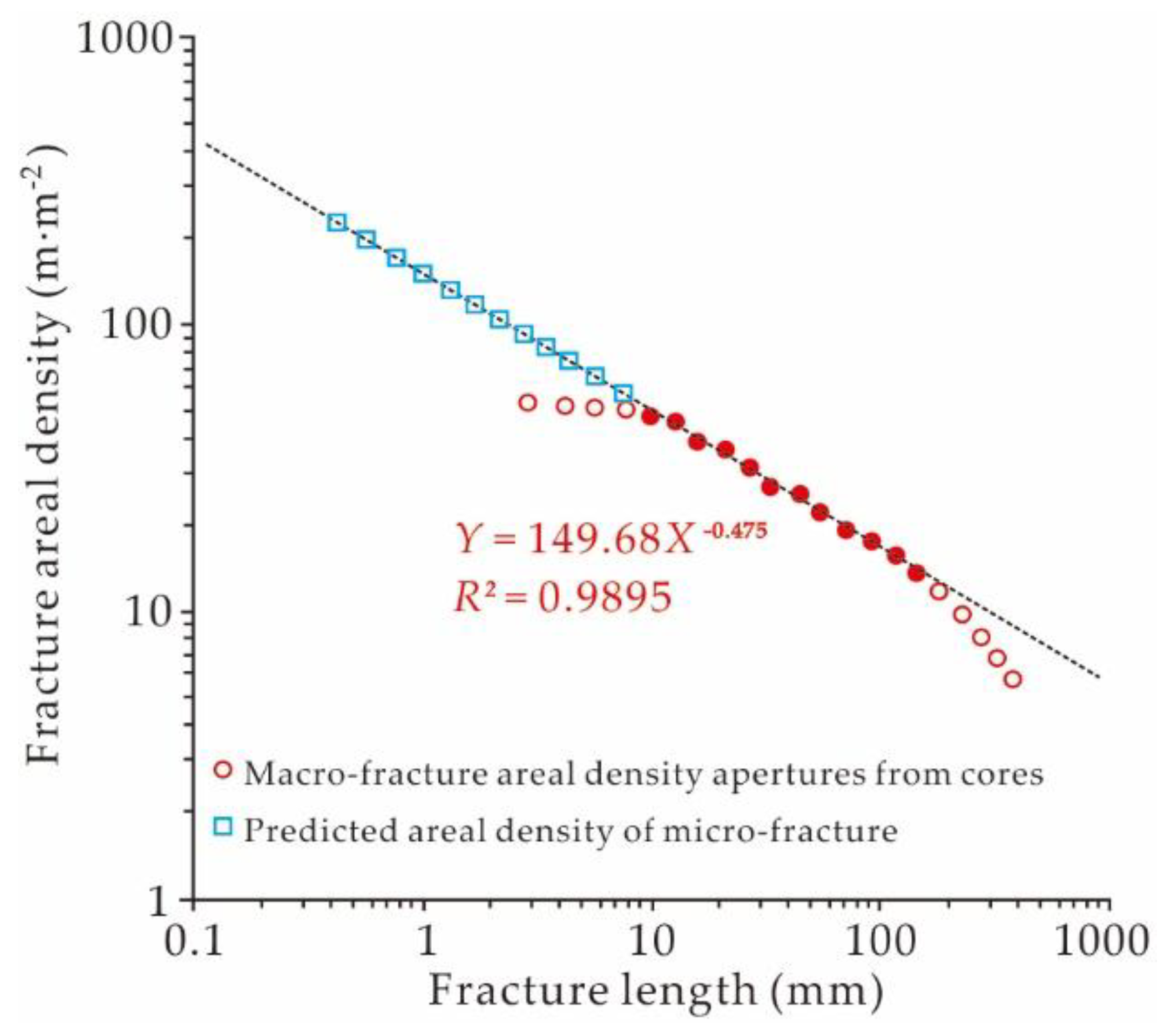
5.2. Power-Law Distribution of Fracture Parameters and Fracture Prediction

The cumulative frequency distribution of fracture parameters (e.g., aperture, areal density, etc.) shows fractal features, providing a theoretical foundation for fracture prediction at different scales [48,50,61,62,63]. Although the cumulative frequency distribution of fracture apertures seems to follow log-normal distribution at a single-observation scale (core scale or thin section scale), after integrating all the aperture data, they are subjected to a uniform power-law distribution, and each scale has almost the same slope (Figure 12). This phenomenon is caused by the truncation and censoring effects [61]. The truncation effect is defined as the phenomenon that the number of the small fractures is underestimated due to the limitation of the observation resolution. The truncation effect causes the upper part of the fracture cumulative frequency distribution curve deviate from the power law distribution. The fractures with large apertures usually cut through the cores making their apertures difficult to be accurately measured. Usually, the measured aperture of these large fractures is lower than the actual value. This is the censoring effect, and due to this effect, the lower part of the fracture cumulative frequency distribution curve will deviate from the power law distribution. Therefore, after eliminating these error data, the number or density of fractures at different scales can be predicted by fine extrapolation of the power law distribution. Using this method, the areal densities of micro-fractures were predicted by extrapolating the power law of cumulative areal density distribution of macro-fractures (Figure 13). Compared to the measured micro-fracture areal density, the errors are less than 5%, which indicates that the prediction results are reliable (Table 3).

5.3. Contribution of Fractures

Since the core plugs are drilled in a way to avoid fractures, while the full-diameter cores are usually drilled through natural fractures, the physical property test results of core plugs represent the physical property of the matrix, and the physical property test results of the full-diameter cores donate the total porosity and permeability of the matrix pores and the natural fractures. Their differences can be roughly regarded as the porosity and permeability of natural fractures. From Table 2, it can be estimated that the porosity of natural fractures is more than 2/3 of the total porosity, and the permeability of natural fractures is 2 to 5 orders of magnitude higher than that of the matrix pores. These observations indicate that natural fractures are the major contributor of the storage space and seepage channel of the tight conglomerate. In addition, the horizontal permeability of the full-diameter cores is much larger than the vertical permeability. This is attributed to the horizontal fractures being dominant in the full-diameter core samples. It also depicts that the natural fractures are the most important seepage channels in the tight conglomerate reservoirs.
The well productivity is also closely related to the development degree of fractures. From Figure 14, the daily gas production is exponentially related to the fracture fractal dimension. The well productivity increases as the fractures develop further. Therefore, the development degree of natural fractures is the most important factor controlling the natural gas enrichment and the capacity of the tight conglomerate reservoir in the Zhenzhuchong Formation.

6. Conclusions

Three types of fractures (IGF, GEF and TGF) exist in the tight conglomerate reservoirs of Zhenzhuchong Formation of Jiulongshan gas field, China, forming a complex fracture network. The fractal dimensions of core fractures mainly distribute between 1.20 and 1.50, which is reasonable for the fractal range of the two-dimensional object (from 1 to 2). The correlation coefficients of all the fracture fractal dimensions are above 0.98, indicating that the spatial distribution of fractures in the tight conglomerate has fractal properties.
The areal densities of fractures are mainly distributed between 20.0 m·m−2 and 50.0 m·m−2, with an average of 31.42 m·m−2. The fracture porosities are mainly distributed between 0.60% and 1.60%, with an average of 1.26%, and the fracture permeabilities are mainly distributed between 50 mD and 150 mD. The fracture fractal dimension has an exponential correlation with the fracture areal density and can therefore be used to quantify the fracture intensity. A good exponential correlation also exists between the fracture fractal dimension and the fracture porosity and permeability, which can reflect their contributions to the physical properties of the tight reservoirs. Therefore, the fracture fractal dimension D is a good comprehensive index as a quantitative parameter to characterize the intensity of the complex fracture system and reflect the contributions of fractures to the tight reservoir.
The apertures of micro-fractures are mainly distributed between 10 μm and 100 μm, and the apertures of macro-fractures are mainly distributed between 50 μm and 200 μm. Although the cumulative frequency distribution of fracture apertures seems to follow log-normal distribution at a single-observation scale (core scale or thin section scale), after integrating all the aperture data, they are subjected to a uniform power-law distribution. The density of micro-fractures was predicted by fine extrapolation of the power law distribution. The errors of predicted results are less than 5%, which indicates that the prediction results are reliable.

Author Contributions

Conceptualization, X.F. and L.Z.; Data curation, P.Z. and B.Z.; Formal analysis, Q.L.; Investigation, B.L.; Methodology, L.G.; Writing—review & editing, L.G., S.G. and W.Y.

Funding

This research was funded by the National Natural Science Foundation of China (grant nos. 41502124 and U1562214), Natural Science Foundation of Heilongjiang Province (grant no. QC2018043), Young Innovative Talents Training Program for Universities in Heilongjiang Province (grant no. UNPYSCT-2018043), China Postdoctoral Science Foundation (grant nos. 2018M631908 and 2015M581424) and Cultivating Fund of Northeast Petroleum University (grant nos. SCXHB201705 and 2017PYQZL-14).

Acknowledgments

The authors thank Yuegang Li, Yong Duan, Hualing Ma, Senqi Pei and Yu Zhang at Northwest Oil and Gas Field of Southwest Oil & Gas field Company, PetroChina for their constructive help.

Conflicts of Interest

The authors declare no conflict of interest.

References

  1. Zeng, L.; Su, H.; Tang, X.; Peng, Y.; Gong, L. Fractured tight sandstone oil and gas reservoirs: A new play type in the Dongpu depression, Bohai Bay Basin, China. AAPG Bull. 2013, 97, 363–377. [Google Scholar] [CrossRef]
  2. Laubach, S.E.; Lamarche, J.; Gauthier, B.D.M.; Dunne, W.M.; Sanderson, D.J. Spatial arrangement of faults and opening-mode fractures. J. Struct. Geol. 2018, 108, 2–15. [Google Scholar] [CrossRef] [Green Version]
  3. Gale, J.F.W.; Laubach, S.E.; Olson, J.E.; Eichhubl, P.; Fall, A. Natural fractures in shale: A review and new observations. AAPG Bull. 2014, 98, 2165–2216. [Google Scholar] [CrossRef]
  4. Nelson, R.A. Geologic analysis of naturally fractured reservoirs; Elsevier: Amsterdam, Netherlands, 2001; Available online: https://www.sciencedirect.com/book/9780884153177/geologic-analysis-of-naturally-fractured-reservoirs (accessed on 17 August 2018).
  5. Bisdom, K.; Gauthier, B.D.M.; Bertotti, G.; Hardebol, N.J. Calibrating discrete fracture-network models with a carbonate three-dimensional outcrop fracture network: Implications for naturally fractured reservoir modeling. AAPG Bull. 2014, 98, 1351–1376. [Google Scholar] [CrossRef]
  6. Ghosh, K.; Mitra, S. Two-dimensional simulation of controls of fracture parameters on fracture connectivity. AAPG Bull. 2009, 93, 1517–1533. [Google Scholar] [CrossRef]
  7. Wang, L.; Zhao, N.; Sima, L.Q.; Meng, F.; Guo, Y. Pore structure characterization of the tight reservoir: Systematic integration of mercury injection and nuclear magnetic resonance. Energy Fuel. 2018, 32, 7471–7484. [Google Scholar] [CrossRef]
  8. Strijker, G.; Bertotti, G.; Luthi, S.M. Multi-scale fracture network analysis from an outcrop analogue: A case study from the Cambro-Ordovician clastic succession in Petra, Jordan. Mar. Petrol. Geol. 2012, 38, 104–116. [Google Scholar] [CrossRef]
  9. Lei, Q.; Wang, X. Tectonic interpretation of the connectivity of a multiscale fracture system in limestone. Geophys. Res. Lett. 2016, 43, 1551–1558. [Google Scholar] [CrossRef] [Green Version]
  10. Larsen, B.; Gudmundsson, A. Linking of fractures in layered rocks: Implications for permeability. Tectonophysics 2010, 492, 108–120. [Google Scholar] [CrossRef]
  11. Magnusdottir, L.; Horne, R.N. Inversion of time-lapse electric potential data to estimate fracture connectivity in geothermal reservoirs. Math. Geosci. 2015, 47, 85–104. [Google Scholar] [CrossRef]
  12. Roques, C.; Bour, O.; Aquilina, L.; Dewandel, B.; Leray, S.; Schroetter, J.; Longuevergne, L.; Le Borgne, T.; Hochreutener, R.; Labasque, T.; et al. Hydrological behavior of a deep sub-vertical fault in crystalline basement and relationships with surrounding reservoirs. J. Hydrol. 2014, 509, 42–54. [Google Scholar] [CrossRef] [Green Version]
  13. Kong, L.; Ostadhassan, M.; Li, C.; Tamimi, N. Pore characterization of 3D-printed gypsum rocks: A comprehensive approach. J. Mater. Sci. 2018, 53, 5063–5078. [Google Scholar] [CrossRef]
  14. Ogata, K.; Senger, K.; Braathen, A.; Tveranger, J. Fracture corridors as seal-bypass systems in siliciclastic reservoir-cap rock successions: Field-based insights from the Jurassic Entrada Formation (SE Utah, USA). J. Struct. Geol. 2014, 66, 162–187. [Google Scholar] [CrossRef]
  15. Petrie, E.S.; Evans, J.P.; Bauer, S.J. Failure of cap-rock seals as determined from mechanical stratigraphy, stress history, and tensile-failure analysis of exhumed analogs. AAPG Bull. 2014, 98, 2365–2389. [Google Scholar] [CrossRef]
  16. Ingram, G.M.; Urai, J.L. Top-seal leakage through faults and fractures: The role of mudrock properties. Geol. Soc. Spec. Publ. 1999, 158, 125–135. [Google Scholar] [CrossRef]
  17. Jin, Z.J. A study on the distribution of oil and gas reservoirs controlled by source-cap rock assemblage in unmodified foreland region of Tarim Basin. Oil Gas Geol. 2014, 35, 763–770. [Google Scholar]
  18. Smith, J.; Durucan, S.; Korre, A.; Shi, J. Carbon dioxide storage risk assessment: Analysis of caprock fracture network connectivity. Int. J. Greenh. Gas Control 2011, 5, 226–240. [Google Scholar] [CrossRef]
  19. Alghalandis, Y.F.; Dowd, P.A.; Xu, C. Connectivity Field: a measure for characterising fracture networks. Math. Geosci. 2015, 47, 63–83. [Google Scholar] [CrossRef]
  20. Gong, L.; Gao, S.; Fu, X.; Chen, S.; Lyu, B.; Yao, J. Fracture characteristics and their effects on hydrocarbon migration and accumulation in tight volcanic reservoirs: A case study of the Xujiaweizi fault depression, Songliao Basin, China. Interpret. J. Sub. 2017, 5, 57–70. [Google Scholar] [CrossRef]
  21. Laubach, S.E.; Fall, A.; Copley, L.; Marrett, R.; Wilkins, S.J. Fracture porosity creation and persistence in a basement-involved Laramide fold, Upper Cretaceous Frontier Formation, Green River Basin, USA. Geol. Mag. 2016, 153, 887–910. [Google Scholar] [CrossRef]
  22. Olson, J.E.; Laubach, S.E.; Eichhubl, P. Estimating natural fracture producibility in tight gas sandstones: coupling diagenesis with geomechanical modeling. Lead. Edge 2010, 29, 1494–1499. [Google Scholar] [CrossRef]
  23. Peacock, D.C.P.; Sanderson, D.J.; Rotevatn, A. Relationships between fractures. J. Struct. Geol. 2018, 106, 41–53. [Google Scholar] [CrossRef]
  24. Sanderson, D.J.; Nixon, C.W. The use of topology in fracture network characterization. J. Struct. Geol. 2015, 72, 55–66. [Google Scholar] [CrossRef]
  25. Lyu, W.Y.; Zeng, L.; Zhang, B.; Miao, F.; Lyu, P.; Dong, S. Influence of natural fractures on gas accumulation in the Upper Triassic tight gas sandstones in the northwestern Sichuan Basin, China. Mar. Petrol. Geol. 2017, 83, 60–72. [Google Scholar] [CrossRef]
  26. Gross, M.R.; Eyal, Y. Throughgoing fractures in layered carbonate rocks. Geol. Soc. Am. Bull. 2007, 119, 1387–1404. [Google Scholar] [CrossRef]
  27. Laubach, S.E.; Olson, J.E.; Gross, M.R. Mechanical and fracture stratigraphy. AAPG Bull. 2009, 93, 1413–1426. [Google Scholar] [CrossRef]
  28. Lyu, W.Y.; Zeng, L.B.; Liu, Z.Q.; Liu, G.P.; Zu, K.W. Fracture responses of conventional logs in tight-oil sandstones: A case study of the Upper Triassic Yanchang Formation in southwest Ordos Basin, China. AAPG Bull. 2016, 100, 1399–1417. [Google Scholar] [CrossRef]
  29. Luo, Q.Y.; Gong, L.; Qu, Y.S.; Zahng, K.H.; Zhang, G.L.; Wang, S.Z. The tight oil potential of the Lucaogou Formation from the southern Junggar Basin, China. Fuel 2018, 234, 858–871. [Google Scholar] [CrossRef]
  30. Zeng, L.B.; Tang, X.M.; Wang, T.C.; Gong, L. The influence of fracture cements in tight Paleogene saline lacustrine carbonate reservoirs, Western Qaidam Basin, Northwest China. AAPG Bull. 2012, 96, 2003–2017. [Google Scholar] [CrossRef]
  31. Finn, M.D.; Gross, M.R.; Eyal, Y.; Draper, G. Kinematics of throughgoing fractures in jointed rocks. Tectonophysics 2003, 376, 151–166. [Google Scholar] [CrossRef]
  32. Gong, L.; Zeng, L.B.; Zhang, B.J.; Zu, K.W.; Yin, H.; Ma, H.L. Control factors for fracture development in tight conglomerate reservoir of Jiulongshan structure. J. China Univ. Petrol. 2012, 36, 6–12. [Google Scholar]
  33. Huang, N.; Jiang, Y.J.; Liu, R.C.; Li, B.; Zhang, Z.Y. A predictive model of permeability for fractal-based rough rock fractures during shear. Fractals 2017, 25, 1750051. [Google Scholar] [CrossRef]
  34. Marrett, R.; Gale, J.F.W.; Gómez, L.A.; Laubach, S.E. Correlation analysis of fracture arrangement in space. J. Struct. Geol. 2018, 108, 16–33. [Google Scholar] [CrossRef]
  35. Casini, G.; Hunt, D.W.; Monsen, E.; Bounaim, A. Fracture characterization and modeling from virtual outcrops. AAPG Bull. 2016, 100, 41–61. [Google Scholar] [CrossRef]
  36. Santos, R.F.V.C.; Miranda, T.S.; Barbosa, J.A.; Gomes, I.F.; Matos, G.C.; Gale, J.F.W.; Neumann, V.H.L.M.; Guimaraes, L.J.N. Characterization of natural fracture systems: Analysis of uncertainty effects in linear scanline results. AAPG Bull. 2015, 99, 2203–2219. [Google Scholar] [CrossRef]
  37. Zeeb, C.; Gomez-Rivas, E.; Bons, P.D.; Blum, P. Evaluation of sampling methods for fracture network characterization using outcrops. AAPG Bull. 2013, 97, 1545–1566. [Google Scholar] [CrossRef]
  38. Procter, A.; Sanderson, D.J. Spatial and layer-controlled variability in fracture networks. J. Struct. Geol. 2018, 108, 52–65. [Google Scholar] [CrossRef]
  39. Mandelbrot, B.B. The fractal geometry of nature; W.H. Freeman and Company: New York, NY, USA, 1982; Available online: https://us.macmillan.com/books/9780716711865 (accessed on 17 August 2018).
  40. Cai, J.C.; Wei, W.; Hu, X.Y.; Liu, R.C.; Wang, J.J. Fractal characterization of dynamic fracture network extension in porous media. Fractals 2017, 25, 1750023. [Google Scholar] [CrossRef]
  41. Cai, J.; Hu, X.; Xiao, B.; Zhou, Y.; Wei, W. Recent developments on fractal-based approaches to nanofluids and nanoparticle aggregation. Int. J. Heat Mass Transf. 2017, 105, 623–637. [Google Scholar] [CrossRef] [Green Version]
  42. Liu, R.; Yu, L.; Jiang, Y.; Wang, Y.; Li, B. Recent developments on relationships between the equivalent permeability and fractal dimension of two-dimensional rock fracture networks. J. Nat. Gas Sci. Eng. 2017, 45, 771–785. [Google Scholar] [CrossRef]
  43. Zhao, P.; Wang, L.; Sun, C.; Cai, C.; Wang, L. Investigation on the pore structure and multifractal characteristics of tight oil reservoirs using NMR measurements: Permian Lucaogou Formation in Jimusaer Sag, Junggar Basin. Mar. Petrol. Geol. 2017, 86, 1067–1081. [Google Scholar] [CrossRef]
  44. Liu, K.Q.; Ostadhassan, M.; Zhou, J.; Gentzis, T.; Rezaee, R. Nanoscale pore structure characterization of the Bakken shale in the USA. Fuel 2017, 209, 567–578. [Google Scholar] [CrossRef]
  45. Zhao, P.; Cai, J.; Huang, Z.; Ostadhassan, M.; Ran, F.Q. Estimating permeability of shale gas reservoirs from porosity and rock compositions. Geophysics 2018, 83, 1–36. [Google Scholar] [CrossRef]
  46. Liu, R.; Li, B.; Jing, H.; Wei, W. Analytical solutions for water–gas flow through 3D rock fracture networks subjected to triaxial stresses. Fractals 2018, 26, 1850053. [Google Scholar] [CrossRef]
  47. Jafari, A.; Babadagli, T. Estimation of equivalent fracture network permeability using fractal and statistical network properties. J. Petrol. Sci. Eng. 2012, 92–93, 110–123. [Google Scholar] [CrossRef]
  48. Johri, M.; Zoback, M.D.; Hennings, P. A scaling law to characterize fault-damage zones at reservoir depths. AAPG Bull. 2014, 98, 2057–2079. [Google Scholar] [CrossRef]
  49. Maerten, L.; Gillespie, P.; Daniel, J. Three-dimensional geomechanical modeling for constraint of subseismic fault simulation. AAPG Bull. 2006, 90, 1337–1358. [Google Scholar] [CrossRef]
  50. Ortega, O.J.; Marrett, R.A.; Loubach, S.E. A scale-independent approach to fracture intensity and average spacing measurement. AAPG Bull. 2006, 90, 193–208. [Google Scholar] [CrossRef]
  51. Zhu, J.; Cheng, Y. Effective permeability of fractal fracture rocks: Significance of turbulent flow and fractal scaling. Int. J. Heat Mass Transf. 2018, 116, 549–556. [Google Scholar] [CrossRef]
  52. Huang, N.; Jiang, Y.J.; Liu, R.C.; Xia, Y.X. Size effect on the permeability and shear induced flow anisotropy of fractal rock fractures. Fractals 2018, 26, 1840001. [Google Scholar] [CrossRef]
  53. Li, Y.; Gong, L.; Zeng, L.; Ma, H.; Yang, H.; Zhang, B.; Zu, K. Characteristics of fractures and their contribution to the deliverability of tight conglomerate reservoirs in the Jiulongshan Structure, Sichuan Basin. Nat. Gas Ind. 2012, 32, 22–26. [Google Scholar]
  54. Pei, S.; Dai, H.; Yang, Y.; Li, Y.; Duan, Y. Evolutionary characteristics of T3x2 reservoir in Jiulongshan Structure, northwest Sichuan Basin. Nat. Gas Ind. 2008, 28, 51–53. [Google Scholar]
  55. Babadagli, T.; Develi, K. On the application of methods used to calculate the fractal dimension of fracture surfaces. Fractals 2001, 9, 105–128. [Google Scholar] [CrossRef]
  56. Klinkenberg, B. A review of methods used to determine the fractal dimension of linear features. Math. Geol. 1994, 26, 23–46. [Google Scholar] [CrossRef]
  57. Walsh, J.J.; Watterson, J. Fractal analysis of fracture patterns using the standard box-counting technique: Valid and invalid methodologies. J. Struct. Geol. 1993, 15, 1509–1512. [Google Scholar] [CrossRef]
  58. Roy, A.; Perfect, E.; Dunne, W.M.; McKay, L.D. Fractal characterization of fracture networks: An improved box-counting technique. J. Geophys. Res. 2007, 112, B12. [Google Scholar] [CrossRef]
  59. Gong, L.; Zeng, L.; Miao, F.; Wang, Z.; Wei, Y.; Li, J.; Zu, K. Application of fractal geometry on the description of complex fracture systems. J. Hunan Univ. Sci. Technol. 2012, 27, 6–10. [Google Scholar]
  60. Mu, L.; Zhao, G.; Tian, Z.; Yuan, R.; Xu, A. Prediction of reservoir fractures; Petroleum Industry Press: Beijing, China, 2009; pp. 111–121. [Google Scholar]
  61. Odling, N.E. Scaling and connectivity of joint systems in sandstones from western Norway. J. Struct. Geol. 1997, 19, 1257–1271. [Google Scholar] [CrossRef]
  62. Gauthier, B.D.M.; Lake, S.D. Probabilistic modeling of faults below the limit of seismic resolution in Pelican Field, North Sea, offshore United Kingdom. AAPG Bull. 1993, 77, 761–777. [Google Scholar]
  63. Hooker, J.N.; Laubach, S.E.; Marrett, R. A universal power-law scaling exponent for fracture apertures in sandstones. Geol. Soc. Am. Bull. 2014, 126, 1340–1362. [Google Scholar] [CrossRef]
Figure 1. Location of the Jiulongshan gas field in the Western Sichuan Foreland Basin, China. (a) Location of the Western Sichuan Foreland Basin; (b) structure outline map of the northern part of Western Sichuan Foreland Basin; (c) depth contour and fault distribution of top of the Zhenzhuchong Formation, Jiulongshan oil field.
Energies 11 02311 g001
Figure 2. Core images, fracture traces and meshes. (a) Image of the surface of core A; (b) fracture traces of core A and the grids for box-counting; (c) image of the surface of core B; (d) fracture traces of core B and the grids for box-counting. The side length of the blue boxes is 1 cm, 2 cm, 3 cm, 5 cm, 8 cm, 10 cm and 15 cm, respectively.
Energies 11 02311 g002
Figure 3. Schematic diagram for the calculation of fracture fractal dimension (modified from [59]). (a) Calculation of fracture fractal dimension for core A; (b) Calculation of fracture fractal dimension for core B.
Energies 11 02311 g003
Figure 4. Fracture types in the tight conglomerates. (a) Well L4, 3164.32 m; (b) Well L102, 3198.35 m. IGF = intra-gravel fracture, TGF = trans-gravel fracture, GEF = Gravel edge fracture.
Energies 11 02311 g004
Figure 5. Gravel edge fracture (GEF) and trans-gravel fractures (TGF) in thin sections. (a) Gravel edge fracture (GEF), Well L104, 3175.05 m; (b) trans-gravel fractures (TGF), Well L16, 3159.34 m.
Energies 11 02311 g005
Figure 6. Trans-gravel fractures in cores and out crop. (a) Trans-gravel fractures with high dip angle in core, Well L102, 3185.75 m; (b) trans-gravel fractures with low dip angle in core, Well L104, 3174.65 m; (c) conjugate fractures in outcrop, see Figure 1 for outcrop location.
Energies 11 02311 g006
Figure 7. Distributions of fracture parameters. (a) Distribution of fracture fractal dimension; (b) distribution of fracture areal density; (c) distribution of fracture porosity; (d) distribution of fracture permeability.
Energies 11 02311 g007
Figure 8. Cumulative frequency plots of micro-fracture apertures (blue squares) and macro-fracture apertures (red circles).
Energies 11 02311 g008
Figure 9. Relationship between fractal dimension and fracture areal density.
Energies 11 02311 g009
Figure 10. Relationship between fractal dimension and fracture porosity.
Energies 11 02311 g010
Figure 11. Relationship between fractal dimension and fracture permeability.
Energies 11 02311 g011
Figure 12. Cumulative plot of micro-fracture apertures (blue squares) and macro-fracture apertures (red circles). The power law distribution of micro-fractures (blue Equation) was obtained by fitting the solid square data, the power law distribution of macro-fractures (red Equation) was obtained by fitting the solid circle data, the power law distribution of all fractures (black Equation) was obtained by fitting the solid square and solid circle data and the best fitting line is slightly offset to the right for clarity of the plot.
Energies 11 02311 g012
Figure 13. Cumulative plot of macro-fracture areal density (red circles) and prediction of micro-fracture areal density (blue square). The Equation was obtained by fitting the solid circle data, the opening squares are predicted areal density of micro-fractures by extrapolating the power law of cumulative areal density distribution of macro-fractures.
Energies 11 02311 g013
Figure 14. Relationship between fracture fractal dimension and well productivity.
Energies 11 02311 g014
Table 1. Fracture parameters (fractal dimension, areal density, porosity and permeability) calculated from cores.
Well NameIntervalFractal DimensionCorrelation CoefficientAreal Density (m·m−2)Porosity (%)Permeability (mD)
Top (m)Bottom (m)
L43069.393069.551.380.991040.291.26133.98
L43069.643069.721.220.989126.590.9938.62
L43069.773069.781.220.988425.850.8374.93
L43069.983070.111.280.990127.871.5181.98
L43070.223070.291.310.992026.580.8290.48
L43070.493070.571.400.990840.540.96106.12
L43070.803070.931.430.989836.801.2288.98
L43071.013071.121.100.991424.980.5932.00
L43071.363071.561.240.990532.810.9574.75
L43071.713071.801.580.989739.291.27138.58
L43071.913072.121.170.991421.300.7680.85
L43072.243072.411.010.989317.950.5039.93
L103080.743080.911.150.987724.220.7152.18
L103101.613101.801.280.992726.990.7467.63
L103101.883102.071.030.992224.190.6234.91
L103102.133102.341.650.993356.491.81245.25
L103102.553102.711.240.989424.770.8382.18
L103102.813102.951.310.989640.641.1579.94
L103103.303103.421.240.992331.861.0994.35
L103103.493103.531.330.987932.421.7790.54
L103103.613103.791.360.990040.621.42143.99
L103103.883103.931.400.987635.681.5458.35
L103104.073104.181.370.987536.021.27120.48
L103104.263104.371.360.989528.561.17166.58
L1023087.203087.341.460.988434.292.18114.94
L1023087.513087.571.350.988730.491.05103.49
L1023087.753087.851.500.988645.501.38139.29
L1023087.943088.081.550.987550.571.78191.51
L1023088.233088.331.040.990324.690.7355.77
L1023088.603088.701.050.988618.000.6955.13
L1023089.013089.171.510.990943.761.93218.89
L1023089.173089.281.100.988026.701.0693.28
L1023089.393089.551.080.991820.010.5852.04
L1033117.233117.381.240.988930.601.11128.42
L1033117.453117.541.430.992447.721.75191.26
L1033117.703117.841.440.990641.501.2490.64
L1033117.993118.051.280.990139.061.2675.31
L1033118.153118.261.390.989547.301.0888.36
L1033118.363118.581.190.992828.911.2179.01
L1033118.673118.821.220.988233.350.7635.99
L1033118.983119.031.410.992443.211.35111.74
L1033119.093119.211.190.989428.880.9560.14
L1033119.303119.401.560.992967.272.14169.61
L1033119.583119.721.150.990924.140.8078.47
L1033119.923120.161.310.991534.790.7959.60
L1033120.323120.501.440.993048.271.5390.03
L1033128.183128.371.520.992339.171.44208.87
L1033128.573128.711.240.990525.291.1148.97
Table 2. Porosities and Permeabilities of full-diameter cores and core plugs.
NumberFull Diameter CoresCore PlugsΦ1/Φ2K1/K3
Φ1 (%)K1 (mD)K2 (mD)Φ2 (%)K3 (mD)
13.90214.500.01450.290.002113.45102,142.86
23.74201.690.00070.640.00845.8424,010.71
33.80166.570.06890.510.00567.4529,744.64
43.125.750.02371.510.01052.07547.62
52.6183.580.01230.930.00962.818706.25
64.053.170.59171.600.01912.53165.97
73.047.250.46281.260.00842.41863.10
83.1921.400.24501.090.00472.934553.19
93.0632.300.49300.890.00793.444088.61
103.0140.400.67300.950.01273.173181.10
Average3.5277.70.25860.970.00894.6117,800.40
Note: Φ1 and Φ2 are the porosities of the full-diameter cores and the core plugs respectively; K1 and K2 are horizontal permeability and vertical permeability of the full-diameter cores respectively; K3 is the permeability of the core plugs.
Table 3. Comparation of the measured and predicted areal density of micro-fractures.
Fracture Length (mm)Fracture Areal DensityAbsolute Error (m·m−2)Relative Error (%)
Measured (m·m−2)Predicted (m·m−2)
1050.3550.14−0.210.42
951.8952.710.821.58
856.0555.74−0.310.55
760.4859.39–1.091.80
662.3663.911.552.48
567.0769.692.623.90

