Selection of Calibration Windows for Day-Ahead Electricity Price Forecasting

Abstract

We conduct an extensive empirical study on the selection of calibration windows for day-ahead electricity price forecasting, which involves six year-long datasets from three major power markets and four autoregressive expert models fitted either to raw or transformed prices. Since the variability of prediction errors across windows of different lengths and across datasets can be substantial, selecting ex-ante one window is risky. Instead, we argue that averaging forecasts across different calibration windows is a robust alternative and introduce a new, well-performing weighting scheme for averaging these forecasts.

1. Introduction

Over the last three decades the electricity price forecasting (EPF) literature has focused on selecting explanatory variables and developing better performing statistical or computational intelligence models [1]. However, somewhat surprisingly, it has almost completely ignored the problem of finding the optimal length of the calibration window. Instead, the typical approach has been to select ad-hoc a ‘long enough’ window, e.g., 10–13 days [2,3], 4 weeks [4], 7 weeks (47–50 days) [5,6,7,8], 10 weeks [4], 9 months [1,9,10,11,12], 10 months [13], one year (360–365 days) [8,14,15,16,17,18,19], 1.5 years (44 weeks) [20,21], two years (728–730 days) [22,23,24,25,26,27] or four years [28]. To our best knowledge, only two very recent papers tackle in a systematic way this important, but apparently overlooked problem in EPF [29,30].

Fezzi and Mosetti [29] propose a simple, two-step approach that uses the first step to determine the optimal window length (ranging from only a few to 350 days) for each model and the second step to compare forecasting capabilities across models. They argue that improvements over selecting ex-ante one window of ‘typical’ size are significant for the considered datasets from the Nordic and Italian markets. Hubicka et al. [30] go one step further and propose a novel concept in energy forecasting that combines day-ahead predictions across different calibration windows (ranging from 28 to 728 days). Using data from the Global Energy Forecasting Competition 2014 [31], they show that this kind of averaging yields better results than selecting ex-ante only one ‘optimal’ window length. In this paper, we extend their analysis to other datasets, predictive models with more explanatory variables, transformed price and consumption/load series and—most importantly—introduce a new, well-performing weighting scheme for averaging forecasts.

The remainder of the paper is structured as follows. In Section 2 we introduce the methodology. First, the preliminaries including variance stabilization via the area hyperbolic sine transformation (Section 2.1). Next, the expert autoregressive models with (i.e., ARX) and without (i.e., AR) exogenous variables that are used to compute the day-ahead price forecasts (Section 2.2). Then, the three distinct datasets from three major power markets with 2.5–3 year long out-of-sample test periods (Section 2.3) and the rolling window framework we apply (Section 2.4). Finally, a novel weighting scheme for averaging forecasts across calibration windows (Section 2.5). In Section 3 we evaluate the obtained results in terms of the classical error measure for point forecasts (i.e., the mean absolute error , MAE) and the Giacomini and White [32] test for conditional predictive ability (CPA) to determine significant differences in forecasting accuracy. Finally, in Section 4 we wrap up the results and conclude.

2. Methodology

2.1. Preliminaries

As in many EPF studies, the modeling is implemented here within a ‘multivariate’ framework, which mimics price setting in day-ahead auction markets [27]. We explicitly use a ‘day × hour’, matrix-like structure with $P_{d,h}$ representing the electricity price for day d and hour h. Given the recommendations of Uniejewski et al. [26], we calibrate our models not only to raw prices but also to transformed data, i.e., $X_{d,h}=f\left(P_{d,h}\right)$, where $f(·)$ is an appropriately chosen variance stabilizing transformation (VST). Lower variation and/or less spiky behavior of the input data usually allows the forecasting model to yield more accurate predictions [33].

For electricity markets with only positive prices, the logarithm is the most popular choice for a VST. However, since two out of three datasets analyzed here exhibit negative values, the log-transform is not feasible in our case. Instead, we use the area hyperbolic sine transformation:

$$X_{d,h}=\mathbf{asinh}\left(p_{d,h}\right)\equiv \log \left(p_{d,h}+\sqrt{p_{d,h}^2+1}\right),$$

(1)

where $p_{d,h}=\frac{1}{b}(P_{d,h}-a)$ are ‘normalized’ prices, a is the median of $P_{d,h}$ in the calibration window and b is the sample median absolute deviation (MAD) around the median. The asinh can be used for negative data and its implementation is straightforward. Moreover, it has been found to perform well in several EPF studies [25,27,34]. The inverse transformation is the hyperbolic sine, i.e., $p_{d,h}=\sinh \left(X_{d,h}\right)$. After computing the forecasts, we apply it to obtain the price predictions:

$${\widehat{P}}_{d,h}=b\sinh ({\widehat{X}}_{d,h})+a.$$

(2)

2.2. Expert Models

We consider four autoregressive models, each consisting of 24 submodels—one for each hour of the day. Following [17,22,27], we refer to them as expert models, because they are built on some prior knowledge of experts. All four models come in two variants:

• Benchmark versions that work on raw data. Since the identity $f\left(P_{d,h}\right)\equiv P_{d,h}$ is a special case of a VST, to simplify the notation we refer to it as ID and to the resulting data as ‘ID-transformed’.
• Modified versions that work on asinh-transformed data.

The first model, denoted by ARX1, is a simple autoregressive structure with an exogenous variable (hence X in the name) originally proposed by Misiorek et al. [9] and later used in several EPF studies [13,15,17,18,22,25,35,36,37]. Within this model, the VST-transformed price on day d and hour h is given by:

$$\begin{array}{cc}\hfill X_{d,h}=& {\beta }_{h,0}+\underset{\mathrm{autoregressive} \mathrm{effects}}{\underbrace{{\beta }_{h,1}{X}_{d-1,h}+{\beta }_{h,2}{X}_{d-2,h}+{\beta }_{h,3}{X}_{d-7,h}}}+\underset{\mathrm{non}-\mathrm{linear} \mathrm{effects}}{\underbrace{{\beta }_{h,4}{X}_{d-1,min}}}\hfill \\ & +\underset{\mathrm{load} \mathrm{forecast}}{\underbrace{{\beta }_{h,5}{C}_{d,h}}}+\underset{\mathrm{weekday} \mathrm{dummies}}{\underbrace{{\beta }_{h,6}{D}_{Sat}+{\beta }_{h,7}{D}_{Sun}+{\beta }_{h,8}{D}_{Mon}}}+{\epsilon }_{d,h},\hfill \end{array}$$

(3)

where $X_{d-1,h}$, $X_{d-2,h}$ and $X_{d-7,h}$ account for the autoregressive effects of the previous days (i.e., the same hour yesterday, two days ago and one week ago), $X_{d-1,min}$ is the minimum of the previous day’s 24 h VST-transformed prices and the exogenous variable $C_{d,h}$ refers to the consumption (or load) forecast for day d and hour h (known on day $d-1$ and VST-transformed). The three dummy variables $D_{Sat}$, $D_{Sun}$ and $D_{Mon}$ model the weekly seasonality, and are defined as $D_i=1$ for $d=i$ and zero otherwise. Finally, the ${\epsilon }_{d,h}$’s are assumed to be independent and identically distributed normal variables. The second model, denoted by AR1, is obtained from Equation (3) by setting ${\beta }_{h,5}\equiv 0$, i.e., by discarding the exogenous variable.

The third autoregressive structure is the well-performing $exper{t}_{DoW,nl}$ model of Ziel and Weron [27], only expanded to include one exogenous variable (consumption or load forecast; as in [25]). Within this model, denoted by ARX2, the VST-transformed price on day d and hour h is given by:

$$\begin{array}{cc}\hfill X_{d,h}=& \underset{\mathrm{autoregressive} \mathrm{effects}}{\underbrace{{\beta }_{h,1}{X}_{d-1,h}+{\beta }_{h,2}{X}_{d-2,h}+{\beta }_{h,3}{X}_{d-7,h}}}+\underset{\mathrm{non}-\mathrm{linear} \mathrm{effects}}{\underbrace{{\beta }_{h,4}{X}_{d-1,min}+{\beta }_{h,5}{X}_{d-1,max}}}\hfill \\ & +{\beta }_{h,6}{X}_{d-1,24}+\underset{\mathrm{load} \mathrm{forecast}}{\underbrace{{\beta }_{h,7}{C}_{d,h}}}+\underset{\mathrm{weekday} \mathrm{dummies}}{\underbrace{\sum _{i=1}^7{\beta }_{h,7+i}{D}_i}}+{\epsilon }_{d,h}.\hfill \end{array}$$

(4)

The VST-transformed price for the last load period of the previous day, i.e., $X_{d-1,24}$, is included to take advantage of the fact that prices for early morning hours depend more on the previous day’s price at midnight than on the price for the same hour [22,27,38]. Compared to ARX1 also the maximum of previous day’s VST-transformed prices, i.e., $X_{d-1,max}$, and dummies for the remaining days of the week ($D_4\equiv D_{Tue},D_5\equiv D_{Wed},D_6\equiv D_{Thu},D_7\equiv D_{Fri}$) are included. As there are seven dummies in Equation (4), one of them plays the role of the intercept, hence the missing ${\beta }_{h,0}$ term. The fourth model, denoted by AR2, is obtained from Equation (4) by setting ${\beta }_{h,7}\equiv 0$, i.e., by discarding the exogenous variable.

2.3. Datasets

For the test ground we have chosen three major power markets that differ in geographic location and generation mix:

• Nord Pool (NP; Northern Europe)—a hydro-dominated (over 50% of generation) market exhibiting strong seasonal variations,
• PJM Interconnection (Northeastern United States)—the world’s largest competitive wholesale electricity market with a balanced generation mix (ca. a third of coal, gas and nuclear),
• EPEX Germany and Austria (Central Europe)—a developed market with a rapidly growing share of renewables (wind, solar and biomass; currently over 33% of generation) and pronounced negative prices; the latter are natural in electricity trading—since plant flexibility is limited and costly, incurring a negative price for a few hours can actually be economically optimal [34,39].

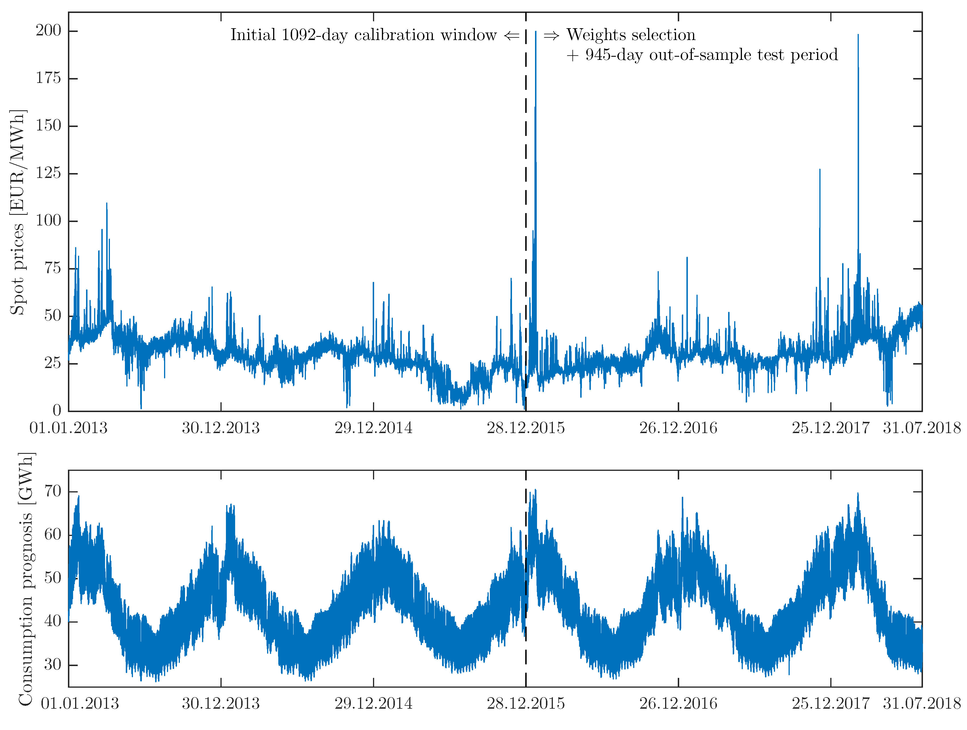
The first dataset comprises two time series at hourly resolution: Nord Pool system prices and day-ahead consumption prognosis for four Nordic countries (Denmark, Finland, Norway and Sweden) from the period 1 January 2013 to 31 July 2018. The time series plotted in Figure 1 were constructed using publicly available data (source: https://www.nordpoolgroup.com/historical-market-data/) and preprocessed to account for missing values and changes to/from the daylight saving time, analogously as in Weron [37]. The missing data values (corresponding to the changes to the daylight saving/summer time and eight hourly consumption figures for Norway) were substituted by the arithmetic average of the neighboring values. The ‘doubled’ values (corresponding to the changes from the daylight saving/summer time) were substituted by the arithmetic average of the two values for the ‘doubled’ hour. The ARX1 and ARX2 models (for both VSTs) were calibrated to the Nord Pool dataset.

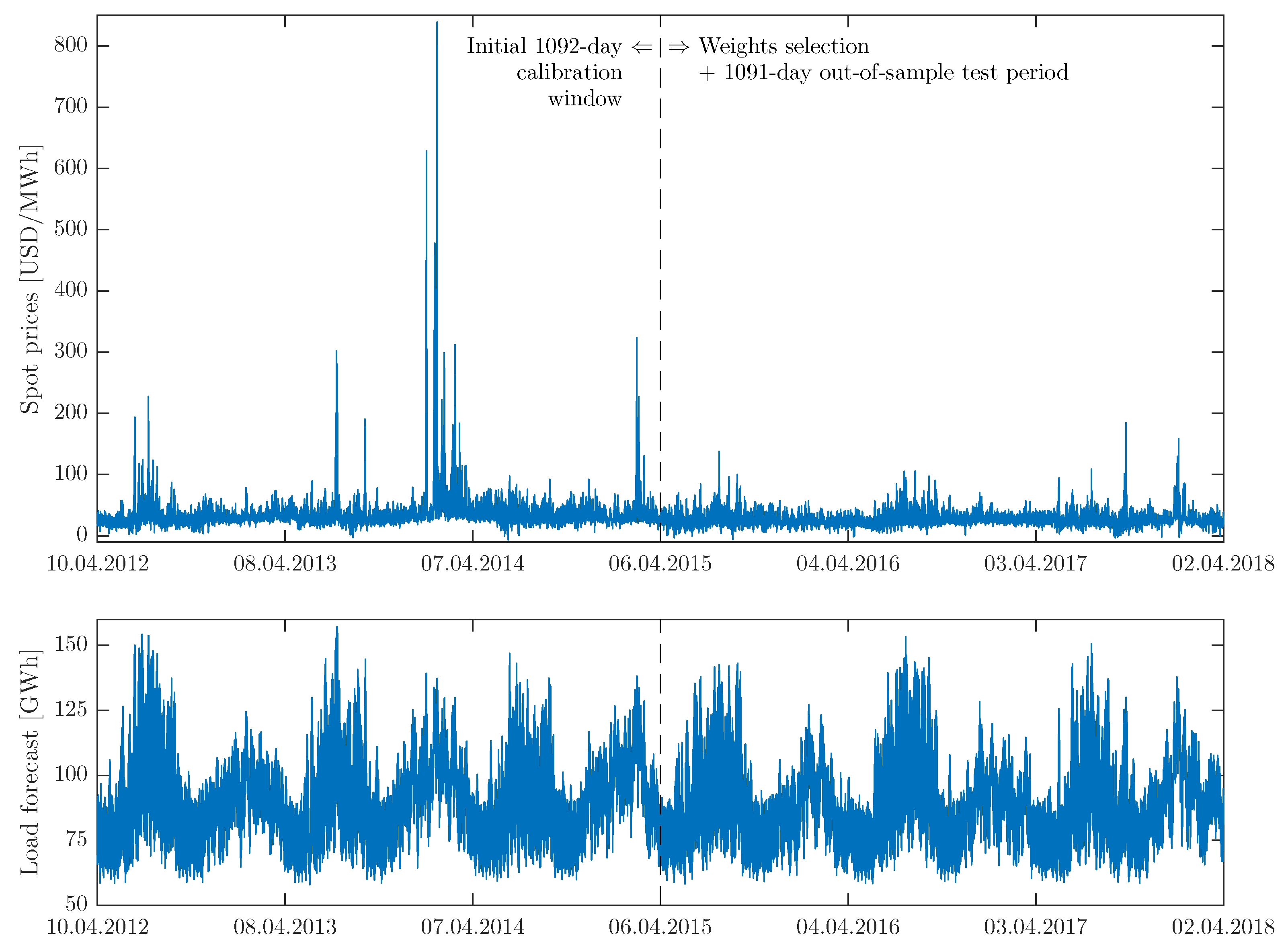
The second dataset also comprises two time series at hourly resolution: prices and day-ahead load forecasts for the Commonwealth Edison (COMED) zone in the PJM market from the period 10 April 2012 to 2 April 2018, see Figure 2. The time series were constructed using publicly available data (source: https://dataminer.pjm.com) and preprocessed to account for missing values and changes to/from the daylight saving time, analogously as the Nord Pool dataset. Note, that although the electricity price units are similar in Figure 1 and Figure 2 (EUR/MWh vs. USD/MWh), the scales on the y-axis are different because of the much more volatile behavior of the PJM market, particularly in early 2014. All four models introduced in Section 2.2 were calibrated to the PJM dataset, resulting in eight different price forecasts for each calibration window: four models × two VSTs.

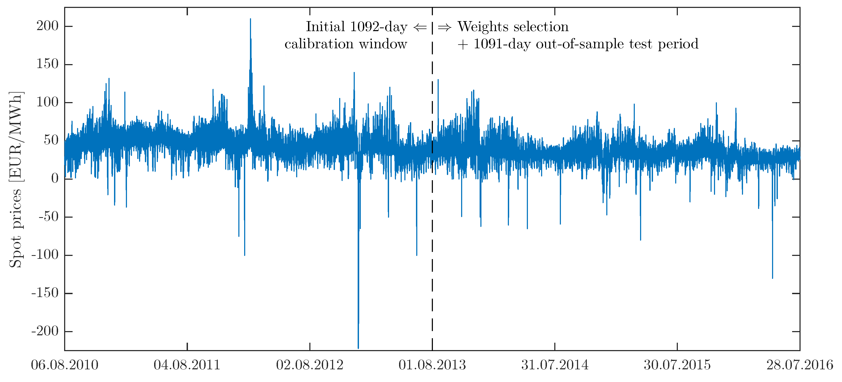
The third dataset comprises hourly prices from the EPEX market for Germany and Austria in the period 6 August 2010–28 July 2016, see Figure 3, that has been used in two recent EPF studies [26,27]. Note, that unlike the Nord Pool and PJM datasets, it does not include an exogenous variable. Consequently, only the ‘pure-price’ AR1 and AR2 models (for both VSTs) were calibrated to the EPEX dataset.

2.4. The Rolling Window Scheme

All three datasets are long enough to comprehensively evaluate day-ahead price predictions: the PJM and EPEX time series span 6 years (2184 days), while the more recent Nord Pool series are 5 months shorter (2038 days). Since the longest calibration window we consider is 3 years long, the out-of-sample test periods span 2.5–3 years, see Figure 1, Figure 2 and Figure 3.

Like the majority of EPF studies, we consider a rolling window scheme. Initially, the first 1092 ($=3\times 364$) days are used for calibration of the expert models. Since this study is concerned with the optimal choice of the calibration window length, we consider 28- to 1092-day windows. For windows shorter than 1092 days, the calibration sample is left-truncated so that it ends on the same day as the 1092-day window. Then, the WAW weights (see Section 2.5) are selected based on price predictions for the following day, i.e., 29 December 2015 for Nord Pool, 7 April 2015 for PJM and 2 August 2013 for EPEX. The remaining observations constitute the 1091- (for PJM and EPEX) or 945-day (for Nord Pool) out-of-sample test periods. Once the price forecasts are obtained for 30 December 2015 (Nord Pool), 8 April 2015 (PJM) and 3 August 2013 (EPEX), the calibration windows are rolled forward by one day and price forecasts for the 24 h of the next day are computed. This procedure is repeated until the predictions for the last day in the test period are obtained.

2.5. Averaging Forecasts across Calibration Windows

Hubicka et al. [30] have recently proposed a novel concept in energy forecasting and shown that averaging day-ahead EPFs across different calibration windows yields better results than selecting ex-ante only one ‘optimal’ window length. Their idea is inspired by the econometric literature, where some researchers argue that forecasting performance is sensitive to the choice of the calibration window and in the presence of structural breaks (i.e., abrupt and unexpected changes in the underlying process) it may be advisable to combine forecasts based on windows of different lengths [40,41]. The rationale behind this approach is that longer windows allow for more precise estimation of model parameters, but shorter better adapt to changes. Consequently, forecasts obtained from models calibrated over windows of different lengths will address distinct features of the underlying process. A similar concept, but limited to two window lengths (2- and 3-year), has been recently considered in load forecasting [42,43].

Here, we extend the analysis of Hubicka et al. [30] to other datasets, predictive models with more explanatory variables, VST-transformed price and consumption/load series and—most importantly—a new weighting scheme for averaging forecasts. As discussed in Section 2.4, we first compute EPFs for 1065 different calibration window lengths, ranging from 28 to 1092 days; we use Win(T) to denote the forecast for a calibration window of length T days. Obviously, we do not know ex-ante which T leads to the most accurate predictions and—as we will see in Section 3—the variability of forecast errors across the T’s and across the datasets can be substantial. Hence, selecting ex-ante one window length is risky. However, as Hubicka et al. [30] argue, a simple arithmetic average of the Win(T)’s across many T’s is a robust alternative that outperforms many Win(T)’s. We denote such a forecast by AW($\mathcal{T}$), where $\mathcal{T}$ is the set of window lengths used. We use Matlab’s notation for the latter, e.g., $\mathcal{T}=$ (28,728) refers to 28- and 728-day windows, $\mathcal{T}=$ (28:28:728) to 26 windows—28-, 56- ($=2\times 28$), ..., 728-day, and $\mathcal{T}=$ (28:1092) to all 1065 windows ranging from 28 to 1092 days.

While AW(28:1092) is robust, it is not computationally efficient, especially if more CPU-demanding predictive models than regression are used; it involves repeating the estimation exercise over 1000 times and for committee machines of neural networks this can be a cumbersome task [18]. The more ‘sophisticated’ approach is to cherry-pick only several calibration windows and not necessarily the best ones, as the suboptimal forecasts may actually average better. Hubicka et al. [30] recommend AW(28:28:84, 714:7:728) as it leverages accurate predictions for a mix of short- and long-term windows with computational efficiency and is not significantly outperformed by any other window set in their study. Since we consider calibration windows of up to three years, in Section 3 we will also evaluate AW($\mathcal{T}$)’s for $\mathcal{T}$’s including longer than 2-year windows.

Let us now extend the AW($\mathcal{T}$) concept and introduce a new, non-uniform weighting scheme for averaging forecasts; we denote the resulting price predictions by WAW($\mathcal{T}$). Inspired by the results of Stock and Watson [44] in a macroeconomic and of Nowotarski et al. [13] in an EPF context, we propose to determine weights based on the inverse of the mean absolute error (MAE) for a certain period in the past:

$$w_T=\frac{\frac{1}{{\mathrm{MAE}}_{\tau ,T}}}{{\sum }_{T\in \mathcal{T}}\frac{1}{{\mathrm{MAE}}_{\tau ,T}}},$$

(5)

where $w_T$ is the weight corresponding to a window of length T and ${\mathrm{MAE}}_{\tau ,T}$ is the MAE for a period of $\tau$ days directly preceding the target day and for a calibration window of length T. Using this approach we assign larger weights to windows that have performed well in the past. Note, that as opposed to earlier studies [13,44] which used large $\tau$’s, we suggest to use very short $w_T$-selection periods, so that the weighting scheme catches only the most recent dependencies. In fact, based on a limited simulation study, $\tau =24$ h seems to be close to optimal and is used in this paper. So that, when assigning weights for day d, we look at the performance of each calibration window on the previous day, i.e., $d-1$. However, the concept is more general and can be extended to different $\tau$’s. Finally, the WAW($\mathcal{T}$) weighted forecast for day d and hour h is given by:

$${\widehat{P}}_{d,h}=\sum _{T\in \mathcal{T}}{w}_T{\widehat{P}}_{d,h,T},$$

(6)

where ${\widehat{P}}_{d,h,T}$ is the prediction for day d and hour h obtained for a calibration window of length T.

3. Results

3.1. Evaluation in Terms of MAE

As the main evaluation criterion we consider the mean absolute error (MAE) for the full out-of-sample test period of $D=1091$ (for PJM and EPEX) or 945 days (for Nord Pool):

$$\mathrm{MAE}=\parallel {\mathcal{E}}_{d,h}{\parallel }_1=\frac{1}{24D}\sum _{d=1}^D\sum _{h=1}^{24}\left|{\mathcal{E}}_{d,h}\right|,$$

(7)

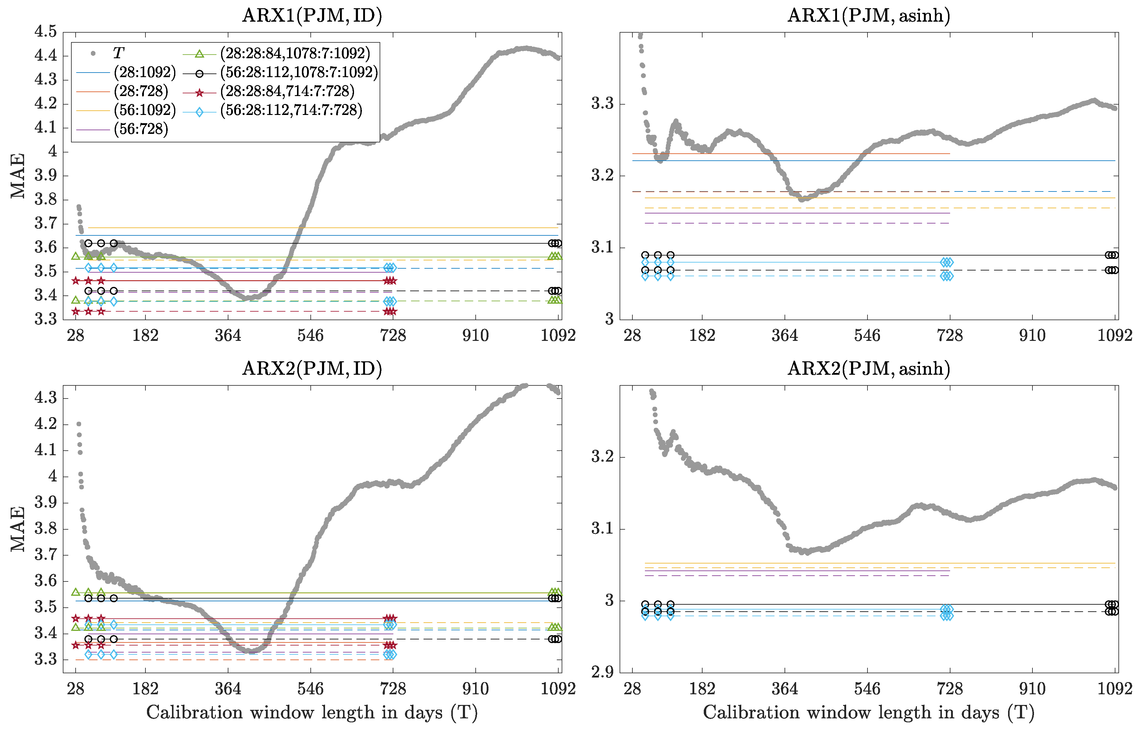
where ${\mathcal{E}}_{d,h}=P_{d,h}-{\widehat{P}}_{d,h}$ is the prediction error for day d and hour h. Results for selected windows (T) and window sets ($\mathcal{T}$) are summarized in

Table 1. Mean absolute errors (MAE) of the ARX1 and ARX2 models fitted to ID- or asinh-transformed Nord Pool (NP) data for selected windows (T) and window sets ($\mathcal{T}$). Relative improvements (%chng) of the Win(T) and WAW($\mathcal{T}$) forecasts with respect to Win(728) are also reported.

	ARX1(NP, ID)			ARX1(NP, asinh)			ARX2(NP, ID)			ARX2(NP, asinh)
Window		Win	%chng		Win	%chng		Win	%chng		Win	%chng
28	2.947		−20.2%	2.713		−15.3%	3.417		−50.7%	3.345		−51.3%
56	2.598		−7.6%	2.255		3.2%	2.423		−16.7%	2.052		−2.4%
364	2.473		−2.7%	2.313		0.7%	2.193		−6.3%	2.052		−2.5%
728	2.407		—	2.329		—	2.058		—	2.002		—
1092	2.333		3.1%	2.258		3.1%	1.981		3.8%	1.960		2.2%
Window Set	AW	WAW	%chng	AW	WAW	%chng	AW	WAW	%chng	AW	WAW	%chng
(28:1092)	2.364	2.348	2.5%	2.227	2.208	5.3%	2.023	2.012	2.2%	1.913	1.906	5.0%
(28:728)	2.401	2.379	1.2%	2.227	2.206	5.4%	2.069	2.055	0.2%	1.921	1.914	4.5%
(56:1092)	2.378	2.362	1.9%	2.241	2.224	4.6%	2.033	2.021	1.8%	1.925	1.917	4.3%
(56:728)	2.422	2.401	0.3%	2.246	2.228	4.4%	2.083	2.067	−0.5%	1.937	1.929	3.7%
(28:28:84, 1078:7:1092)	2.254	2.229	7.7%	2.113	2.091	10.8%	2.000	1.963	4.7%	1.908	1.870	6.9%
(56:28:112, 1078:7:1092)	2.293	2.263	6.2%	2.126	2.108	10.0%	1.992	1.970	4.4%	1.838	1.836	8.7%
(28:28:84, 714:7:728)	2.281	2.253	6.6%	2.140	2.110	9.8%	2.033	2.000	2.9%	1.925	1.889	5.9%
(56:28:112, 714:7:728)	2.323	2.293	4.9%	2.157	2.130	8.9%	2.026	2.006	2.6%	1.854	1.855	7.6%

,

Table 2. Mean absolute errors (MAE) of the ARX1 and ARX2 models fitted to ID- or asinh-transformed PJM data for selected windows (T) and window sets ($\mathcal{T}$). Relative improvements (%chng) of the Win(T) and WAW($\mathcal{T}$) forecasts with respect to Win(728) are also reported. MAEs in excess of ${10}^{10}$ are denoted by ∞; for these values we do not provide %chng.

	ARX1(PJM, ID)			ARX1(PJM, asinh)			ARX2(PJM, ID)			ARX2(PJM, asinh)
Window		Win	%chng		Win	%chng		Win	%chng		Win	%chng
28	3.995		2.0%	68.409		−304.6%	5.141		−25.7%	∞		—
56	3.563		13.5%	3.288		−1.1%	3.691		7.4%	3.365		−7.5%
364	3.433		17.2%	3.196		1.8%	3.383		16.2%	3.093		0.9%
728	4.078		—	3.253		—	3.976		—	3.121		—
1092	4.391		−7.4%	3.294		−1.2%	4.321		−8.3%	3.157		−1.2%
Window Set	AW	WAW	%chng	AW	WAW	%chng	AW	WAW	%chng	AW	WAW	%chng
(28:1092)	3.653	3.515	14.9%	3.221	3.178	2.3%	3.526	3.414	15.2%	∞	∞	—
(28:728)	3.465	3.379	18.8%	3.231	3.178	2.3%	3.367	3.300	18.6%	∞	∞	—
(56:1092)	3.684	3.549	13.9%	3.170	3.156	3.0%	3.555	3.443	14.4%	3.053	3.046	2.4%
(56:728)	3.499	3.415	17.8%	3.148	3.134	3.7%	3.399	3.330	17.7%	3.042	3.035	2.8%
(28:28:84, 1078:7:1092)	3.563	3.379	18.8%	13.811	9.853	−110.8%	3.557	3.422	15.0%	∞	∞	—
(56:28:112, 1078:7:1092)	3.620	3.421	17.6%	3.090	3.069	5.8%	3.536	3.380	16.3%	2.996	2.985	4.4%
(28:28:84, 714:7:728)	3.463	3.335	20.1%	13.801	10.360	−115.8%	3.458	3.356	17.0%	∞	∞	—
(56:28:112, 714:7:728)	3.517	3.377	18.9%	3.080	3.061	6.1%	3.435	3.321	18.0%	2.989	2.980	4.6%

,

Table 3. Mean absolute errors (MAE) of the AR1 and AR2 models fitted to ID- or asinh-transformed PJM data for selected windows (T) and window sets ($\mathcal{T}$). Relative improvements (%chng) of the Win(T) and WAW($\mathcal{T}$) forecasts with respect to Win(728) are also reported. MAEs in excess of ${10}^{10}$ are denoted by ∞; for these values we do not provide %chng.

	AR1(PJM, ID)			AR1(PJM, asinh)			AR2(PJM, ID)			AR2(PJM, asinh)
Window		Win	%chng		Win	%chng		Win	%chng		Win	%chng
28	4.437		−7.2%	135.469		−369.8%	5.319		−25.8%	∞		—
56	3.789		8.6%	3.582		−5.8%	3.887		5.6%	3.560		−10.3%
364	3.549		15.1%	3.310		1.3%	3.503		16.0%	3.182		0.9%
728	4.128		—	3.355		—	4.110		—	3.211		—
1092	4.347		−5.2%	3.373		−0.5%	4.415		−7.2%	3.237		−0.8%
Window Set	AW	WAW	%chng	AW	WAW	%chng	AW	WAW	%chng	AW	WAW	%chng
(28:1092)	3.746	3.658	12.1%	3.423	3.341	0.4%	3.648	3.544	14.8%	∞	∞	—
(28:728)	3.592	3.548	15.1%	3.482	3.369	-0.4%	3.500	3.451	17.5%	∞	∞	—
(56:1092)	3.764	3.677	11.6%	3.300	3.295	1.8%	3.671	3.566	14.2%	3.162	3.158	1.7%
(56:728)	3.608	3.565	14.7%	3.293	3.288	2.0%	3.522	3.472	16.9%	3.158	3.154	1.8%
(28:28:84, 1078:7:1092)	3.762	3.658	12.1%	25.185	13.918	−142.3%	3.732	3.606	13.1%	∞	∞	—
(56:28:112, 1078:7:1092)	3.748	3.641	12.6%	3.291	3.287	2.1%	3.667	3.542	14.9%	3.149	3.146	2.0%
(28:28:84, 714:7:728)	3.704	3.616	13.3%	25.183	14.229	−144.5%	3.652	3.546	14.8%	∞	∞	—
(56:28:112, 714:7:728)	3.688	3.605	13.6%	3.289	3.284	2.1%	3.585	3.490	16.3%	3.145	3.143	2.1%

and

Table 4. Mean absolute errors (MAE) of the AR1 and AR2 models fitted to ID- or asinh-transformed EPEX data for selected windows (T) and window sets ($\mathcal{T}$). Relative improvements (%chng) of the Win(T) and WAW($\mathcal{T}$) forecasts with respect to Win(728) are also reported.

	AR1(EPEX, ID)			AR1(EPEX, asinh)			AR2(EPEX, ID)			AR2(EPEX, asinh)
Window		Win	%chng		Win	%chng		Win	%chng		Win	%chng
28	7.069		−22.7%	6.616		−20.8%	7.591		−46.1%	7.560		−48.6%
56	5.922		−5.0%	5.597		−4.0%	5.386		−11.8%	5.131		−9.8%
364	5.571		1.1%	5.345		0.6%	4.769		0.4%	4.616		0.7%
728	5.633		—	5.375		—	4.787		—	4.650		—
1092	5.711		−1.4%	5.461		−1.6%	4.862		−1.6%	4.742		−2.0%
Window Set	AW	WAW	%chng	AW	WAW	%chng	AW	WAW	%chng	AW	WAW	%chng
(28:1092)	5.506	5.498	2.4%	5.301	5.293	1.5%	4.711	4.712	1.6%	4.588	4.587	1.4%
(28:728)	5.494	5.488	2.6%	5.292	5.286	1.7%	4.710	4.711	1.6%	4.583	4.583	1.4%
(56:1092)	5.516	5.509	2.2%	5.313	5.307	1.3%	4.717	4.717	1.5%	4.594	4.592	1.2%
(56:728)	5.504	5.510	2.4%	5.307	5.302	1.4%	4.714	4.713	1.5%	4.587	4.587	1.4%
(28:28:84, 1078:7:1092)	5.537	5.510	2.2%	5.286	5.266	2.1%	4.885	4.850	−1.3%	4.785	4.729	−1.7%
(56:28:112, 1078:7:1092)	5.484	5.472	2.9%	5.267	5.256	2.2%	4.744	4.746	0.8%	4.611	4.609	0.9%
(28:28:84, 714:7:728)	5.529	5.499	2.4%	5.279	5.257	2.2%	4.874	4.831	−0.9%	4.769	4.708	−1.2%
(56:28:112, 714:7:728)	5.476	5.464	3.0%	5.258	5.250	2.4%	4.734	4.732	1.1%	4.592	4.591	1.3%

and plotted in Figure 4, Figure 5, Figure 6 and Figure 7. Note, that when calibrated to asinh-transformed PJM data MAEs of all expert models tend to explode for short windows. This is particularly visible in the rightmost columns in Figure 5 and Figure 6, i.e., respectively for ARX2 and AR2, where MAEs in excess of ${10}^{10}$ are denoted by ∞. As a robustness check, we have also evaluated the results in terms of the root mean squared error (RMSE) and observed only slight differences, e.g., for the ARX2(PJM, ID) model and calibration window sets containing the shortest windows (i.e., shorter than 2 months) WAW was slightly outperformed by AW averaging. Overall, however, the results were qualitatively very similar and are not reported here.

Although there are three datasets in our study, we essentially have four test cases: (i) ARX-type models for Nord Pool in Table 1 and Figure 4; (ii) ARX-type models for PJM in Table 2 and Figure 5; (iii) AR-type models for PJM in Table 3 and Figure 6; and (iv) AR-type models for EPEX in Table 4 and Figure 7. The following conclusions can be drawn regarding performance across the models and VSTs (for a given window or window set):

• Comparing the two expert model structures, i.e., ARX1 vs. ARX2 and AR1 vs. AR2, we can clearly see that the more parsimonious one is outperformed by the larger one. In two test cases (ARX for Nord Pool and AR for EPEX) this is true irrespective of the VST, i.e., ARX2(NP, ID) and AR2(EPEX, ID) yield more accurate predictions than ARX1(NP, asinh) and AR1(EPEX, asinh), respectively. This result supports the observations made by Ziel and Weron [27] that AR(X)2 is a very competitive expert model and can outperform much richer structures.
• Regarding the two VSTs—ID and asinh—clearly the latter one leads to better forecasts than identity (i.e., fitting models to raw data). This can be seen, for instance, by comparing the levels of gray dotted curves representing Win(T) forecasts in the left and corresponding right panels of Figure 4, Figure 5, Figure 6 and Figure 7. This result provides strong support for using variance stabilizing transformations. Although asinh was not the best VST in the study of Uniejewski et al. [26], it is straightforward to implement, its computational cost is negligible and on average it performs very well. We recommend it for EPF.
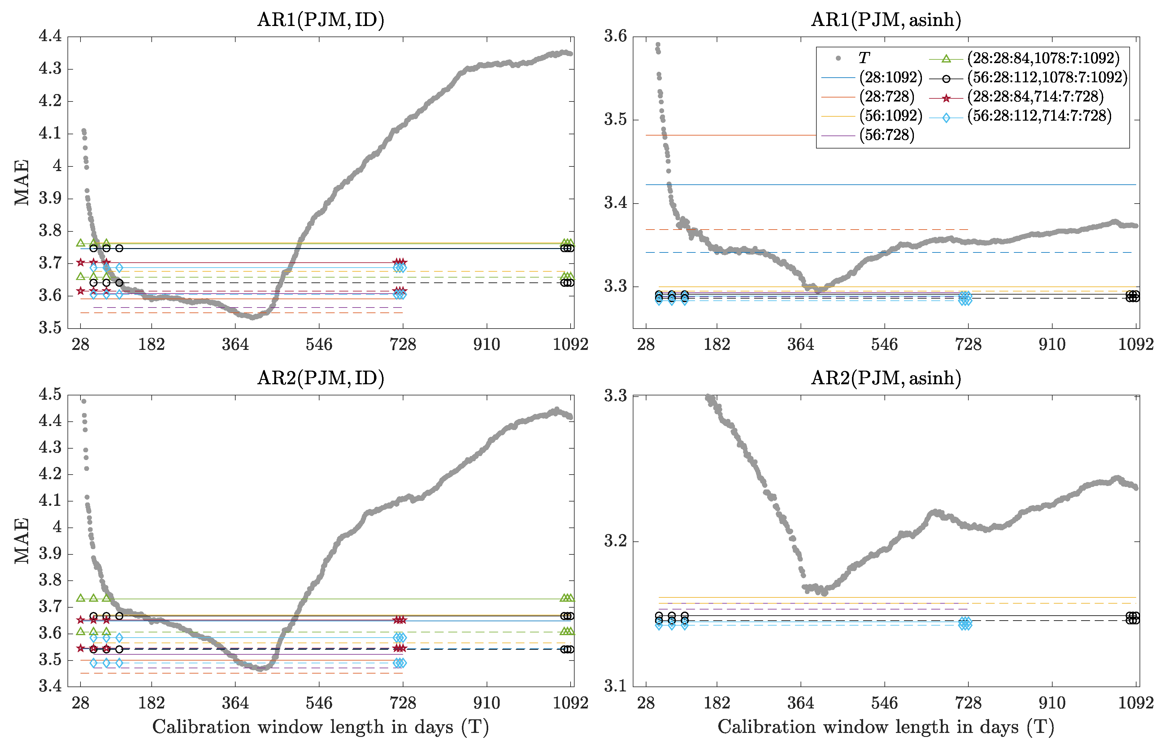
• Autoregressive models with and without the exogenous variable can be compared on the PJM dataset (Table 2 and Figure 5 vs. Table 3 and Figure 6). As is often reported in the EPF literature [1], models with the load forecast as an explanatory variable perform better; in our study by 2–8%, except for a few isolated cases when MAEs of the AR1(PJM, asinh) model exploded.

Now, with respect to the performance of a given model/VST across windows (T) and window sets ($\mathcal{T}$) we can observe that:

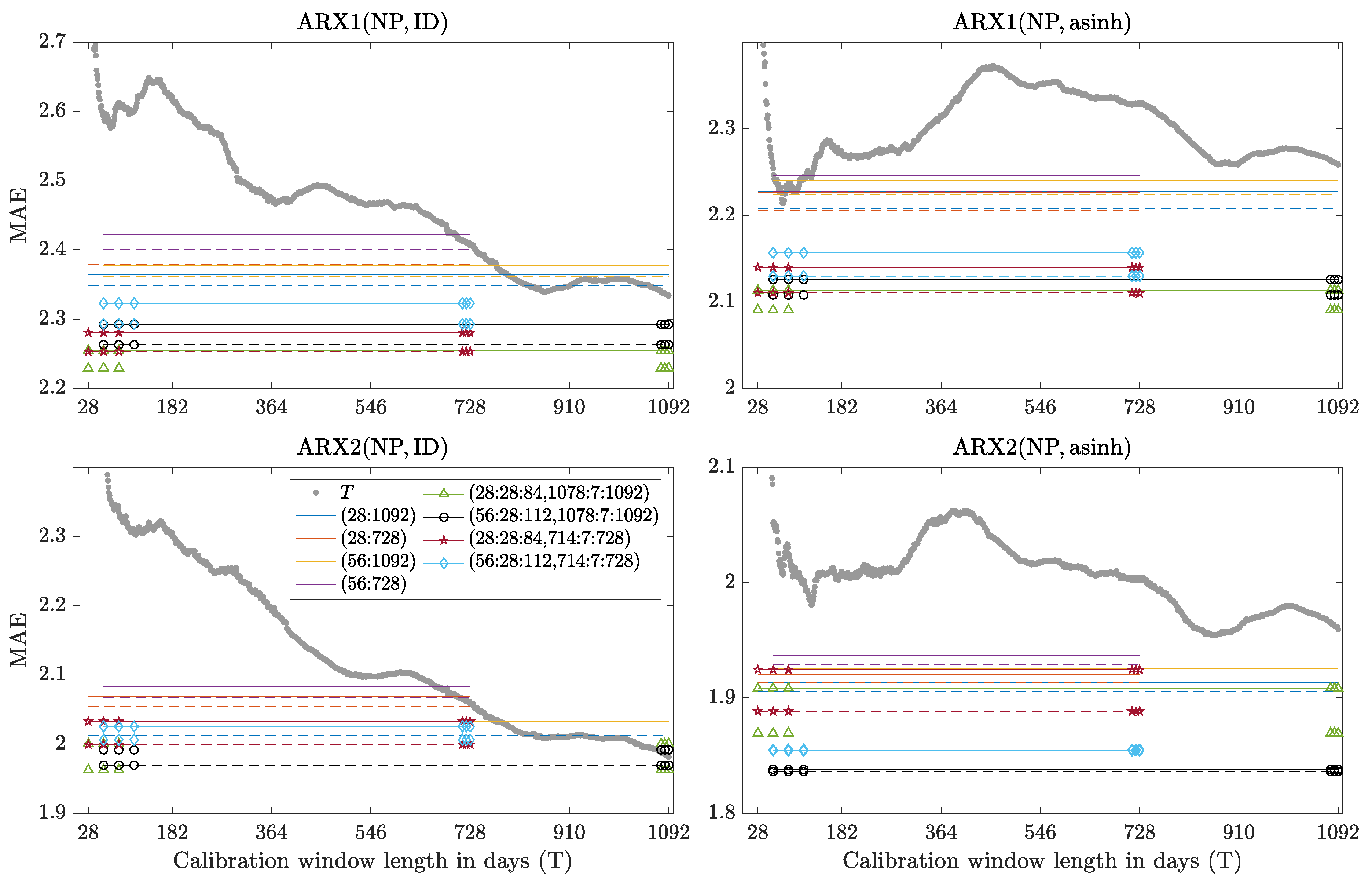
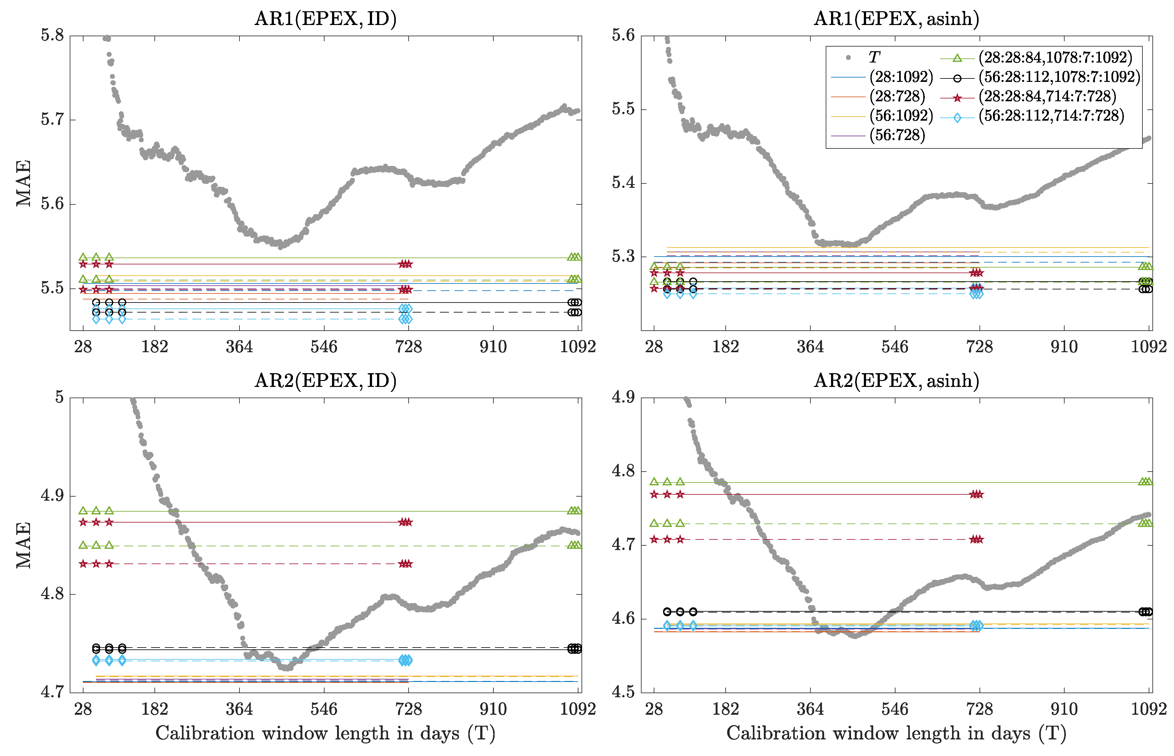
• The behavior of Win(T) as a function of T is very unpredictable. For ARX models calibrated to raw Nord Pool data the MAEs decrease with T and 3-year windows are preferred, see the gray dotted curves in the left panels of Figure 4. However, if the data is asinh-transformed beforehand then the choice of a single window length in not that clear-cut, see the right panels in Figure 4. The picture is completely different for the PJM dataset—now the gray curves have a minimum around 350–450 days and the very long windows are as bad (or even worse) than the very short ones, see Figure 5 and Figure 6. For the EPEX dataset the gray curves also have a minimum around 350–450 days, but now the very long windows are better than the very short ones, see Figure 7. The origins of these minima around 350–450 days are not clear. However, a possible explanation is that time series characteristics changed over time in the PJM and EPEX markets, see the decrease in volatility in Figure 2 and Figure 3, and too long windows include past spikes which are not so pronounced recently.
• Comparing Win(T) with AW and WAW averaging we note in some cases, i.e., for ARX2(NP, asinh), ARX2(PJM, asinh) and AR1(EPEX, *), the latter outperform all Win(T)’s. In many cases averaging outperforms most Win(T)’s, while for AR1(PJM, ID) and AR2(EPEX, asinh) there are a few T’s for which Win(T) is slightly better than any considered average. However, selecting those T’s ex-ante is unlikely. Hence, the presented results support the concept of averaging forecasts across calibration windows.
• Regarding AW and WAW averaging we can observe that the new approach proposed in this paper almost always outperforms the equally weighted scheme of Hubicka et al. [30], i.e., the dashed lines in Figure 4, Figure 5, Figure 6 and Figure 7 are almost always lower than the solid ones of the same color. Moreover, when compared to AW averaging, the WAW scheme decreases the negative impact of a poorly performing calibration window (or a window subset) on the resulting forecast, hence yielding an even more robust outcome.
• An ex-ante choice of $\mathcal{T}$ is not trivial. However, a mix of short- and long-term windows typically outperforms an average across all windows. Recall, that Hubicka et al. [30] recommend AW(28:28:84, 714:7:728) as it leverages accurate predictions with computational efficiency and is not significantly outperformed by any other window set in their study. Our results show that including ca. 3-year windows, e.g., (1078:7:1092), instead of ca. 2-year, e.g., (714:7:728), does not bring visible benefits. However, we suggest to use slightly longer windows at the shorter end, i.e., (56:28:112) instead of (28:28:84), as MAEs for the latter may explode.

Summing up, we recommend using the WAW(56:28:112, 714:7:728) averaging scheme. It is computationally efficient (requires generating only six forecasts for the six calibration windows) and exhibits very good performance across all four autoregressive models, both transformations and all three datasets.

3.2. The CPA Test and Statistical Significance

The obtained MAE values can be used to provide a ranking of models, but do not allow to draw statistically significant conclusions on the outperformance of the forecasts of one model by those of another. Therefore, we use the Giacomini and White [32] test for conditional predictive ability (CPA), which can be regarded as a generalization of the commonly used Diebold and Mariano [45] test for unconditional predictive ability. While both tests can be used for nested and non-nested models—as long as the calibration window does not grow with the sample size [46]—only the CPA test accounts for parameter estimation uncertainty and hence is the preferred option. Here, one statistic for each pair of models is computed based on the 24-dimensional vector of errors for each day:

$${\Delta }_{X,Y,d}=\parallel {\mathcal{E}}_{X,d}\parallel -\parallel {\mathcal{E}}_{Y,d}\parallel ,$$

(8)

where $\parallel {\mathcal{E}}_{Z,d}\parallel ={\sum }_{h=1}^{24}\left|{\mathcal{E}}_{d,h}\right|$ for model Z; by ‘model Z’ we mean here one of the four autoregressive structures defined in Section 2.2 calibrated either on a window of a certain length, i.e., Win(T), or a combined forecast one of the four autoregressive models for a set of windows, i.e., AW($\mathcal{T}$) or WAW($\mathcal{T}$). For each model pair and each dataset we compute the p-value of the CPA test [32] with null $H_0:\varphi =0$ in the regression:

$${\Delta }_{X,Y,d}={\varphi }^{\prime }{\mathbb{X}}_{d-1}+{\epsilon }_d,$$

(9)

where ${\mathbb{X}}_{d-1}$ contains elements from the information set on day $d-1$, i.e., a constant and lags of ${\Delta }_{X,Y,d}$; note, that also the parameters of each of the two models are estimated using data up to day $d-1$.

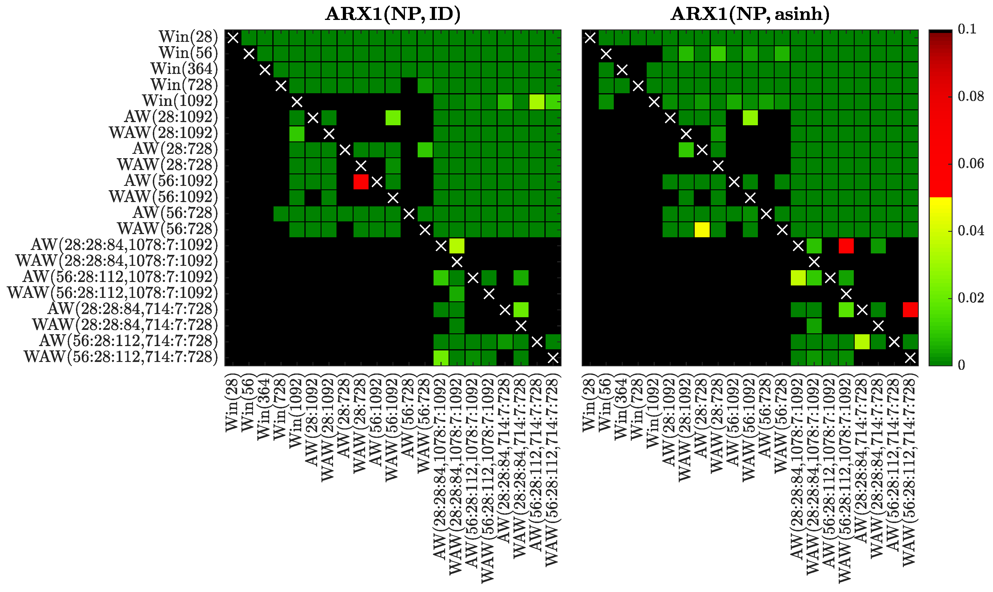
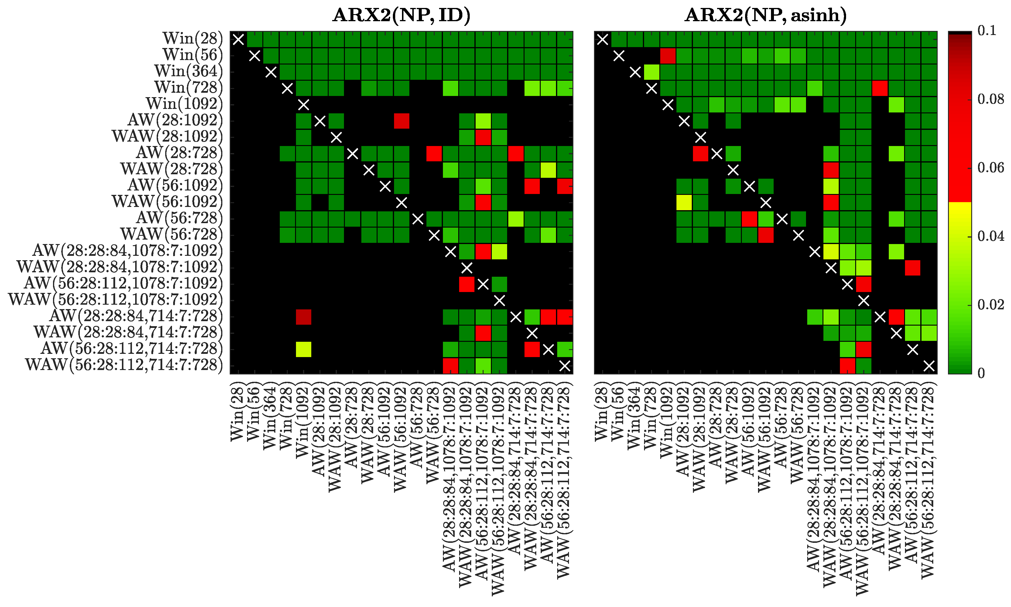
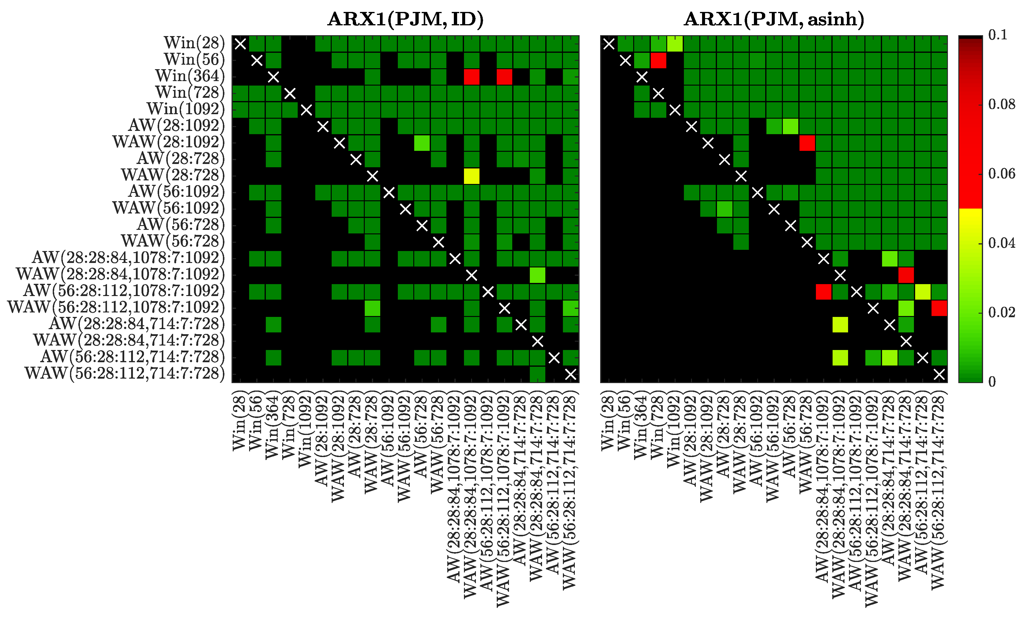
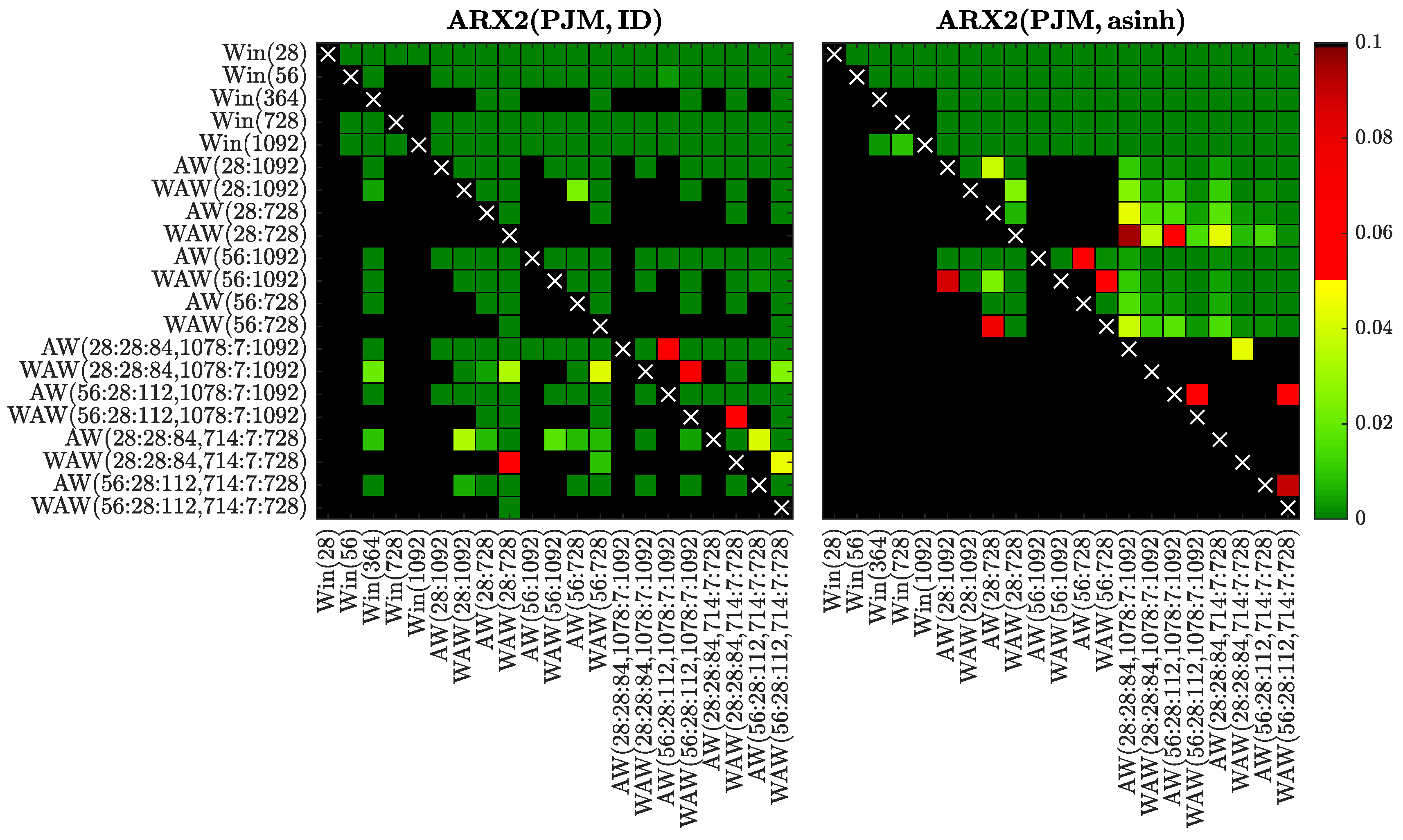
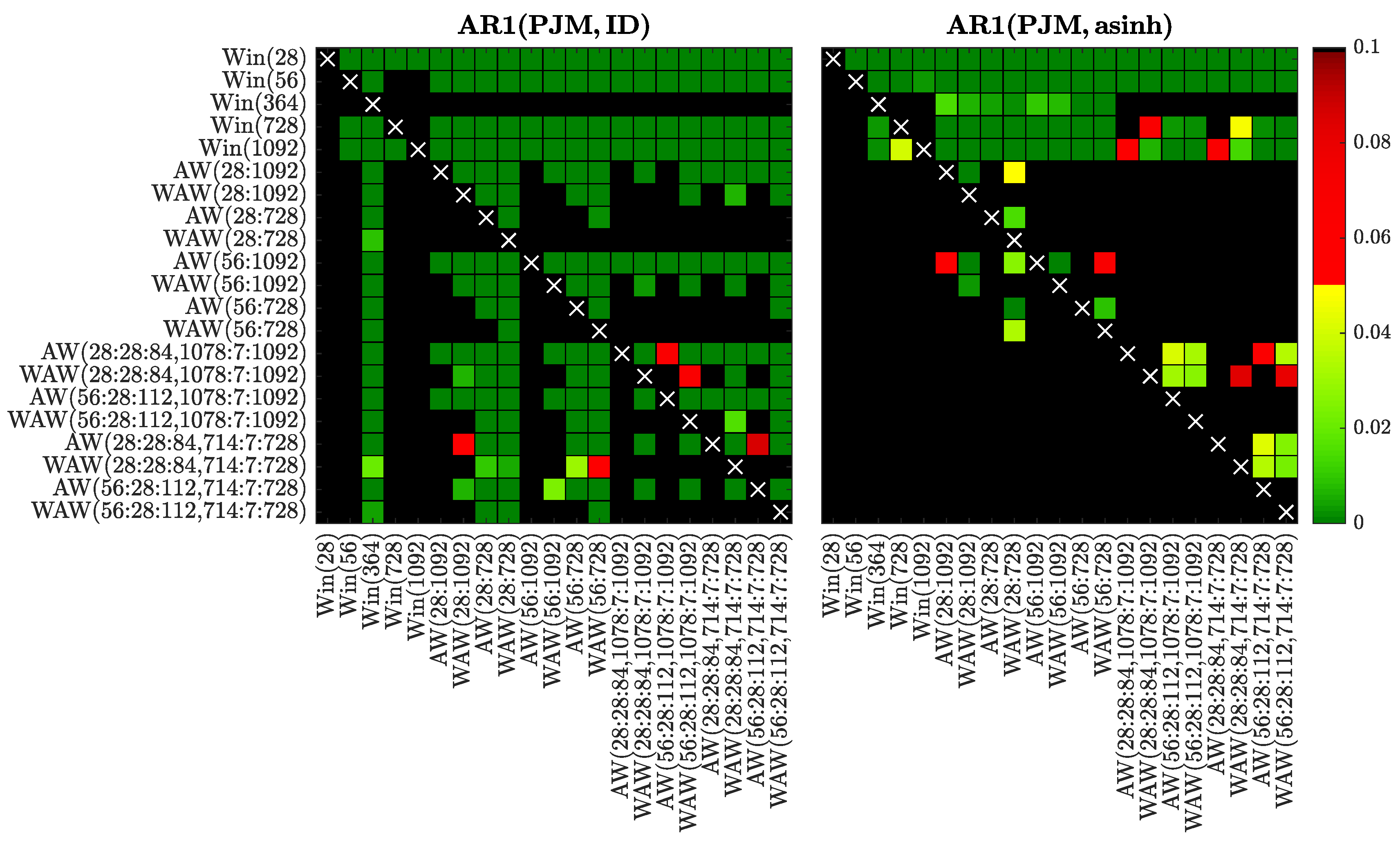
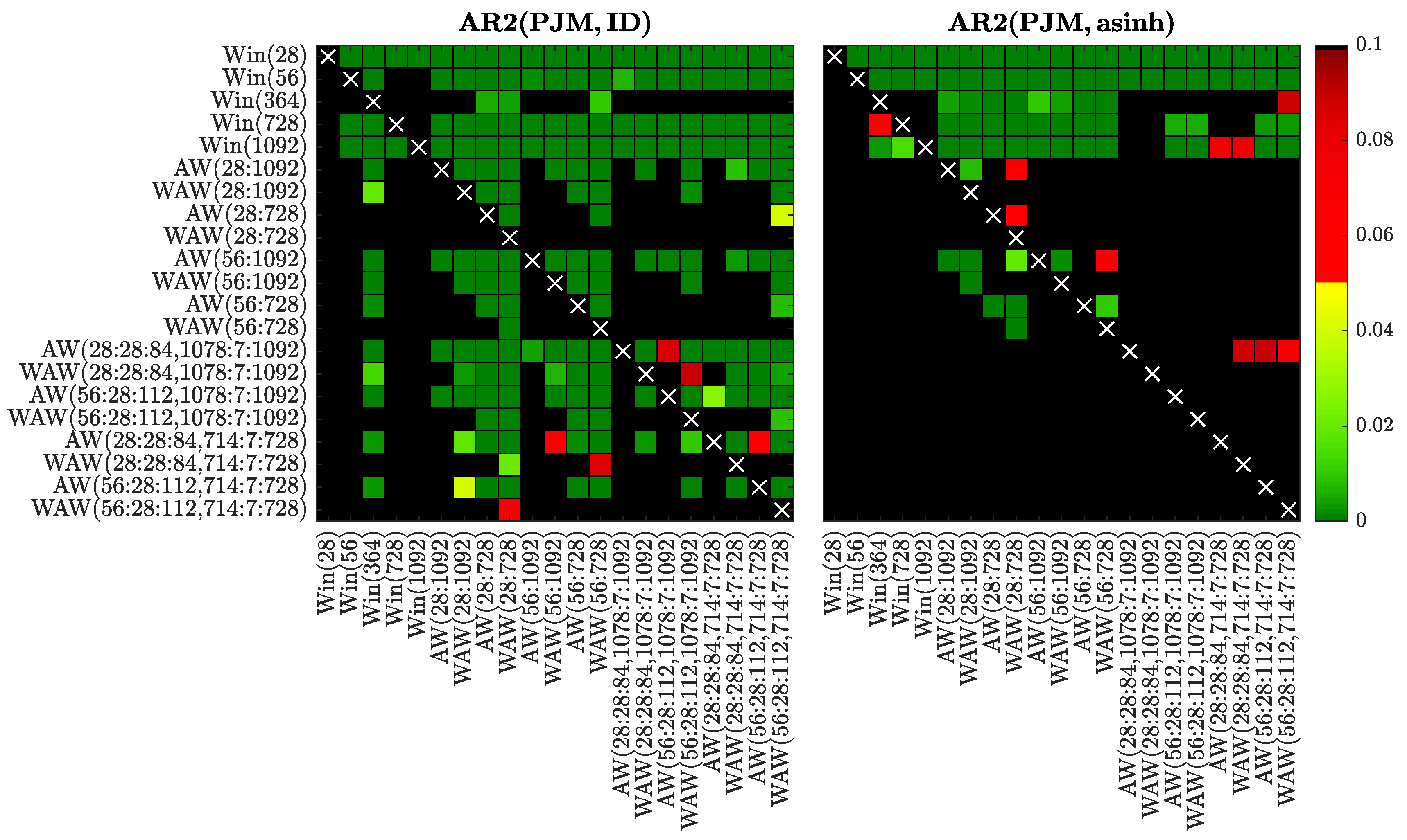
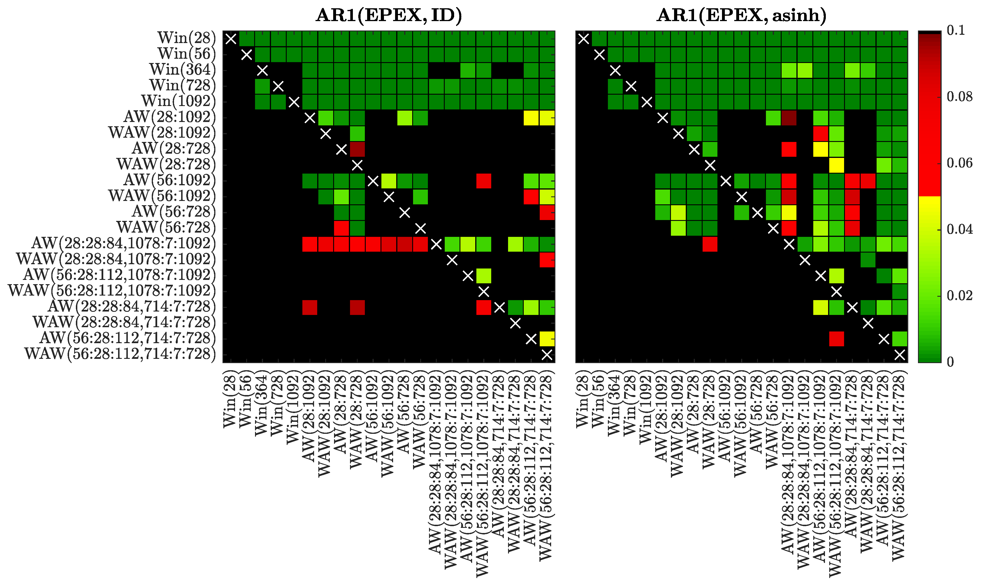
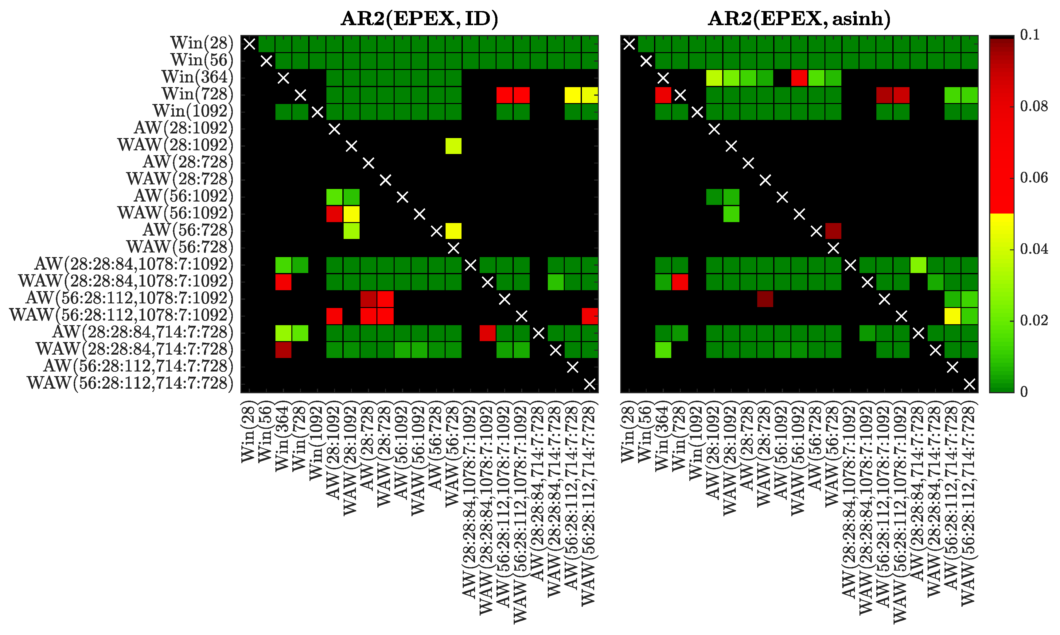
In Figure 8, Figure 9, Figure 10, Figure 11, Figure 12, Figure 13, Figure 14 and Figure 15 we visualize the obtained p-values using ‘chessboards’, analogously as in [18,19,25,26,27] for the Diebold-Mariano test, i.e., we use a heat map to indicate the range of the p-values—the closer they are to zero (→ dark green) the more significant is the difference between the forecasts of a set on the X-axis (better) and the forecasts of a set on the Y-axis (worse). For instance, the first row in the right panels of Figure 8, Figure 9, Figure 10, Figure 11, Figure 12, Figure 13, Figure 14 and Figure 15 is green, indicating that the forecasts of all four expert models for every window set significantly outperform those for Win(28). Actually, in the left panels the first row is also green except for the black squares corresponding to the very poorly performing Win(728) and Win(1092) predictions for the ARX1 model fitted to raw PJM prices, see Figure 10. On the other hand, the columns which correspond to WAW(28:28:84, 1078:7:1092) averaging are green in both panels of Figure 8, meaning that this window set leads to significantly better forecasts than all other for the ARX1 model fitted to ID- or asinh-transformed Nord Pool prices. Note, that due to the explosive nature of models calibrated to asinh-transformed PJM data over very short windows (see Section 3.1), in the right panels of Figure 10, Figure 11, Figure 12 and Figure 13 all window sets were left-truncated at 40 days, i.e., all windows of less than 40 days were discarded from the average for models AW(28:1092) through WAW(28:728), while window $T=28$ was replaced by $T=40$ for the remaining ones.

Overall, the CPA test results confirm and emphasize the observations made in Section 3.1. In particular, the majority of AW and WAW averaged forecasts significantly outperform those of the five selected calibration window lengths, see the mostly green rows corresponding to Win(T)’s for $T=28,56,365,728,1092$. Moreover, in cases such as ARX2(PJM, ID) and ARX2(NP, ID), where some of the Win(T) forecasts are performing well, the T varies. An ex-ante choice of the correct calibration window (respectively 364 and 1092 days in these two cases) is problematic. On the other hand, the averaged forecasts (especially based on the new WAW scheme) are less prone to this instability. The mixed short- and long-term window sets are strong performers in these two cases, and in general across all datasets and models (note the mostly green columns corresponding to these $\mathcal{T}$’s).

Comparing the averaging schemes, it is worth noting that in no case does AW significantly outperform the corresponding WAW scheme. On the other hand, the opposite can be observed for several cases—across all datasets, both transformations and different numbers of averaged forecasts. This result reinforces our recommendation of using the WAW scheme for combining multiple forecasts for EPF, regardless of the number of predictions combined.

Finally, the recommended above WAW(56:28:112, 714:7:728) averaging scheme performs strongly (see the largely green rightmost columns) and—in most cases—is not significantly outperformed by any other model (see the mostly black bottom rows). This is especially worth emphasizing, because the best model is different for almost each of the test cases, see Table 1, Table 2, Table 3 and Table 4 and Figure 4, Figure 5, Figure 6 and Figure 7.

4. Conclusions

In this paper, we report on a comprehensive empirical study on the selection of calibration windows for day-ahead EPF. Our starting point was the paper of Hubicka et al. [30], who proposed a novel concept in energy forecasting that combined day-ahead predictions across different calibration windows. We have extended their analysis to much longer datasets, predictive models with more explanatory variables, VST-transformed price and consumption/load series and—most importantly—introduced a new, well-performing WAW weighting scheme for averaging forecasts.

Firstly, we have confirmed the observations of Ziel and Weron [27], that AR(X)2 is a very competitive expert model, and of Uniejewski et al. [26], that models calibrated to asinh-transformed prices (and consumption/load forecasts) outperform by a large margin structures fitted to raw prices. Since the area hyperbolic sine transformation is straightforward to implement and its computational cost is negligible, we recommend it for EPF.

Moreover, we have shown that the majority of AW and WAW averaged forecasts significantly outperform those obtained from fitting a model to one ex-ante selected window length. Interestingly, in no case did AW significantly outperform the corresponding WAW scheme. On the other hand, the opposite can be observed for several cases—across all datasets, both transformations and different numbers of averaged forecasts.

As noted by Hubicka et al. [30], the mixed short- and long-term window sets are strong performers—in our case, this is true across all datasets and models. However, we suggest to use slightly longer windows at the shorter end, because MAEs may explode for the latter, especially if models with more variables are considered. On the other hand, including 3- instead of 2-year windows does not bring significant benefits. Overall, we recommend the WAW(56:28:112, 714:7:728) averaging scheme. It performs very well and—in most cases—is not significantly outperformed by any other forecast.

References

- Weron, R. Electricity price forecasting: A review of the state-of-the-art with a look into the future. Int. J. Forecast. 2014, 30, 1030–1081. [Google Scholar] [CrossRef]
- Zhao, J.; Dong, Z.; Xu, Z.; Wong, K. A statistical approach for interval forecasting of the electricity price. IEEE Trans. Power Syst. 2008, 23, 267–276. [Google Scholar] [CrossRef]
- Dudek, G. Multilayer perceptron for GEFCom2014 probabilistic electricity price forecasting. Int. J. Forecast. 2016, 32, 1057–1060. [Google Scholar] [CrossRef]
- Zareipour, H.; Canizares, C.A.; Bhattacharya, K.; Thomson, J. Application of public-domain market information to forecast Ontario’s wholesale electricity prices. IEEE Trans. Power Syst. 2006, 21, 1707–1717. [Google Scholar] [CrossRef]
- Conejo, A.J.; Plazas, M.A.; Espinola, R.; Molina, A.B. Day-ahead electricity price forecasting using the wavelet transform and ARIMA models. IEEE Trans. Power Syst. 2005, 20, 1035–1042. [Google Scholar] [CrossRef]
- Amjady, N. Day-ahead price forecasting of electricity markets by a new fuzzy neural network. IEEE Trans. Power Syst. 2006, 21, 887–896. [Google Scholar] [CrossRef]
- Amjady, N.; Keynia, F. Day-ahead price forecasting of electricity markets by mutual information technique and cascaded neuro-evolutionary algorithm. IEEE Trans. Power Syst. 2009, 24, 306–318. [Google Scholar] [CrossRef]
- Voronin, S.; Partanen, J. Price forecasting in the day-ahead energy market by an iterative method with separate normal price and price spike frameworks. Energies 2013, 6, 5897–5920. [Google Scholar] [CrossRef]
- Misiorek, A.; Trück, S.; Weron, R. Point and interval forecasting of spot electricity prices: Linear vs. non-linear time series models. Stud. Nonlinear Dyn. Econom. 2006, 10. [Google Scholar] [CrossRef] [Green Version]
- Weron, R.; Misiorek, A. Forecasting spot electricity prices: A comparison of parametric and semiparametric time series models. Int. J. Forecast. 2008, 24, 744–763. [Google Scholar] [CrossRef] [Green Version]
- Serinaldi, F. Distributional modeling and short-term forecasting of electricity prices by Generalized Additive Models for Location, Scale and Shape. Energy Econ. 2011, 33, 1216–1226. [Google Scholar] [CrossRef]
- Bordignon, S.; Bunn, D.W.; Lisi, F.; Nan, F. Combining day-ahead forecasts for British electricity prices. Energy Econ. 2013, 35, 88–103. [Google Scholar] [CrossRef] [Green Version]
- Nowotarski, J.; Raviv, E.; Trück, S.; Weron, R. An empirical comparison of alternate schemes for combining electricity spot price forecasts. Energy Econ. 2014, 46, 395–412. [Google Scholar] [CrossRef]
- Keles, D.; Scelle, J.; Paraschiv, F.; Fichtner, W. Extended forecast methods for day-ahead electricity spot prices applying artificial neural networks. Appl. Energy 2016, 162, 218–230. [Google Scholar] [CrossRef]
- Maciejowska, K.; Nowotarski, J.; Weron, R. Probabilistic forecasting of electricity spot prices using Factor Quantile Regression Averaging. Int. J. Forecast. 2016, 32, 957–965. [Google Scholar] [CrossRef]
- Nowotarski, J.; Weron, R. On the importance of the long-term seasonal component in day-ahead electricity price forecasting. Energy Econ. 2016, 57, 228–235. [Google Scholar] [CrossRef]
- Uniejewski, B.; Nowotarski, J.; Weron, R. Automated Variable Selection and Shrinkage for Day-Ahead Electricity Price Forecasting. Energies 2016, 9, 621. [Google Scholar] [CrossRef]
- Marcjasz, G.; Uniejewski, B.; Weron, R. On the importance of the long-term seasonal component in day-ahead electricity price forecasting with NARX neural networks. Int. J. Forecast. 2018. [Google Scholar] [CrossRef]
- Uniejewski, B.; Marcjasz, G.; Weron, R. On the importance of the long-term seasonal component in day-ahead electricity price forecasting. Part II—Probabilistic forecasting. Energy Econ. 2018. [Google Scholar] [CrossRef]
- Garcia-Martos, C.; Rodriguez, J.; Sanchez, M. Forecasting electricity prices by extracting dynamic common factors: Application to the Iberian Market. IET Gener. Transm. Distrib. 2012, 6, 11–20. [Google Scholar] [CrossRef]
- Alonso, A.M.; Bastos, G.; Garcia-Martos, C. Electricity price forecasting by averaging dynamic factor models. Energies 2016, 9, 600. [Google Scholar] [CrossRef]
- Ziel, F. Forecasting Electricity Spot Prices Using LASSO: On Capturing the Autoregressive Intraday Structure. IEEE Trans. Power Syst. 2016, 31, 4977–4987. [Google Scholar] [CrossRef]
- Ziel, F.; Steinert, R. Electricity price forecasting using sale and purchase curves: The X-Model. Energy Econ. 2016, 59, 435–454. [Google Scholar] [CrossRef] [Green Version]
- Neupane, B.; LeeWoon, W.; Aung, Z. Ensemble prediction model with expert selection for electricity price forecasting. Energies 2017, 10, 77. [Google Scholar] [CrossRef]
- Uniejewski, B.; Weron, R. Efficient forecasting of electricity spot prices with expert and LASSO models. Energies 2018, 11, 2039. [Google Scholar] [CrossRef]
- Uniejewski, B.; Weron, R.; Ziel, F. Variance Stabilizing Transformations for Electricity Spot Price Forecasting. IEEE Trans. Power Syst. 2018, 33, 2219–2229. [Google Scholar] [CrossRef]
- Ziel, F.; Weron, R. Day-ahead electricity price forecasting with high-dimensional structures: Univariate vs. multivariate modeling frameworks. Energy Econ. 2018, 70, 396–420. [Google Scholar] [CrossRef] [Green Version]
- Maciejowska, K.; Weron, R. Forecasting of daily electricity prices with factor models: Utilizing intra-day and inter-zone relationships. Comput. Stat. 2015, 30, 805–819. [Google Scholar] [CrossRef]
- Fezzi, C.; Mosetti, L. Size Matters: Estimation Sample Length and Performance In Electricity Price Forecasting. Unpublished work. 2018. [Google Scholar]
- Hubicka, K.; Marcjasz, G.; Weron, R. A note on averaging day-ahead electricity price forecasts across calibration windows. IEEE Trans. Sustain. Energy 2018. [Google Scholar] [CrossRef]
- Hong, T.; Pinson, P.; Fan, S.; Zareipour, H.; Troccoli, A.; Hyndman, R.J. Probabilistic energy forecasting: Global Energy Forecasting Competition 2014 and beyond. Int. J. Forecast. 2016, 32, 896–913. [Google Scholar] [CrossRef] [Green Version]
- Giacomini, R.; White, H. Tests of conditional predictive ability. Econometrica 2006, 74, 1545–1578. [Google Scholar] [CrossRef]
- Janczura, J.; Trück, S.; Weron, R.; Wolff, R. Identifying spikes and seasonal components in electricity spot price data: A guide to robust modeling. Energy Econ. 2013, 38, 96–110. [Google Scholar] [CrossRef] [Green Version]
- Schneider, S. Power spot price models with negative prices. J. Energy Mark. 2011, 4, 77–102. [Google Scholar] [CrossRef] [Green Version]
- Gaillard, P.; Goude, Y.; Nedellec, R. Additive models and robust aggregation for GEFCom2014 probabilistic electric load and electricity price forecasting. Int. J. Forecast. 2016, 32, 1038–1050. [Google Scholar] [CrossRef]
- Kristiansen, T. Forecasting Nord Pool day-ahead prices with an autoregressive model. Energy Policy 2012, 49, 328–332. [Google Scholar] [CrossRef]
- Weron, R. Modeling and Forecasting Electricity Loads and Prices: A Statistical Approach; John Wiley & Sons: Chichester, UK, 2006. [Google Scholar]
- Maciejowska, K.; Nowotarski, J. A hybrid model for GEFCom2014 probabilistic electricity price forecasting. Int. J. Forecast. 2016, 32, 1051–1056. [Google Scholar] [CrossRef]
- Gianfreda, A.; Parisio, L.; Pelagatti, M. A review of balancing costs in Italy before and after RES introduction. Renew. Sustain. Energy Rev. 2018, 91, 549–563. [Google Scholar] [CrossRef]
- Pesaran, M.; Timmermann, A. Selection of estimation window in the presence of breaks. J. Econ. 2007, 137, 134–161. [Google Scholar] [CrossRef] [Green Version]
- Pesaran, M.; Pick, A. Forecast combination across estimation windows. J. Bus. Econ. Stat. 2011, 29, 307–318. [Google Scholar] [CrossRef] [Green Version]
- Nowotarski, J.; Liu, B.; Weron, R.; Hong, T. Improving short term load forecast accuracy via combining sister forecasts. Energy 2016, 98, 40–49. [Google Scholar] [CrossRef]
- Liu, B.; Nowotarski, J.; Hong, T.; Weron, R. Probabilistic load forecasting via Quantile Regression Averaging on sister forecasts. IEEE Trans. Smart Grid 2017, 8, 730–737. [Google Scholar] [CrossRef]
- Stock, J.H.; Watson, M.W. Combination forecasts of output growth in a seven-country data set. J. Forecast. 2004, 23, 405–430. [Google Scholar] [CrossRef]
- Diebold, F.X.; Mariano, R.S. Comparing predictive accuracy. J. Bus. Econ. Stat. 1995, 13, 253–263. [Google Scholar]
- Giacomini, R.; Rossi, B. Forecasting in Macroeconomics. In Handbook of Research Methods and Applications on Empirical Macroeconomics; Hashimzade, N., Thornton, M., Eds.; Edward Elgar: Cheltenham, UK, 2013; pp. 381–407. [Google Scholar]
Figure 1.
Nord Pool (NP) hourly system prices (top) and hourly consumption prognosis (bottom) from 1 January 2013 to 31 July 2018. The vertical dashed lines mark the end of the initial 1092-day calibration window (i.e., 1 January 2013–28 December 2015). Weights for the WAW approach (see Section 2.5) are selected based on price predictions for the following day (i.e., 29 December 2015 for the initial calibration windows) and the remaining observations constitute the 945-day out-of-sample test period.
Figure 2.
PJM hourly prices (top) and hourly consumption prognosis (bottom) in the Commonwealth Edison (COMED) zone from 10 April 2012 to 2 April 2018. The vertical dashed lines mark the end of the initial 1092-day calibration window (i.e., 10 April 2012–6 April 2015). Weights for the WAW approach are selected based on price predictions for the following day (i.e., 7 April 2015 for the initial calibration windows) and the remaining observations constitute the 1091-day out-of-sample test period.
Figure 3.
EPEX hourly system prices for Germany and Austria from 6 August 2010 to 28 July 2016. The vertical dashed lines mark the end of the initial 1092-day calibration window (i.e., 6 August 2010–1 August 2013). Weights for the WAW approach are selected based on price predictions for the following day (i.e., 2 August 2013 for the initial calibration windows) and the remaining observations constitute the 1091-day out-of-sample test period.
Figure 4.
Mean absolute errors (MAE) for the Nord Pool (NP) dataset as a function of the window length (gray circles) and obtained by combining forecasts: solid lines for AW() and dashed lines for WAW() averages across all windows in a given range, solid lines with symbols for AW() and dashed lines with symbols for WAW() averages with cherry-picked windows. MAEs are plotted for ARX1 (top) and ARX2 models (bottom), calibrated to raw (left) and asinh-transformed prices (right). Note the different scales. Out-of-range lines or symbols are not visible.
Figure 5.
Mean absolute errors (MAE) for the PJM dataset as a function of the window length (gray circles) and obtained by combining forecasts (the color/line/symbol scheme and the location of panels is the same as in Figure 4). Note the different scales. Out-of-range lines or symbols are not visible.
Figure 6.
Mean absolute errors (MAE) for the PJM dataset as a function of the window length (gray circles) and obtained by combining forecasts (the color/line/symbol scheme is the same as in Figure 4). MAEs are plotted for AR1 (top) and AR2 models (bottom), calibrated to raw (left) and asinh-transformed prices (right). Note the different scales. Out-of-range lines or symbols are not visible.
Figure 7.
Mean absolute errors (MAE) for the EPEX dataset as a function of the window length (gray circles) and obtained by combining forecasts (the color/line/symbol scheme and the location of panels is the same as in Figure 6). Note the different scales. Out-of-range lines or symbols are not visible.
Figure 8.
Results of the conditional predictive ability (CPA) test [32] for selected window sets and the ARX1 model fitted to raw (left) or asinh-transformed (right) Nord Pool data. We use a heat map to indicate the range of the p-values – the closer they are to zero (→ dark green) the more significant is the difference between the forecasts of a set on the X-axis (better) and the forecasts of a set on the Y-axis (worse).
Figure 9.
Results of the CPA test for selected window sets and the ARX2 model fitted to raw (left) or asinh-transformed (right) Nord Pool data. We use a heat map to indicate the range of the p-values—the closer they are to zero (→ dark green) the more significant is the difference between the forecasts of a set on the X-axis (better) and the forecasts of a set on the Y-axis (worse).
Figure 10.
Results of the CPA test for selected window sets and the ARX1 model fitted to raw (left) or asinh-transformed (right) PJM data. We use a heat map to indicate the range of the p-values—the closer they are to zero (→ dark green) the more significant is the difference between the forecasts of a set on the X-axis (better) and the forecasts of a set on the Y-axis (worse).
Figure 11.
Results of the CPA test for selected window sets and the ARX2 model fitted to raw (left) or asinh-transformed (right) PJM data. We use a heat map to indicate the range of the p-values—the closer they are to zero (→ dark green) the more significant is the difference between the forecasts of a set on the X-axis (better) and the forecasts of a set on the Y-axis (worse).
Figure 12.
Results of the CPA test for selected window sets and the AR1 model fitted to raw (left) or asinh-transformed (right) PJM prices. We use a heat map to indicate the range of the p-valuesthe closer they are to zero (→ dark green) the more significant is the difference between the forecasts of a set on the X-axis (better) and the forecasts of a set on the Y-axis (worse).
Figure 13.
Results of the CPA test for selected window sets and the AR2 model fitted to raw (left) or asinh-transformed (right) PJM prices. We use a heat map to indicate the range of the p-values—the closer they are to zero (→ dark green) the more significant is the difference between the forecasts of a set on the X-axis (better) and the forecasts of a set on the Y-axis (worse).
Figure 14.
Results of the CPA test for selected window sets and the AR1 model fitted to raw (left) or asinh-transformed (right) EPEX prices. We use a heat map to indicate the range of the p-values—the closer they are to zero (→ dark green) the more significant is the difference between the forecasts of a set on the X-axis (better) and the forecasts of a set on the Y-axis (worse).
Figure 15.
Results of the CPA test for selected window sets and the AR2 model fitted to raw (left) or asinh-transformed (right) EPEX prices. We use a heat map to indicate the range of the p-values—the closer they are to zero (→ dark green) the more significant is the difference between the forecasts of a set on the X-axis (better) and the forecasts of a set on the Y-axis (worse).