A Trading-Based Evaluation of Density Forecasts in a Real-Time Electricity Market

Abstract

This paper applies a multi-factor, stochastic latent moment model to predicting the imbalance volumes in the Austrian zone of the German/Austrian electricity market. This provides a density forecast whose shape is determined by the flexible skew-t distribution, the first three moments of which are estimated as linear functions of lagged imbalance and forecast errors for load, wind and solar production. The evaluation of this density predictor is compared to an expected value obtained from OLS regression model, using the same regressors, through an out-of-sample backtest of a flexible generator seeking to optimize its imbalance positions on the intraday market. This research contributes to forecasting methodology and imbalance prediction, and most significantly it provides a case study in the evaluation of density forecasts through decision-making performance. The main finding is that the use of the density forecasts substantially increased trading profitability and reduced risk compared to the more conventional use of mean value regressions.

1. Introduction

Motivated by the requirements for accurate risk management, forecasting the density functions for electricity prices and loads is attracting an increased amount of research into new methodologies. Substantial overviews on the related literature are given in references [1,2]. For example, Jónsson et al. [3] applied exponential smoothing approaches for prediction in real-time electricity markets, Bello et al. [4] analyzed Parametric Density Recalibration of a Fundamental Market Model to Forecast Electricity Prices, Chan and Grant [5] compared energy price dynamics with GARCH and stochastic volatility models, Jiang et al. [6] forecasted day-ahead electricity prices based on a hybrid model applying particle swarm optimization and core mapping with fuzzy logic and model selection, Uniejewski et al. [7] show how variance stabilizing transformations can improve electricity spot price forecasting and Hagfors et al. [8] used quantile regressions to forecast UK electricity prices. Most recently, techniques from the field of artificial intelligence have been evaluated with success. Thus, Lago et al. [9] used various deep learning approaches and compared them to traditional algorithms/forecasting methods, Singh & Yassine and Gajowniczek & Ząbkowski [10,11] applied big data mining and machine learning algorithms to load forecasting and Wang et al. [12] applied a deep learning algorithm based on the assembly approach to forecast probabilistic wind power production using quantile regression. In references [13,14], the authors developed hybrid models combining ARIMA, kernel-based extreme learning machine and neural networks to forecast day and week ahead electricity prices.

However, as Weron [2] observes, most of this work has taken the form of point or interval forecasting, e.g., with quantile regressions, as in reference [8,12] or [15], rather than through fully parametric density representations, and almost all of it has been in the context of short-term, day-ahead modeling. Of the parametric representations for hourly prices, Panagiotelis and Smith [16] applied a skew-t distribution, Serinaldi [17] used the JSU, while Gianfreda and Bunn [18] found that the skew-t was preferable to the JSU. However, an enduring question with density forecasting has been how to evaluate its benefits. Generally, the in-sample fits and the out-of-sample forecasts are assessed through conversion of the densities to intervals and then testing the intervals for calibration, as in [18]. Some researchers have implemented the average log predictive score or the average continuous ranked probability score (CRPS), as in reference [19]. However, more commonly used in practice is the value-at-risk backtesting procedure, whereby for example the 5%, 95% quantile predictions are expected to cover 5% and 95% of the outcomes ex post (see the coverage tests and references [20,21]).

Nevertheless, while such tests of calibration are useful for comparing the specification of different densities, the overall question of the usefulness of the full density representation, compared to expected values, remains under-researched in the context of short-term electricity decision-making. This paper therefore seeks to provide new empirical evidence for the value of density forecasting, through assessing intraday trading performance with and without full density specifications. In doing so, we approximate the full density with 21 quantiles, aware that this is a limitation with respect to the whole 99 percentiles; for a deeper discussion on the topic see references [1,22]. The main objective of this research is therefore to evaluate quantile forecasts by means of trading payoffs.

Surprisingly, while there is an extensive research literature on the relative merits of different measures of forecast accuracy, evaluating electricity price forecasts in general, from the perspective of decision-making effectiveness has rarely been undertaken. Slightly more has appeared with respect to loads and production, than for predicting prices. Thus, Kraas et al. [23] show the economic value of short-term electricity trading using a forecasting system for solar production compared to a naïve heuristic, and Barthelmie, Murray and Pryor [24] demonstrate similar benefits to the operators of wind farms who use more accurate wind speed predictors. Zareipour et al. [25] studied the economic impact of electricity market price forecast inaccuracies to short-term operation scheduling for two industrial loads using point forecasts. With respect to the more focused question of using a mean-value predictor versus a density function, the intuition has always been that it is context-dependent and, in particular, it relates to whether the recourse costs of the forecast errors are symmetric.

This paper therefore provides two contributions:

• Firstly, the value of forecasting with densities, compared to mean-values, is shown, through back-testing real-time trading strategies on the Austrian balancing zone of the German/Austrian electricity market,
• Secondly, a new density modeling technique, previously only applied to prices, is extended successfully to forecasting the imbalance volumes at 15 min resolution, and outperforms a more conventional benchmark.

The paper is organized as follows: the next section describes the application context, followed by the predictive methodology in Section 3. Section 4 presents the optimal imbalance positions, whereas the results on backtesting the optimal trading strategies are described in Section 5. Finally, Section 6 concludes.

2. The Austrian Balancing Market

The German/Austrian intraday power exchange is operated by EPEX Spot SE and the power market area comprises 5 delivery zones managed by 5 Transmission System Operators (TSOs), one of which is the Austrian Power Grid (APG). Intraday trading occurs continuously 7 days a week and the five delivery zones are traded from one order book. The basic intraday delivery period is 15 min, which can be traded until 30 min before delivery begins. For the Austrian delivery zone, internal schedule changes (within the zone) are allowed up to 15 min before delivery (but international flows require 45 min notice). APG publishes the preliminary estimate of system imbalance every 15 min, with a lag of 10 min. A detailed description of the information flow is presented in [26]. APG is part of the synchronized European grid and follows the standard process of acquiring control power to ensure the frequency stability and operational security. Primary and Secondary control power is deployed automatically within 30 s and 5 min, respectively, while Tertiary is activated by the TSO on a 15 min basis to replace the Secondary reserves.

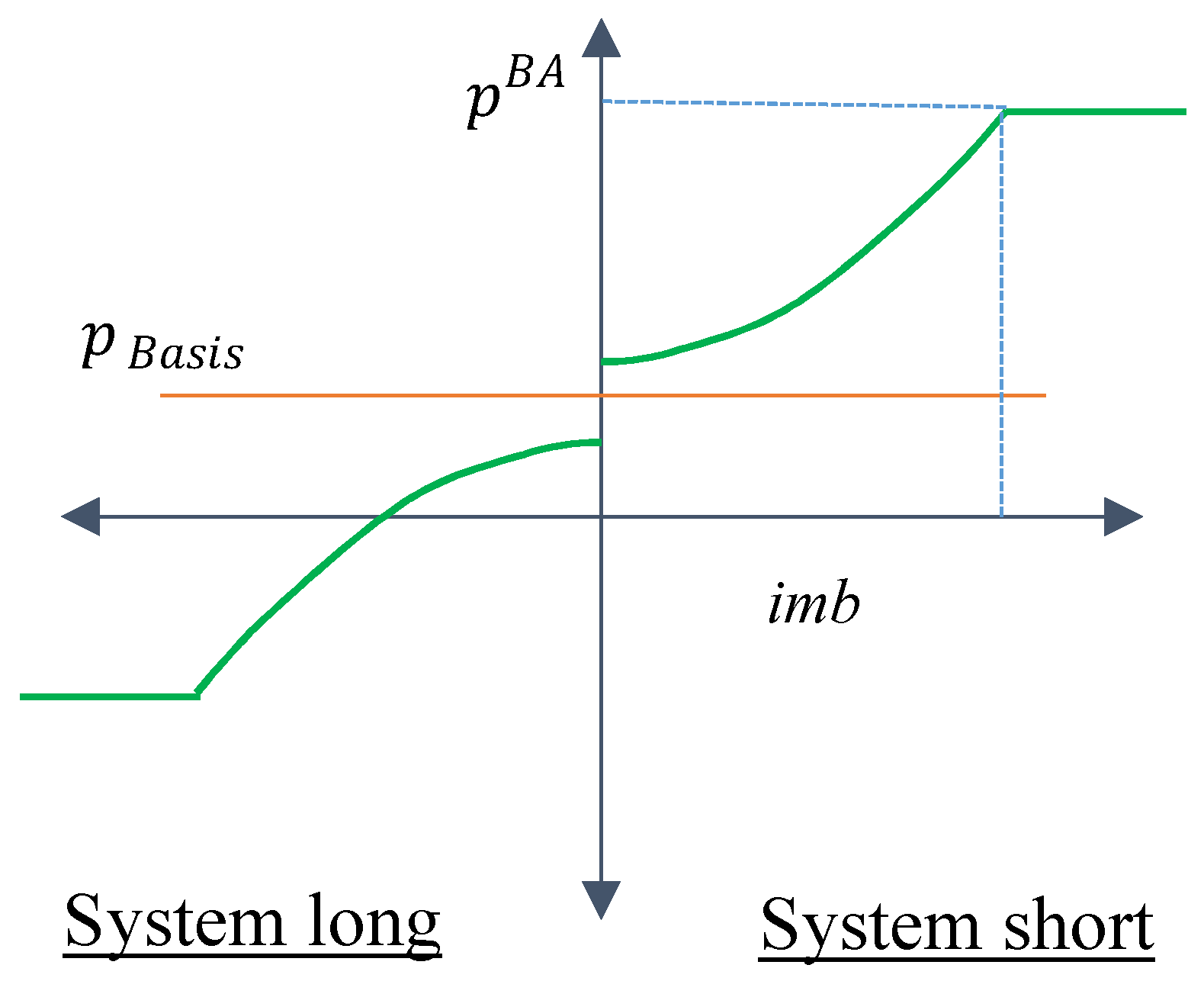
Austria has a single price, imbalance settlement design. Unlike its coupled neighbor, Germany, where despite a single price balancing market, the parties responsible for balancing are contractually obliged to keep schedules in balance, the Austrian market rules do not prohibit deliberate short or long positions in the real-time balancing market. Similar to in Britain, and for physical players in Belgium, participants can take out-of-balance positions if they expect to make a profit, and in so doing benefit the system as well. The Imbalance (imb) of the system for a delivery period is the deficit or surplus of load compared to the aggregate nominated values by the market participants. The Austrian Balancing Group Coordinator APCS is responsible for setting up and clearing the balancing system in Austria. The balancing price p^BA for these imbalances is determined from a “basis price” and a “transfer function”. The basis price p^Basis is

$$p^{Basis}\{\begin{array}{l}min\left(p^{tert},p^{ID},p^{DA}\right)\mathrm{for}imb<0\mathrm{and}\mathrm{activated}\mathrm{tertiary}\\ min\left(p^{ID},p^{DA}\right)\mathrm{for}imb<0\mathrm{and}\mathrm{no}\mathrm{tertiary}\\ max\left(p^{tert},p^{ID},p^{DA}\right)\mathrm{for}imb>0\mathrm{and}\mathrm{activated}\mathrm{tertiary}\\ max\left(p^{ID},p^{DA}\right)\mathrm{for}imb>0\mathrm{and}\mathrm{no}\mathrm{tertiary}\end{array}$$

(1)

where $p^{ID}$ is the hourly average intraday price for that 15 min period as traded previously on the wholesale power exchange (EPEX Spot), $p^{DA}$ is the previous relevant hourly day-ahead auction price (administered by EXAA) and $p^{tert}$ is the volume-weighted average price for any activated tertiary control power in that 15 min delivery period. The “transfer function” is defined as

$$T=\min (U_{min}+\frac{U_{max}-U_{min}}{im{b}_{max}^2}\times {imb}^2;U_{max})$$

(2)

where U_max = 40 €/MWh and U_min = 3 €/MWh, being the fixed maximum and minimum parameter values of the transfer function $T$for the monthly data in our analysis. These values are set by the Energy Regulatory Authority (ERA) and are adapted from time to time. The ex post balancing price is then:

$$p^{BA}=p^{Basis} \pm T$$

(3)

Figure 1 shows graphically the principle of the price mechanism. Depending on the state of the imbalance, the balancing price function follows a quadratic term within the range $\pm im{b}_{max}$ and is constant for the outer ranges $|imb| \ge im{b}_{max}=70 \mathrm{MWh}$, with this threshold again being set by the ERA. The transfer function is positive if the imbalance of the system is positive, and vice versa for negative.

In addition, and for the aim of the paper, the wind and solar forecast errors (fwind and fsolar, respectively) together with the load forecast error (fload) are considered, and calculated as the difference between the day ahead forecasts and the latest values measured. Wind and solar day-ahead forecasts and outcome data was retrieved from Zentralanstalt für Meteorologie und Geodynamik ZAMG. Imbalance and load data was downloaded from the Austrian TSO APG. Forecast data is only available in hourly resolution while realization values are in 10 min resolution, and so the values were linearly interpolated into 15 min intervals covering the full year 2015, for a total of 35,040 observations.

The trading opportunity offered in Austria is for market participants to anticipate whether the balancing market will be long or short, and then optimize a physical position of going out of balance in the opposite direction. Thus, if a generator spills power (produces more than nominated) when the system is short, it will receive the Imbalance price for the volume spilled, which will be higher than if it had previously sold that volume in the power exchange. Whether the regulatory codes permit this deliberate imbalancing varies by jurisdiction: in Austria, Belgium, the Netherlands and the UK, it is permitted, but not so in Germany and France. Thus, in the Austrian case, participants may find it opportunistic, and to take advantage, they will need an adequate predictive method for the imbalance volumes.

Assuming a player is seeking to maximize the expected value according to a spillage or shortage strategy, it is crucial to have relevant predictive information about the probability. In this way, the optimal player’s decision will depend on the imbalance estimates and on the anticipated price responses. Thus, the 15 min imbalance data were firstly analyzed over 2015 to elucidate statistical properties and distributional features, and then a range of possible predictive factors for the expected imbalance variable at time t, ${\widehat{imb}}_t,$ were considered.

3. Data Analysis and Predictive Methodology

Descriptive statistics for observed imbalances are reported in

Table 1. Descriptive statistics for imbalance data over 2015 and calendar seasons.

	Whole Year	Winter	Spring	Summer	Autumn
		(Dec.–Feb.)	(Mar.–May)	(Jun.–Aug.)	(Sept.–Nov.)
Average	0.131	.629	−4.877	0.316	5.753
Maximum	151.146	131.480	138.899	151.146	140.798
Minimum	−320.021	−205.058	−197.641	−320.021	−230.439
Standard Deviation	33.525	31.638	36.503	33.325	31.482
Skewness	−0.834	−0.637	−0.566	−1.631	−0.387
Kurtosis	6.904	5.151	4.644	12.186	5.757
JB statistics	26311	2250	1466	34967	2986

, where minimum and maximum values are reported together with sample mean, standard deviation, skewness, kurtosis, and the Jarque-Bera JB statistics under the normality assumption. It is possible to observe that the maximum short system position was about 320 MWh, whereas the maximum long system position was about 150 MWh. More importantly, these imbalance series do not follow a normal distribution (given that the null is always rejected). Therefore, the 15 min imbalance data is examined in order to find the best fitting distribution.

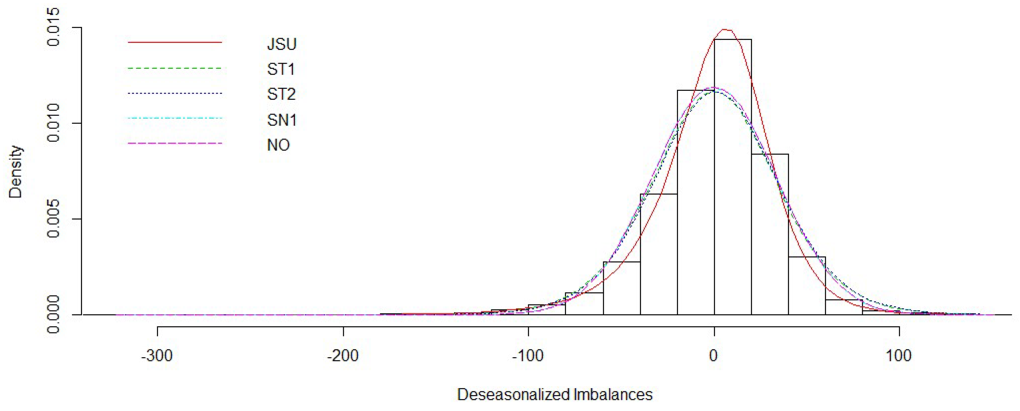
The first class of distribution considered were the 4-parameter distributions: the Johnson’s S_U (in its alternative parametrization as in reference [27], JSU), the sinh-arcsinh (as in reference [28], see SHASHo and SHASHo2), the skew-t (as in references [29,30,31], respectively ST1, ST2 and ST5). The second class is a 3-parameter family represented by the skew-normal distributions, specifically the skew normal ‘type 1’ (SN1), which is a special case of the skew exponential power with τ = 2. Thirdly, selected as a baseline, the 2-parameter normal distribution (NO) as this is often used for simplicity in operational models. Figure 2 presents the density fits for best fitting distributions, after the time series for imbalances have been seasonally adjusted for daily frequency (by using dummy variables for days of the week, from Monday to Saturdays, and holidays).

On the balance of fit, both the Skew-t and the Johnson’s S_U (JSU) distributions seem to be the most appropriate to the series of imbalances. For this purpose, three measures for assessing the goodness-of-fit have been considered, specifically: the Kolmogorov-Smirnov (KS), the Cramér–von Mises (CVM), and the Anderson–Darling (AD). The Anderson–Darling and Cramér–von Mises statistics belong to the class of quadratic statistics, using the squared and the weighted squared differences between the empirical distribution function and the cumulative distribution function of the supposed reference distribution. Hence, both statistics place more weight on observations in the tails of the distribution, with weights being larger for the AD than for the CVM. On the contrary, the Kolmogorov–Smirnov statistic quantifies the absolute maximum distance between the empirical distribution function and the cumulative distribution function of the supposed reference distribution. Therefore, given the observed statistical properties of imbalances series with almost zero asymmetry and moderate kurtosis (especially compared to electricity prices), the latter measure should be preferred. According to results reported in

Table 2. Goodness-of-fit statistics for selected distributions.

	SHASHo	SHASHo2	JSU	ST1	ST2	ST5	SN1	NO
AD	Infinity	4208.7000	0.2900	315.9700	297.4300	6654.8900	244.5600	244.5600
CVM	7474.8600	860.8500	0.0307	51.7100	45.8900	1296.4100	40.5800	40.5800
KS	0.6600	0.2700	0.0020	0.0590	0.0520	0.3570	0.0550	0.0550

, the general superiority of the JSU and the skew student-t distributions (specifically ST2) is observed (note that computational difficulties can emerge, as with infinite values for the SHASHo distribution), consistent with Hagfors et al. [8] for hourly electricity prices.

Furthermore, given that the skew-t had previously also been used for hourly Australian prices in reference [6], while reference [7] used the Johnson’s S_U distribution for Californian and Italian electricity price densities, both distributions have been retained to test their forecasting performances.

However, although the JSU appears to fit slightly better, the backtesting trading results out-of-sample reported later showed better performance for the ST2. Therefore, only the ST2 estimation is described in detail.

Regarding the skew-t variants, comparing their performances, the second skew-t has been selected. The pdf of the skew-t type 2 distribution is denoted by ST2 (µ, σ, υ, τ), conditional on its first four moments. Analytically it can be represented as

$$f_Y\left(y|\mu ,\sigma ,\upsilon ,\tau \right)=\frac{2}{\sigma }{f}_{Z_1}\left(z\right)F_{Z_2}\left(\omega \right)\mathrm{for}-\infty <y<+\infty$$

(4)

where $-\infty <\mu <+\infty$, $\sigma >0$, $-\infty <\upsilon <+\infty$ and $\tau >0$, and where $z=\frac{y-\mu }{\sigma }$, $\omega =\upsilon {\lambda }^{\frac{1}{2}}z$, $\lambda =\frac{\tau +1}{\tau +z^2}$ and $f_{Z_1}$ is the pdf of $Z_1~TF\left(0,1,\tau \right)$, which is a t distribution with $\tau >0$ degrees of freedom treated as a continuous parameter, and $F_{Z_2}$ is the cdf of $Z_2~TF\left(0,1,\tau +1\right)$.

Turning to the predictive factors for the expected imbalance, it is important to recall the actual timing and information flow to simulate predictive decision-making under real operational conditions. The TSO publishes the latest information on imbalance 10 min after the previous delivery period. Based on that information and the latest load, wind and solar forecast errors, the flexible market player can make a decision to up- or down-regulate. Therefore, a minimum information time delay of 30 min is (conservatively) assumed, i.e., a rational expectation lags by two periods t − 2 (including the delivery period itself).

The predictive variables proved to be statistically significant were:

• $im{b}_{t-2}$ is the imbalance variable with a time lag of 2,
• $fwin{d}_{t-2}$ is the wind forecast error, calculated as the difference between the day-ahead forecast and the latest value measured at (t − 2),
• $floa{d}_{t-2}$ is the load forecast error, calculated as the difference between the day-ahead forecast and the latest value measured at (t − 2), and
• $fsola{r}_{t-2}$ is the solar forecast error, calculated as the difference between the day-ahead forecast and the latest value measured at (t − 2).

The 15 min electricity imbalance is formulated as an ST2 density function whose first three moments (and hence its shape) vary according to these exogenous factors.

A similar methodology applied to the German hourly electricity prices has shown that the density shapes are indeed affected by fundamental factors, including wind and solar forecasts. Specifically, [18] showed that forecasted demand, wind and solar PV generation, together with other drivers, were observed to act as “shape-shifters”. More importantly, they provide evidence that modeling all four moments produced marginal and trivial gains in terms of model fitting and out-of-sample forecasting was better without the estimation error of the fourth parameter. Therefore, based on these results, a response variable to the exogenous factors is presented as a skew-t density with the mean, µ, standard deviation, σ, and skewness, υ, modeled as multifactor linear functions as follows (with kurtosis, τ, being kept constant).

Formally, the dynamic multi-factor skew-t model in its autoregressive formulation over the first three moments (AR-MFST-3) has a time-arying latent mean, dispersion and skewness, estimated dynamically as follows:

$${\mu }_t={\alpha }_1+{\gamma }_1{\mu }_{t-1}+{\beta }_{11}im{b}_{t-2}+{\beta }_{12}floa{d}_{t-2}+{\beta }_{13}fwin{d}_{t-2}+{\beta }_{14}fsola{r}_{t-2}$$

(5)

$$\log ({\sigma }_t)={\alpha }_2+{\gamma }_2{\sigma }_{t-1}+{\beta }_{21}im{b}_{t-2}+{\beta }_{22}floa{d}_{t-2}+{\beta }_{23}fwin{d}_{t-2}+{\beta }_{24}fsola{r}_{t-2}$$

(6)

$${\upsilon }_t={\alpha }_3+{\gamma }_3{\upsilon }_{t-1}+{\beta }_{31}im{b}_{t-2}+{\beta }_{32}floa{d}_{t-2}+{\beta }_{33}fwin{d}_{t-2}+{\beta }_{34}fsola{r}_{t-2}$$

(7)

The fourth moment, kurtosis τ, is kept constant for robustness out-of-sample. Adopting a two-stage approach, all moment equations are first estimated on the full sample as specified in Equations (4)–(6) without the autoregressive terms. Then, the lagged filtered series were used to initialize the autoregressive terms, which were later used and updated in the one-step-ahead forecasting process through a rolling procedure with a window size of one week (that is 672 observations as for 4 quarter-hours × 24 hours × 7 days). The filtered values for the constant kurtosis were used to compute the values of the probability density function for both ST2 and JSU. Evidently, the estimated values are constant over the window, but they do change over the rolled windows. These forecasts were subsequently used firstly to compute the ST (and JSU) density function values over a sequence of 200 values for imbalances, constrained between ±500 MW (supported by the observed statistics) with a step of 5 MW. Hence, 34,366 forecasted densities (computed from the original series length of 35,040 observations, excluding the two time lags and subtracting the rolling window size of 672 observations) were approximated, one for each 15 min period included in our sample. The gamlss R package has been used for the estimation and forecasting. For further details and algorithms settings see reference [6]; also [16] and [17].

Secondly, to assess the precision of both predictive distributions (that is, the “sharpness”, as well as the “calibration”), the “pinball loss” was computed, as suggested by reference [32]. Precisely, the following sequence was considered from the 1st to the 99th percentile, with a step of 0.05: 0.01, 0.05, 0.10, 0.15, 0.20, 0.25, 0.30, 0.35, 0.40, 0.45, 0.50, 0.55, 0.60, 0.65, 0.70, 0.75, 0.80, 0.85, 0.90, 0.95, 0.99. Thus, having 21 time series of forecasted quantiles, 34,366* pinball values were computed over the ‘rolling ahead’ forecast horizon (that is, the full sample minus the first 674 observations) and averaged over the forecasting sample. The computation of quantiles from densities simulated according to the forecasted parameters of the JSU distribution led to several unavailable or infinite values: over 34366 forecasts, 330 computational errors were detected for the 1st percentile; 336 for the 5th; 361 for the 10th; 388 for the 15th; 452 for the 20th; 527 for the 25th; 591 for the 30th; 677 for the 35th; 747 for the 40th; 849 for the 45th; and finally, 1024 for all remaining percentiles. Hence, the averages were computed accordingly. Whereas similar problems were not encountered with the ST2 forecasted parameters. Their mean values for each quantile are reported for both distributions in

Table 3. Pinball scores for tested distributions.

	Percentiles
	1	5	10	15	20	25	30	35	40	45	50
JSU	1.1105	3.1324	4.9126	6.2800	7.3589	8.2189	8.8851	9.3779	9.7175	9.9177	9.9832
ST2	0.9817	2.9732	4.7045	6.0299	7.0642	7.8750	8.4990	8.9629	9.2725	9.4502	9.4893
	Percentiles
	55	60	65	70	75	80	85	90	95	99	Average
JSU	9.9163	9.6987	9.3224	8.7776	8.0552	7.1444	6.0174	4.6109	2.8202	0.8550	6.9577
ST2	9.3875	9.1468	8.7631	8.2270	7.5387	6.6794	5.6191	4.3038	2.6368	0.7693	6.5892

, and also reported are their overall averages, computed across all percentiles. In addition, following [32], the pinball scores have been used to denote the estimated forecasting errors ${\widehat{\epsilon }}_{dist,t,q_i}$ for both distributions (dist = ST2; JSU), across all points in time t and quantiles q_i = 1, 5, 10, …, 99 for i = 1, …, 21. Then, the values of these series have been used in the Diebold and Mariano (DM) test with the null hypothesis of equal performance versus the alternative one that JSU is less accurate than ST2; adjusting for missing values and with the differential loss function defined as ${\mathsf{\Delta }}_{ST2, JSU,t,q_i}={\widehat{\epsilon }}_{ST2,t,q_i}- {\widehat{\epsilon }}_{JSU,t,q_i}$; in practice, nominal values instead of absolute ones are used for the estimated forecasting errors, given that the pinball scores are always positive. Results of the DM test show that the null of equal performance is always rejected (in favor of the alternative of JSU being less precise than ST2 at the 1%, and also at the more common 5%, level of significance). Altogether, these results show the forecasting superiority of the ST2 distribution over the JSU.

Finally, to backtest the optimal trading decisions, two representative months were considered: one in summer and another one in winter, as distinct periods for low/high demand and high/low solar PV generation. This gave a total of 5664 out-of-sample trading periods for assessment.

4. Optimal Imbalance Positions

Balancing markets have been receiving increasing attention among researchers looking at strategic behavior, optimal positions and market design issues. For example, Weber [33] investigated the incentives of market participants (statistical arbitrage potential) in the German electricity balancing mechanism, Ding et al. [34] proposed a two-stage stochastic model for an integrated strategy of day-ahead offering and real-time operation policies to maximize their overall profit, and in reference [35], bidding strategies for storage owners in the day-ahead and real-time market were analyzed. In reference [36], a risk-constrained trading strategy using logistic regression forecasts is presented, and in reference [37], a general methodology for optimal bidding strategies based on probabilistic wind generation was formulated. None of these develop the strategies based upon latent moment density forecasts as presented here.

Given forecast $\widehat{imb}$for the imbalance of the system, and if a participant deliberately intends to have an imbalance of x, then following Equations (2) and (3), the participant would be able to calculate a conditional balancing price expectation$\widehat{p}|\mathrm{x},\widehat{imb}$ based on

$$\begin{gathered} \widehat{T}\left(x\right)=\min (U_{min}+\frac{U_{max}-U_{min}}{im{b}_{max}^2}\times {(\widehat{imb}+x)}^2;U_{max}) \\ \widehat{p}|\mathrm{x},\widehat{imb}={\widehat{p}}^{Basis}\pm \widehat{T}\left(x\right) \end{gathered}$$

(8)

Referring to Equation (1), for a particular delivery period t, the EPEX spot reported average intraday price ${\widehat{p}}_t^{ID}$ shortly before gate closure and the day-ahead price $p_t^{DA}$ from day-ahead auctions are used to compute the ${\widehat{p}}_{\mathrm{t}}^{\mathrm{Basis}}$. Since tertiary control is hard for market participants to predict and was activated in less than 0.5% of our 15-min periods, it is assumed pragmatically that agents may generally not seek to anticipate its effect in their conditional price expectations. Therefore, $p^{tert}$ was omitted in the computation of the basis price.

A physical market player with flexible generation capacity is considered to respond optimally in a risk-neutral way to the expected price spreads. If the spread between marginal costs $mc$ and the expected balancing energy price is positive, $\widehat{p}|x,\widehat{imb}>mc$, it is beneficial for the market participant to take a long position (“spill”) and reduce system imbalance, and vice versa for a negative spread. Then, the player’s pay-off function can be written as:

$$v=(\widehat{p}|x,\widehat{imb}-mc)\times x$$

(9)

With regard to the marginal costs in Equation (8), we consider a part-loaded thermal player who has nominated a production schedule before gate closure and who is able to adapt production output (up-regulation and down-regulation) with short-run marginal costs, $mc$. A simple characteristic model of a gas turbine with efficiency $\mathsf{\eta }=0.5$ and market prices for the gas are assumed.

For overproduction, i.e., long position (spillage), the payoff value is determined by the price difference of the expected imbalance price $\widehat{p}|x,\widehat{imb}$ and the marginal costs,

$$m{c}^{{\mathrm{gas}}_{\mathrm{long}}}=\frac{{\mathrm{p}}^{{\mathrm{gas}}_{\mathrm{long}}}+{\mathrm{p}}^{\mathrm{CO}2}+{\mathrm{p}}^{\mathrm{grid}}+{\mathrm{p}}^{\mathrm{taxes}}}{\eta }$$

(10)

where ${\mathrm{p}}^{{\mathrm{gas}}_{\mathrm{long}}}$ is the price of balancing gas, ${\mathrm{p}}^{\mathrm{CO}2}$ is the price of carbon in the EU ETS, ${\mathrm{p}}^{\mathrm{grid}}$ is the use of transmission system charge and ${\mathrm{p}}^{\mathrm{taxes}}$ are the taxes, that are the various levies on production. If $\widehat{\mathrm{p}}|\mathrm{x},\widehat{imb}>m{c}^{ga{s}_{long}}$ the physical player is incentivized to spill x with payoff:

$$v^{long}=(\widehat{p}|x,\widehat{imb}-m{c}^{ga{s}_{long}})\times x$$

(11)

The marginal costs in case of underproduction (curtail/shortage) are influenced by the costs for production locked in on the day-ahead market,

$$m{c}^{\mathrm{DA}}=\frac{\left({\mathrm{p}}^{{\mathrm{gas}}_{\mathrm{DA}}}+{\mathrm{p}}^{\mathrm{CO}2}+{\mathrm{p}}^{\mathrm{grid}}\right)}{\eta }$$

(12)

and the costs for selling balancing gas,

$${\mathrm{p}}^{{\mathrm{gas}}_{\mathrm{short}}}=\frac{{\mathrm{p}}^{{\mathrm{gas}}_{\mathrm{short}}}}{\eta }$$

(13)

In Austria, a two-price system for balancing gas is in place, and the gas imbalance settlement costs have a mark-up of $\pm$3% on day-ahead gas prices, or in case of higher imbalances, on a volume-weighted mean value for gas balancing costs. If$\widehat{p}|x,\widehat{imb}<m{c}^{DA}$ − $p^{ga{s}_{short}}$, the physical player is incentivized to take a short position with pay-off:

$$v^{short}=(m{c}^{DA}-p^{ga{s}_{short}}-\widehat{p}|x,\widehat{imb})\times x$$

(14)

Assuming a risk-neutral player seeking to maximize expected value, and letting the probability density function of imbalances at time interval$t\in \left\{1,\dots ,T\right\}$ be $f\left(im{b}_t\right)$, the decision variable $x_k$ is a discretization of the possible positions x (deliberate spillage/shortage decisions) in MWh that can be taken by the market player. Then, for every time interval $t\in \left\{1, \dots , T\right\}$ a spillage or shortage decision $x_t^{*}$ which maximizes expected outcomes is chosen. The optimal decision $x_t^{*}$ is dependent on the imbalance estimates for every time interval $t$, ${\widehat{imb}}_t,$ and the anticipated price response to $x_k,\widehat{p}{(x_k,\widehat{imb})}_{t,k}$. The corresponding payoff value is therefore:

$$v_{t,k}=(\widehat{p}{(x_k,\widehat{imb})}_{t,k} -m{c}_{t,k})\times x_k$$

(15)

Hence the optimal expected value action is:

$${\mathrm{x}}_{\mathrm{t}}^{*}=\underset{\mathrm{k}}{\max }{\left({{\displaystyle \int }}_{-\infty }^{\infty }{v}_{\mathrm{t},\mathrm{k}}\times f\left(im{b}_{\mathrm{t}}\right)\mathrm{d}imb\right)}_{\mathrm{t}}$$

(16)

To undertake a backtesting analysis, the months of February and August 2015 were evaluated as out-of-sample backtests for this optimal trading algorithm.

5. Backtesting

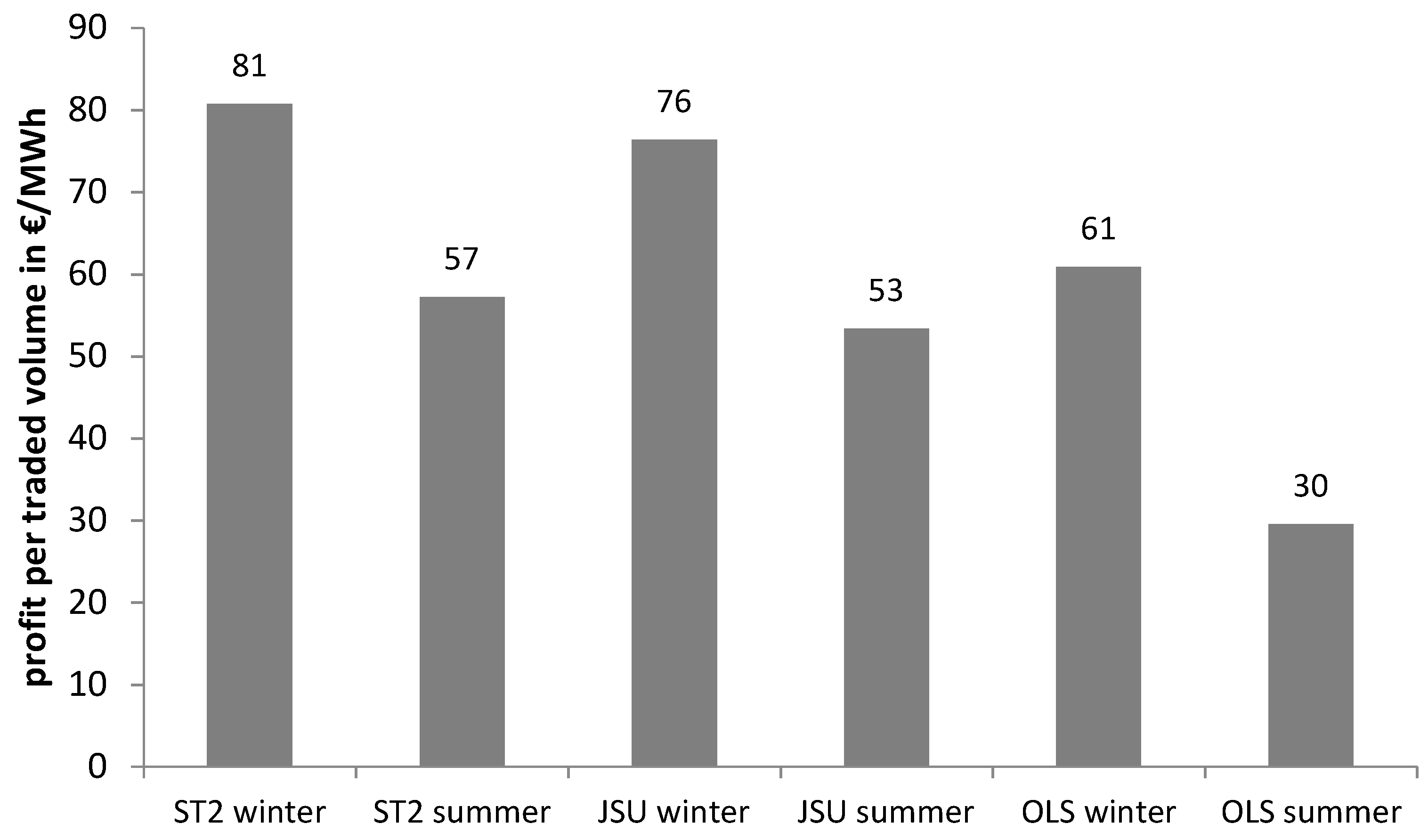
The out-of-sample backtests are evaluated by profit and risk parameters. Profit per traded MWh is shown in Figure 3 and indicates the average profitability per trade. Evidently, the density ST2 model increases profitability by about a third in winter and almost twice as much in summer. The JSU model outperforms the OLS as well but profits per traded MWh are slightly lower than the profits from the ST2 model.

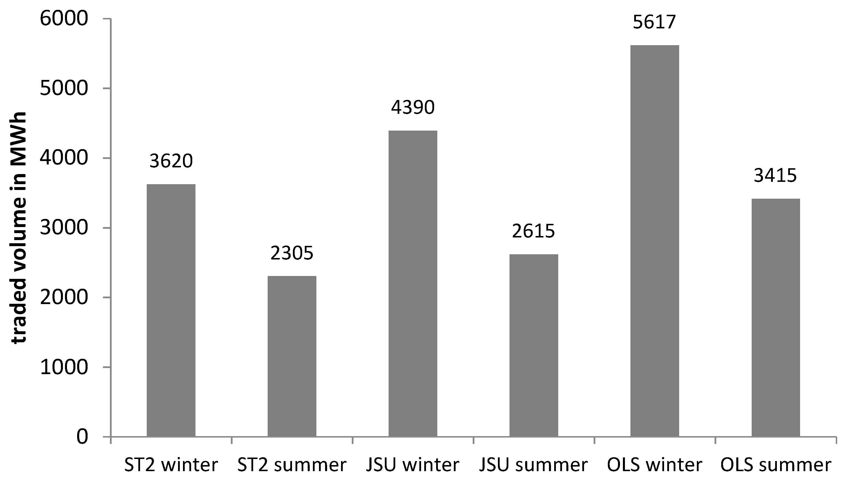
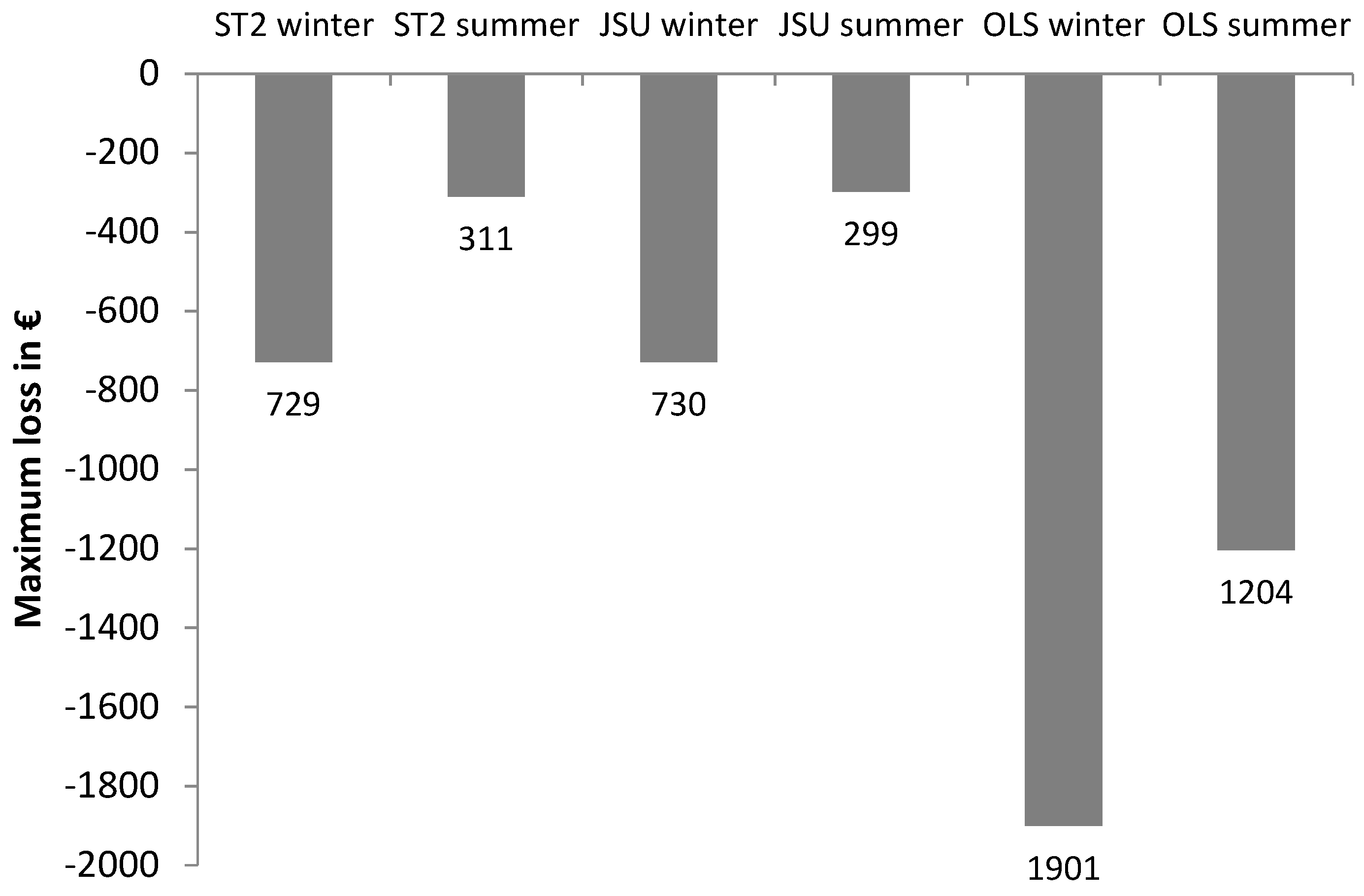
Traded volume (Figure 4) was significantly higher for the OLS model. The OLS model traded 5617 (3415) MWh in winter (summer) compared to 3620 (2305) MWh traded by the ST2 model and 4390 (2615) by the JSU model. Evidently, the density function predictor caused the traders to be more selective compared to mean value (OLS), and this is further demonstrated in Figure 5, where the maximum losses for the OLS are much higher, as well.

The same analysis was also undertaken using the JSU distribution instead of the ST2. Although Figure 2 indicated that the JSU fitted rather better in-sample, undertaking the full predictive modeling and backtesting revealed less attractive performance out-of-sample. Figure 6 shows the observed imbalance (without trading) and compares it with the backtested imbalance from the ST2, JSU and OLS model in 15 min resolution. The OLS-based decision rule shows higher trading volumes. This causes more frequent overreactions and imbalance sign flips in the backtest. For example, at 5:30 on the 20th February 2015, the OLS model caused a sign flip from −16 MWh in the observed data to +11 MWh (a trading volume of 27 MWh), which led to losses due to the single price system. The ST2/JSU model traded only 8/12 MWh (from −16 MWh to −8/−4 MWh) and was therefore still profitable.

For profitability, in winter the JSU backtest gave 76.37 €/MWh, compared to 80.77 €/MWh for ST2, and in summer it gave 53.38 €/MWh compared to 57.24 €/MWh. This out-of-sample performance is consistent with the comparison between skew-t and JSU for day ahead German hourly price predictions in [6].

6. Conclusions

It has been demonstrated that using a density function predictor as a basis for trading imbalances on the Austrian electricity market can be much more profitable and financially less risky than relying upon mean value, regression-based estimates. This evaluation was based upon detailed out-of-sample backtesting and is one of the few examples to assess forecasting within realistic decision-making processes. Trading with the ST2 density model was 33% more profitable in winter and 94% more profitable in summer. This appeared to have been achieved by a more selective approach to trading, thereby limiting the maximum losses quite considerably. A risk-neutral, flexible generator has been assumed. Evidently, with risk aversion, the attraction of the density model would be even greater.

This research is also unusual in looking at forecasting the volume required to be managed by the system operator in a real-time balancing market. These results show that imbalance volumes are predictable by market participants acting on the Austrian market. The key predictive variables were lagged imbalances and forecast errors in load, wind and solar generation, made available to the market two periods beforehand. The analysis in this research is based upon incremental activities, and if it were to become more widespread, as with most arbitrage-based trading, the benefits would be reduced through greater participation.

Finally, this research provides further documentation of the stochastic latent moment approach to density forecasting in an electricity market context. By estimating the first three moments of a flexible density such as the skew-t, as linear functions of exogenous factors, the key driving factors can be modeled in a way that not only influences the expectation, but also the variance and skewness, so that the whole predictive density shape is driven by these factors. Estimating the first three moments in terms of factors is found to be sufficient, even though the skew-t is a four-parameter density. Finally, it can also be concluded that it is better to identify the most appropriate density function in the context of out-of-sample prediction and backtesting, rather than simply looking at in-sample fit to the empirical data.

References

- Nowotarski, J.; Weron, R. Recent advances in electricity price forecasting: A review of probabilistic forecasting. Renew. Sustain. Energy Rev. 2018, 81, 1548–1568. [Google Scholar] [CrossRef]
- Weron, R. Electricity price forecasting: A review of the state-of-the-art with a look into the future. Int. J. Forecast. 2014, 30, 1030–1081. [Google Scholar] [CrossRef]
- Jónsson, T.; Pinson, P.; Nielsen, H.A.; Madsen, H. Exponential smoothing approaches for prediction in real-time electricity markets. Energies 2014, 7, 3710–3732. [Google Scholar] [CrossRef] [Green Version]
- Bello, A.; Bunn, D.; Reneses, J.; Muñoz, A. Parametric Density Recalibration of a Fundamental Market Model to Forecast Electricity Prices. Energies 2016, 9. [Google Scholar] [CrossRef]
- Chan, J.C.C.; Grant, A.L. Modeling energy price dynamics: GARCH versus stochastic volatility. Energy Econ. 2016, 54, 182–189. [Google Scholar] [CrossRef] [Green Version]
- Jiang, P.; Liu, F.; Song, Y. A hybrid multi-step model for forecasting day-ahead electricity price based on optimization, fuzzy logic and model selection. Energies 2016, 9. [Google Scholar] [CrossRef]
- Uniejewski, B.; Weron, R.; Ziel, F. Variance Stabilizing Transformations for Electricity Spot Price Forecasting. IEEE Trans. Power Syst. 2018, 33, 2219–2229. [Google Scholar] [CrossRef]
- Hagfors, L.I.; Bunn, D.; Kristoffersen, E.; Staver, T.T.; Westgaard, S. Modeling the UK electricity price distributions using quantile regression. Energy 2016, 102, 231–243. [Google Scholar] [CrossRef]
- Lago, J.; De Ridder, F.; De Schutter, B. Forecasting spot electricity prices: Deep learning approaches and empirical comparison of traditional algorithms. Appl. Energy 2018, 221, 386–405. [Google Scholar] [CrossRef]
- Singh, S.; Yassine, A. Big Data Mining of Energy Time Series for Behavioral Analytics and Energy Consumption Forecasting. Energies 2018, 11, 452. [Google Scholar] [CrossRef]
- Gajowniczek, K.; Ząbkowski, T. Two-Stage Electricity Demand Modeling Using Machine Learning Algorithms. Energies 2017, 10, 1547. [Google Scholar] [CrossRef]
- Wang, H.-Z.; Li, G.-Q.; Wang, G.-B.; Peng, J.-C.; Jiang, H.; Liu, Y.-T. Deep learning based ensemble approach for probabilistic wind power forecasting. Appl. Energy 2017, 188, 56–70. [Google Scholar] [CrossRef]
- Yang, Z.; Ce, L.; Lian, L. Electricity price forecasting by a hybrid model, combining wavelet transform, ARMA and kernel-based extreme learning machine methods. Appl. Energy 2017, 190, 291–305. [Google Scholar] [CrossRef]
- Areekul, P.; Senjyu, T.; Toyama, H.; Yona, A. A hybrid ARIMA and neural network model for short-term price forecasting in deregulated market. IEEE Trans. Power Syst. 2010, 25, 524–530. [Google Scholar] [CrossRef]
- Maciejowska, K.; Nowotarski, J.; Weron, R. Probabilistic forecasting of electricity spot prices using Factor Quantile Regression Averaging. Int. J. Forecast. 2016, 32, 957–965. [Google Scholar] [CrossRef]
- Panagiotelis, A.; Smith, M. Bayesian density forecasting of intraday electricity prices using multivariate skew t distributions. Int. J. Forecast. 2008, 24, 710–727. [Google Scholar] [CrossRef]
- Serinaldi, F. Distributional modeling and short-term forecasting of electricity prices by Generalized Additive Models for Location, Scale and Shape. Energy Econ. 2011, 33, 1216–1226. [Google Scholar] [CrossRef]
- Gianfreda, A.; Bunn, D. A Stochastic Latent Moment Model for Electricity Price Formation. Oper. Res. Forthcom. 2018. [Google Scholar] [CrossRef]
- Gianfreda, A.; Ravazzolo, F.; Rossini, L. Comparing the Forecasting Performances of Linear Models for Electricity Prices with High RES Penetration. arXiv, 2018; arXiv:1801.01093. [Google Scholar]
- Kupiec, P.H. Techniques for Verifying the Accuracy of Risk Measurement Models. J. Deriv. Winter 1995, 3, 73–84. [Google Scholar] [CrossRef]
- Christoffersen, P. Evaluating Interval Forecasts. Int. Econ. Rev. (Phila.) 1998, 39, 841–862. [Google Scholar] [CrossRef]
- Hong, T.; Pinson, P.; Fan, S.; Zareipour, H.; Troccoli, A.; Hyndman, R.J. Probabilistic energy forecasting: Global Energy Forecasting Competition 2014 and beyond. Int. J. Forecast. 2016, 32, 896–913. [Google Scholar] [CrossRef] [Green Version]
- Kraas, B.; Schroedter-Homscheidt, M.; Madlener, R. Economic merits of a state-of-the-art concentrating solar power forecasting system for participation in the Spanish electricity market. Sol. Energy 2013, 93, 244–255. [Google Scholar] [CrossRef]
- Barthelmie, R.J.; Murray, F.; Pryor, S.C. The economic benefit of short-term forecasting for wind energy in the UK electricity market. Energy Policy 2008, 36, 1687–1696. [Google Scholar] [CrossRef]
- Zareipour, H.; Canizares, C.A.; Bhattacharya, K. Economic Impact of Electricity Market Price Forecasting Errors: A Demand-Side Analysis. IEEE Trans. Power Syst. 2010, 25, 254–262. [Google Scholar] [CrossRef]
- Bunn, D.W.; Kermer, S. Statistical Arbitrage and Information Flow in an Electricity Balancing Market. SSRN Electron. J. 2018. [Google Scholar] [CrossRef]
- Johnson, N.L. Systems of frequency curves derived from the first law of Laplace. Trab. Estad. 1954, 5, 283–291. [Google Scholar] [CrossRef]
- Jones, M.C.; Pewsey, A. Sinh-arcsinh distributions. Biometrika 2009, 96, 761–780. [Google Scholar] [CrossRef] [Green Version]
- Azzalini, A.; Capitanio, A. Distributions generated by perturbation of symmetry with emphasis on a multivariate skew t-distribution. J. R. Stat. Soc. Ser. B Stat. Methodol. 2003, 65, 367–389. [Google Scholar] [CrossRef] [Green Version]
- Jones, M.C.; Faddy, M. A skew extension of the t-distribution, with applications. J. R. Stat. Soc. Ser. B Stat. Methodol. 2003, 65, 159–174. [Google Scholar] [CrossRef]
- Azzalini, A. Further results on a class of distributions which includes the normal ones. Statistica 1986, 46, 1973–2201. [Google Scholar]
- Ziel, F.; Weron, R. Day-ahead electricity price forecasting with high-dimensional structures: Univariate vs. multivariate modeling frameworks. Energy Econ. 2018, 70, 396–420. [Google Scholar] [CrossRef] [Green Version]
- Weber, C.; Just, S. Strategic Behavior in the German Balancing Energy Mechanism: Incentives, Evidence, Costs and Solutions. J. Regul. Econ. 2012, 48. [Google Scholar] [CrossRef]
- Ding, H.; Pinson, P.; Hu, Z.; Wang, J.; Song, Y. Optimal Offering and Operating Strategy for a Large Wind-Storage System as a Price Maker. IEEE Trans. Power Syst. 2017, 32, 4904–4913. [Google Scholar] [CrossRef]
- Krishnamurthy, D.; Uckun, C.; Zhou, Z.; Thimmapuram, P.R.; Botterud, A. Energy Storage Arbitrage Under Day-Ahead and Real-Time Price Uncertainty. IEEE Trans. Power Syst. 2018, 33, 84–93. [Google Scholar] [CrossRef]
- Browell, J. Risk Constrained Trading Strategies for Stochastic Generation with a Single-Price Balancing Market. Energies 2018, 11. [Google Scholar] [CrossRef]
- Pinson, P.; Chevallier, C.; Kariniotakis, G.N. Trading wind generation from short-term probabilistic forecasts of wind power. IEEE Trans. Power Syst. 2007, 22, 1148–1156. [Google Scholar] [CrossRef] [Green Version]
Figure 1.
Balancing price formation (source: APCS, 2018, [26]).
Figure 2.
Comparisons of density fits for JSU, ST, SN and NO distributions.
Figure 3.
Profit per traded MWh.
Figure 4.
Traded volume.
Figure 5.
Maximum loss.
Figure 6.
Illustrative imbalances with/without trading in backtesting.