Identification of Power Transformer Winding Fault Types by a Hierarchical Dimension Reduction Classifier


1
Department of Electrical Engineering, Tsinghua University, Beijing 100084, China
2
Sichuan Energy Internet Research Institute, Tsinghua University, Chengdu 610213, China
3
Swatow Power Supply Bureau, Guangdong Power Grid Co., Ltd., Swatow 515000, China
*
Author to whom correspondence should be addressed.
Energies 2018, 11(9), 2434; https://doi.org/10.3390/en11092434
Submission received: 21 August 2018
/
Revised: 7 September 2018
/
Accepted: 7 September 2018
/
Published: 14 September 2018
(This article belongs to the Section F: Electrical Engineering)
Abstract
:Frequency response analysis (FRA) demonstrates significant advantages in the diagnosis of transformer winding faults. The instrument market desires intelligent diagnostic functions to ensure that the FRA technique is more practically useful. In this paper, a hierarchical dimension reduction (HDR) classifier is proposed to identify types of typical incipient winding faults. The classifier procedure is hierarchical. First, measured frequency response (FR) curves are preprocessed using binarization and binary erosion to normalize FR data. Second, the pre-processed data are divided into groups according to the definition of dynamic frequency sub-bands. Then, hybrid algorithms comprised of two conventional and two novel quantitative indices are used to reduce the dimension of the FR data and extract the features for identifying typical types of transformer winding faults. The classifier provides an integration of a priori expertise and quantitative analysis in the furtherance of the automatic identification of FR data. Twenty-six sets of FR data from different types of power transformers with multiple types of winding faults were collected from an experimental simulation, literature, and real tests performed by a grid company. Finally, real case studies were conducted to verify the performance of the HDR classifier in the automatic identification of transformer winding faults.
1. Introduction
Power transformers provide indispensable services for the transmission and distribution of electrical power. Failures of in-service power transformers not only impair the system’s performance, but also have a serious social impact because of unscheduled outages of the electricity supply [1,2]. Consequently, advanced diagnostic methods for detecting transformer faults are becoming vitally important for maintenance work.
Many monitoring and diagnostic technologies have been developed to address the problems in transformers. Online monitoring technologies can provide real-time information of the power equipment’s state [3]. Nowadays, the key operation parameters of power transformers such as terminal voltage, current, ampere turns, and temperature are usually monitored continuously. These monitoring data are used in the transformer protection zone for real-time state estimation [4,5]. Besides, there is a growing trend to develop the dissolved gas analysis (DGA) as an online monitoring measurement for detecting the incipient fault of power transformers [6,7]. Several intelligent machine learning approaches, such as genetic algorithm, the neuro-fuzzy inference system, and vector support machine have been used to analyze the DGA results [6,7]. However, some types of internal faults of power transformers are undetectable by these online monitoring and diagnostic methods. According to a statement in [8], statistics show that 70% to 80% of failure regarding power transformers are caused by undetected winding faults. Commonly used approaches for detecting incipient winding faults are usually offline tests, such as the short-circuit impedance measurement (SCI) [9], low-voltage impulse tests (LVI) [10], and frequency response analysis (FRA) [11,12,13,14,15].
Among the existing test approaches, FRA is a well-recognized technique for diagnosing incipient winding faults in power transformers [11,12,13,14,15]. Depending on the types of injected signals, there are two major types of FRA, which are the sweep frequency response analysis (SFRA) and impulse frequency response analysis (IFRA) [8]. The injected signal of SFRA is a sinuous wave, and the response signal is measured in the frequency domain. For IFRA, an impulse wave with a wideband frequency spectrum is injected as the input, and the output is measured in the time domain. Then, the frequency response (FR) is derived by converting the results to a frequency domain [16]. Based on the comparing the studies in [8,15], the results and sensitivities of SFRA and IFRA are similar for detecting faults in the short circuit. However, in some literature [17], it states that IFRA could encounter drawbacks of low resolution in low frequencies. In recent years, online FRA has been studied by some researchers [18,19], and online FRA measurements in the low-frequency range has been found to be easily affected by external disturbances. This online technology has not been applied in real in-service power transformers and is also not widely accepted by the industry. Because the analysis in this paper is based on offline SFRA, for convenience of description, the FRA mentioned below represents SFRA.
The faults (or ‘failure modes’) of windings are typically caused by a mechanical change or electrical change inside the transformer. Mechanical changes, including radial bulking, axial displacement, tilting, and hoop tension arise for many reasons, such as electromagnetic force induced by a short-circuit current, improper transportation, and damage from a natural outside force [20,21,22,23]. This type of fault in transformer winding is difficult to perceive because of the imperceptible impact on the normal operation of power transformers. Electrical changes, such as short-circuited turns (SCT) and open-circuited turns (OCT), are typically caused by aging of the insulation layer and the explosion of combustible gas in oil [24]. SCT and OCT lead to different deteriorative consequences, and the FRA results of these two types of faults can be used to confirm the results of other diagnostic tests, such as direct-current winding resistance. These failure modes are not necessarily a real failure, but they degrade the ability to withstand short-circuit current and overvoltage, thereby eventually leading to solid failure. Thus, as an outstanding technique for the diagnosis of windings, academic institutions have recommended that the offline FRA test is performed on new transformers and as a standard procedure of subsequent routine tests [12,24].
However, FR diagnosis requires engineers to have experiential knowledge of the FRA test [12,24]. With regard to this, most recent FRA measurement instruments typically contain computer-aided software to automatically diagnose the transformer conditions [10]. The software uses a certain index to quantitatively analyze the FRA results. A variety of indices have been proposed for quantitative FRA interpretation, such as the correlation coefficient (CC), spectrum deviation (σ or SD), and absolute sum of logarithmic error (ASLE) [23,24,25,26,27,28,29]. However, the sensitivity of each index differs with respect to different morphological characteristics of the deviation between two FR curves over the entire spectrum. For instance, CC is insensitive to the vertical displacement of curves. Because of a lack of effective methods to automatically identify types of transformer winding faults, the quantitative interpretation methods adopted in modern FRA measurement instruments only provide information on the severity of deformation at the current stage [30]. Despite this, identifying different faults that result in different consequences does not only provide information on preventive actions, but also supports a united diagnosis with other diagnostic tests. Therefore, the purpose of this paper is to propose a new automatic approach to identify three types of typical incipient winding faults (i.e., mechanical deformation (MD), SCT, and OCT) that require different further preventive and inspective actions.
Moreover, the indices involved in the typical quantitative methods are calculated either in the entire frequency range or by using fixed frequency sub-bands. In the mechanism research of FRA, the effects of different electrical parameters of power-transformer-equivalent circuits are perceptible in different frequency sub-bands [21,22,31]. As stated in [24], the described frequency regions are typical but not exact, and they vary slightly depending on the transformer’s design and arrangement. Hence, dynamically identifying the frequency sub-bands for every specific type of winding can provide a stronger connection between the quantitative results and the affected electrical parameters, thereby assisting the development of better interpretation tools for automatic diagnosis. Several methods that adapt frequency sub-bands for a specific winding have been proposed based on the zero crossing points in the phase plot of the FR [32,33]. However, according to a newly published discussion on the IEEE standard (C57.149-2012 [24]), the theory of the relations between the resonance and phase zero points claimed in [24] was misconstrued [34]. It claimed that, at resonance, the input impedance is not purely resistive and the phase angle between the input voltage and current is not always zero. Inevitably, the dynamic methods of dividing frequency sub-bands according to the doubtful theoretical basis in [32,33,35] are problematic. An improved approach, according to binary erosion and first anti-resonance, is adopted in this paper to divide the frequency sub-band dynamically. A similar method was proposed and validated in the authors’ previous research [36].
The remainder of the paper is organized as follows: To normalize FR curves measured from different types of power transformers, image processing technologies, including image binarization and binary erosion, are introduced and used in Section 2 as a preprocessing procedure. In Section 3, an approach is presented for the dynamic division of frequency sub-bands on the basis of the five suggested sub-bands. In Section 4, the experimental setup and data preparation are explained. In the following section, a new classifier, that is, the hierarchical dimension reduction (HDR) classifier, is proposed based on hybrid indices, including CC, SD, and two new types of indices. The purpose of this classifier is to identify three typical types of incipient winding faults that require different further preventive and inspective actions. Finally, in Section 5, real case studies are investigated to demonstrate the performance of the HDR classifier, followed by a conclusions section.
2. Preprocessing of Frequency Response Data
FR data are typically presented in the form of spectrum diagrams for visual evaluation by human experts. The most important part of interpreting FR data is to extract characteristic information from the frequency range where clean-cut deviations are shown. Considering an FRA diagram as an image with uniform size, image processing techniques can then be applied to manifest the deviations between curves in a normalized manner.
2.1. Theory of Binary Erosion
The main notion of mathematical morphology (MM) is to extract relevant structures in an image by probing the image with a simple shape called a structuring element (SE) [37]. Erosion is one of the basic operators of MM. The basic effect of the erosion operator on a binary image is to erode the boundaries of regions of foreground pixels (i.e., white pixels with intensity value ‘1′). This function matches the aforementioned objective of preprocessing FRA spectra. Hence, in the present work, binary erosion is used as a filter to identify the major areas where distinct deviations between ‘reference’ and ‘suspected response’ curves exist.
A binary image can be regarded as a set of pixels with two possible intensity values (i.e., ‘0′ and ‘1′). A binary image is denoted as ‘A’, with components a = (a1, a2), where a1 and a2 represent the pixel locations. An SE is regarded as ‘B’, with components b = (b1, b2). The shape of the SE is pre-defined according to some a priori knowledge about the shape of the image. Then, the erosion of binary image A by SE B can be mathematically defined as:
where ⊖ is the erosion operator.
2.2. Binarization of the Frequency Response Spectrum
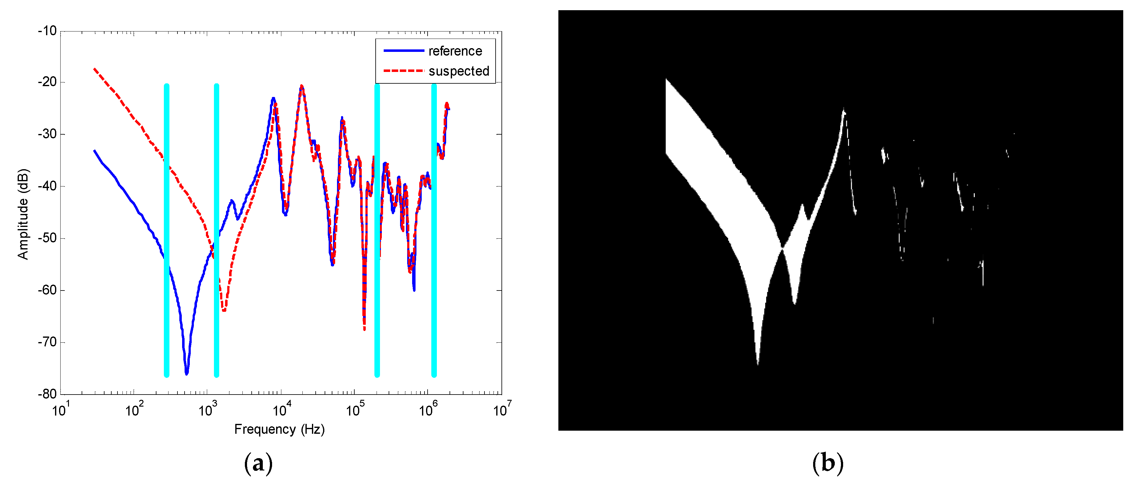
The original FR data are a set of discrete data points organized by frequency. To apply the operation of binary erosion, the input data have to be transformed into a digital binary image of a uniform size. Typically, the FR spectrum is presented in different types of diagrams using linear or logarithmic scales for the abscissa and ordinate for visual evaluation. The selection of the type depends on which range of magnitude or frequency is of special interest. Double logarithmic scales are appropriate for obtaining an overview of the FR spectrum. This type of diagram is the most frequently used form in FRA interpretation, as, for example, in Figure 1. All the FR data used in this work appear as magnitude () versus frequency () spectra with double logarithmic scales and are denoted as . The intensity of the pixels between the two curves is set as the value ‘1,’ which means white. Other pixels are set to be ‘0,’ which means black. For instance, Figure 1b depicts the binary image of Figure 1a after conversion, in which all areas with deviations are highlighted.
The relation between the binary image and FR spectrum is derived using the reference curve. In the FR spectrum, the reference is denoted by , and in the digital image, the reference is denoted by The location of pixels in the binary image is represented by (). The relations between these two forms of coordinates are thus expressed as:
where [] represents the rounding operator and N is the total number of reference points.
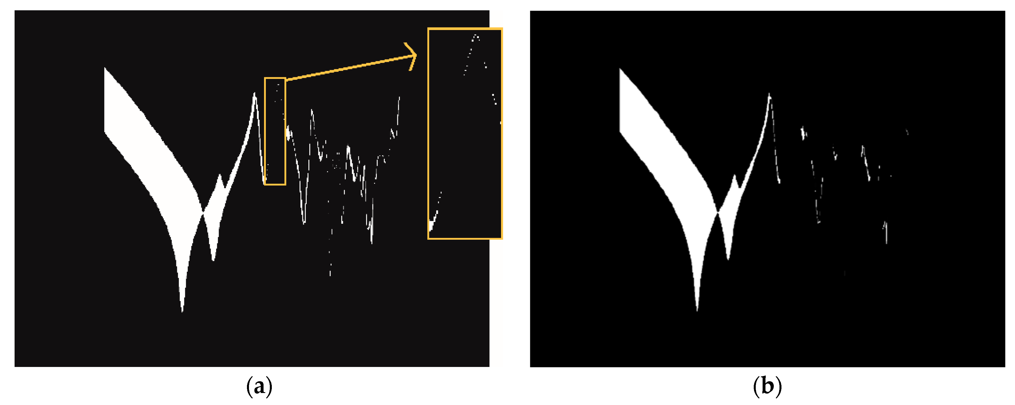
Some minor deviations that probably arise from admissible measurement errors are negligible, as shown in Figure 2a. The calculated results of the pertinent statistical indices, such as CC, can become more responsive when they are calculated without considering the data that corresponds to admissible measurement errors, which agrees with visual-based judgment. Hence, erosion is applied in the next step to filter the areas with minor deviations.
2.3. Application of Erosion
In the binary images, as each frequency point corresponds to a white rectangle (deviation area) or nothing (no deviation), a rectangular SE was used for erosion in this case. The size of the SE is considered as a threshold value to determine how large an area should be dismissed, and the size of the rectangular SE is defined by the following equation in this application:
where ‘[]’ represents the rounding operator, k is a constant coefficient, H is the maximum difference of vertical pixel positions on the curves, and W is the width of the rectangular SE. [k × H], which is the height of the SE, is adaptable to each FR diagram with different degrees of deviation. According to the result proved in [36], k and W are set to ‘0.01′ and ‘2,’ respectively.
Figure 2b shows an example of an eroded image, where the SE defined in Equation (2) is used to erode the binary image shown in Figure 2a. It can be found that most of the thin areas that indicated minor deviations were removed. The retained segments after erosion correspond to the frequency ranges, with major deviations between the two curves.
3. Dynamic Division of Frequency Sub-Bands
Relevant international standards recommend that the frequency range of the FRA test shall be 20 Hz to 2 MHz, at the least [33]. As mentioned previously, calculating indices in divided frequency regions can increase sensitivity to winding faults, because the effects of the equivalent electrical parameters are reflected in different frequency bands. A generalized sub-band structure of frequency boundaries is illustrated in Figure 3. Another fact is that the patterns of FR to each specific transformer can vary according to its design and interconnections [11]. The characterization of typical FR patterns was conducted in [11], demonstrating that the boundaries of frequency sub-bands cannot be found explicitly. To adapt the frequency sub-bands to each specific FR, an improved and uncomplicated approach is adopted in this section. This approach is based on the sub-band structure and careful analysis of the FR patterns of multiform transformers. The algorithms illustrated in Figure 4 provide the procedure that divides the frequency range into five sub-bands specifically for each case of FR curves. The explanation of the procedure is listed in detail as follows.
- In LF1 shown as Figure 3, the key feature of the FR curves is that they typically begin with an almost linearly decreasing magnitude of 20 dB/decade because of the magnetizing inductance (Lm) of the core [24]. For some connection configurations, they are typically smooth and dominated by the total inductance. This is then followed by a minimum, which is the key feature in sub-band LF2. This minimum resonance, marked as Zm, occurs because of the series resonance between Lm and shunt capacitance (Cg). Hence, the boundaries B and C should satisfy the conditions that the potential linear part is located in LF1, and the minimum remains in LF2. Through the analysis of a variety of FR curves, the boundaries B and C can be determined using the left flowchart illustrated in Figure 4. The essential strategy is to locate the minimum point Zm. Typically, Zm is the minimum point of the entire curve, but for some middle-voltage (MV) or low-voltage (LV) windings, drastic oscillations can occur at high frequencies. To eliminate the errors caused by these points, only the first three valleys are compared, without counting the valleys at comparatively higher frequencies according to the experience of FR patterns of power transformers. After locating Zm, the peak next to point Zm (marked as Pm) can be located to define the upper boundary of LF2. Thus, following the algorithms in the left flowchart, the boundaries A, B, and C are defined.
- The FR patterns in middle frequency (MF) sub-band typically present multiple oscillations in this range. The subsequent high-frequency (HF1) spectrum is often known to have a rising trend with damped oscillations typically because of high series capacitance (Cs) compared with Cg. However, for MV or LV windings, Cs is not required to be much higher than Cg in design. The FR patterns of these types of windings in HF1 do not demonstrate a capacitive rising trend. Consequently, boundaries D and E are difficult to determine. For this reason, a compromise between the representation of more general FR patterns and dynamic features for each specific case is reached to determine the boundaries D and E in this strategy.
The definition of boundaries D and E is based on the typical fixed values (illustrated in Figure 3) and information in the retained segments after erosion. This procedure attempts to avoid the separation of a continuous white area near the fixed frequency boundaries D and E, because in most cases, deviations in the nearby areas in the FR patterns typically arise from a chain effect of the same electrical component. If the section with these deviations is separated into two sub-bands, then the sensitivity of the calculated statistical indices could be adversely affected. The strategic algorithms to identify D and E are shown by the flowchart on the right in Figure 4, where k is the abscissa of the pixel. The corresponding frequency value f(k) can be derived using Equation (2). The basic idea is to search for a break column, where all the pixels in this column are black from right to left in a predefined range of frequencies around the fixed boundary.
To summarize, the algorithms illustrated in Figure 4 provide a method that divides the frequency range into five sub-bands specifically for each case of FR. This method is based on the authors’ previous work in [36], with a slight improvement. The performance of this approach was proven in [36], so it will not be repeated in this article.
4. Experimental Setup and Data Preparation
4.1. Experimenatal Setup
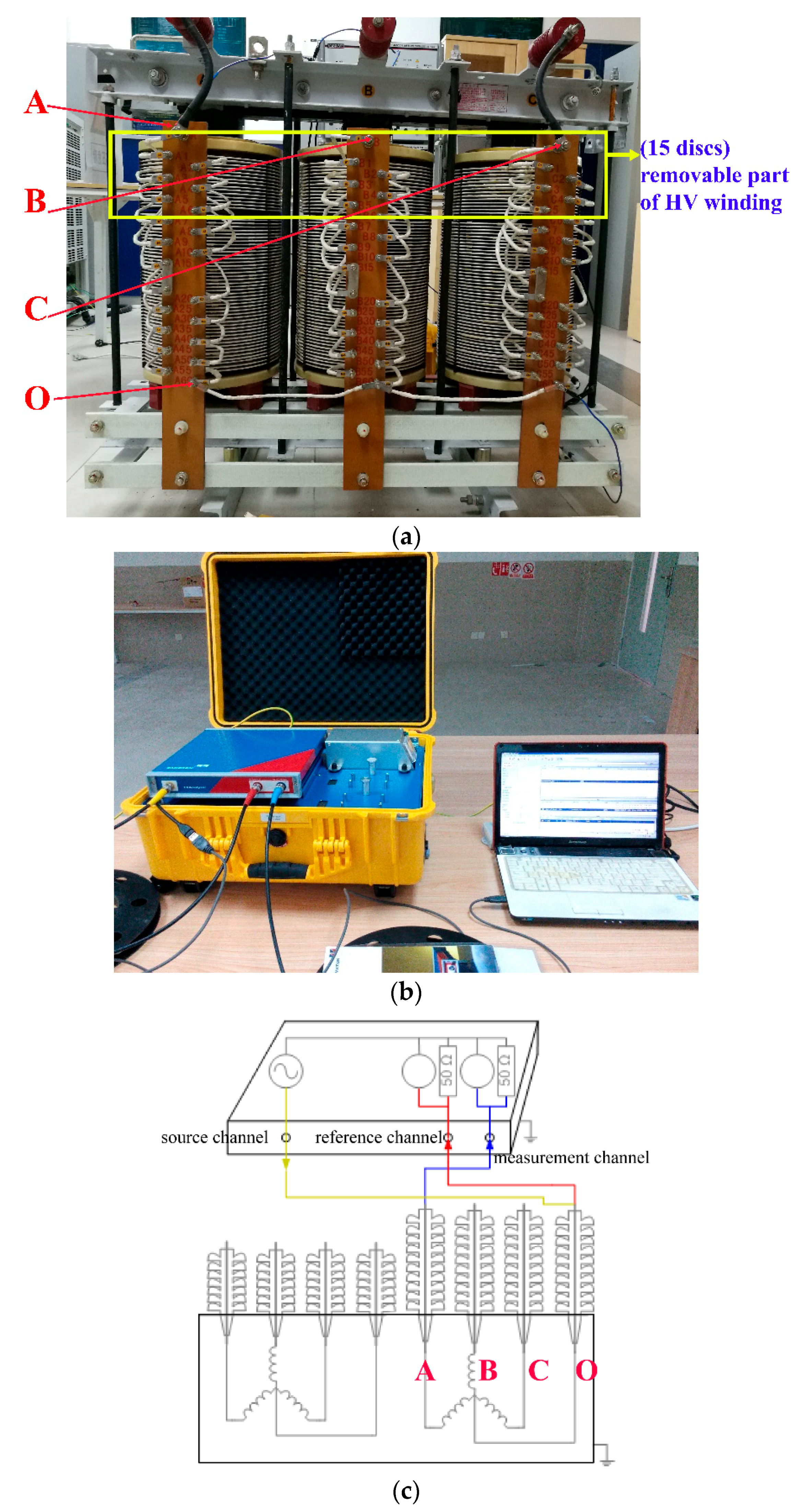
In this paper, a part of the training data was collected from a simulation experiment of typical cases of MD. A 50 kVA (10/0.4) kV three-phase power transformer was customized for the experiment. As shown in Figure 5a, the high-voltage (HV) winding of this power transformer contained sixty discs, where every disc consists of 15 turns of coils. Among these discs, 15 discs counting from the top in each phase are designated as movable and replaceable sections.
The sweep frequency response measurement was carried out by using a sweep frequency response analyzer, which is shown is Figure 5b. The connection method in this measurement adopts the end-to-end open-circuit method, illustrated in Figure 5c. The connecting terminals A, B, C, and O in the schematic diagram correspond to the marks in Figure 5a. A sinusoidal signal was injected from the source channel to the terminal O, and this input signal was recorded by the reference channel. Meanwhile, the output signal was measured from anther terminal (A, B, or C) by the measurement channel. Other untested terminals were floating. Consequently, the frequency response was derived by the ratio between the output and the input.
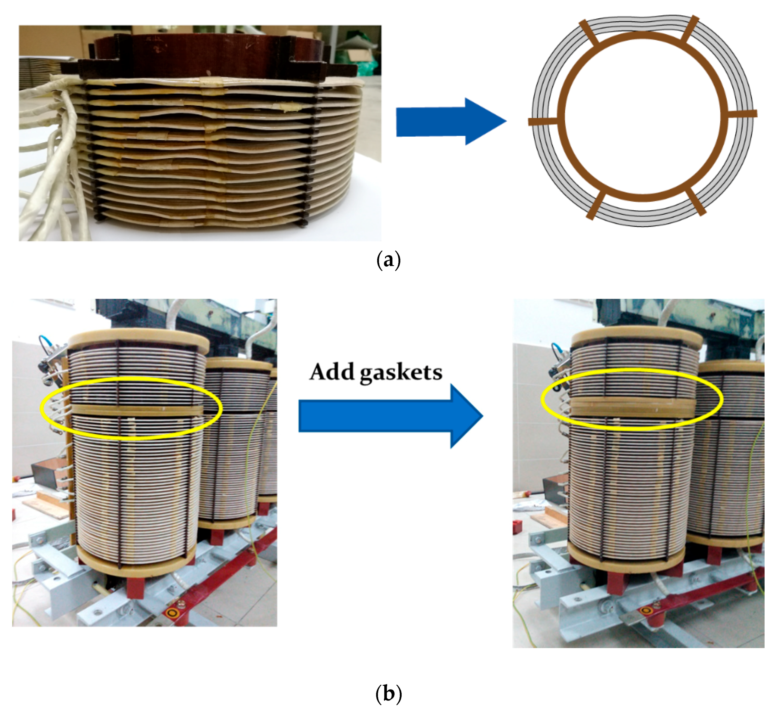
Cases of MD are simulated in the experiment. A typical case of radial buckling is arranged by replacing the removable part of the winding by a winding with buckling on the discs, shown in Figure 6a. The number of buckling in different directions represents different severity of the deformation. On the other hand, in order to arrange an experiment of localized axial winding displacement, a certain number of gaskets were added between the removable and fixed sections of the winding to move the top section of 15 discs upwards, which is demonstrated in Figure 6b. More numbers of gaskets mean greater severity of the displacement.
Four sets of data were obtained by the simulation of radial deformation, and five sets of data were collected from the simulation of the axial displacement. Figure 7 shows the examples of the FR curves from two cases of MD, respectively.
4.2. Preparation of Training Data
As mentioned, the purpose of this work was to propose an automatic approach to identify three typical types of incipient winding faults: MD, SCT, and OCT—reason being because these three types of winding faults have a similar symptom at an early stage but result in different consequences when they are aggravated. Hence, technology for the automatic identification of these faults can support preventive maintenance for power transformers.
Therefore, including the healthy condition of windings, four classes of FR curves were considered for automatic identification. Nevertheless, there were two scenarios for the healthy condition that needed to be considered. One was that the reference and suspected FR curves were consistent (this scenario of healthy condition is denoted by HC), and the other was that the two FRA measurements existed in different magnetic conditions (this scenario of different magnetic condition is denoted by DMC). For instance, there is residual magnetism in the measurements, or two compared curves were measured from the middle and side phases of a three-phase transformer, such as the reference curves in Figure 7a,b, respectively. DMC is not a fault, but this condition affects the FR curves, which could easily lead to misinterpretation. Hence, four types of conditions with five classes were considered, including DMC.
According to the prior knowledge summarized in [11,24,33,38], Table 1 highlights the characteristically affected sub-bands of each class. Logic ‘OR’ means that the affected frequency sub-bands could be any one of the marked sub-bands, and logic ‘AND’ means that this condition affects all marked sub-bands.
To define the threshold values of the applied indices, four sets of the experimental FR data were selected to be the training sets, which corresponded to the case of radial buckling, axial displacement, healthy winding tested from the same phase, and healthy winding tested from the middle phase and side phase. Among them, the case of one gasket and the case one buckling were used because they had the slightest severity of MD in the simulation. To ensure the capability of the proposed classifier for more general types of power transformers, in addition to the four sets of experimental data, 22 sets of FR data from different types of power transformers were also used as training sets. These 22 sets of data were collected from FRA tests of in-service power transformers performed by the China Southern Power Grid and analyzed cases in the published literature. Therefore, 26 sets of typical measured FR data were used for training the threshold values. Although the population of the datasets was not particularly large, the collected data represented a satisfactory amount of very typical cases of failure modes or conditions, and they were able to provide general threshold values. In future works, the threshold values can be refined using a larger number of training sets to consider more types of transformers.
5. Hierarchical Dimension Reduction Classifier
5.1. Indices for the Hierarchical Dimension Reduction Classifier
Before introducing the classifier, several statistical indices applied in the classifier need to be explained first. As mentioned in Section 1, the sensitivity of a single type of index is different regarding different morphological characteristics of the deviation between curves. Therefore, instead of using a single type of index for quantification, hybrid indices for different frequency sub-bands are designed to be used in the classifier. Among the statistical indices, CC is frequently used to evaluate the similarity between two sets of data, and SD is a normalization equation to measure the deviation between two sets of data. Their equations are expressed as:
where vectors X = {x1, x2, …, xN} and Y = {y1, y2, …, yN} denote two compared sets of data.
As explained in Section 3, the FR curve in LF1 is typically linear or smooth, so the common deviation of the FR curves in sub-band LF1 is vertical displacement. This type of characteristic deviation typically occurs when a winding being tested is in DMC, or when an electrical fault appears that affects the resistance and Lm of the test winding. CC is not sensitive to vertical changes. Although SD can detect this type of deviation, the calculated value of SD cannot detect the severity of the deviation explicitly. Moreover, the calculations of SD and CC do not have the ability to distinguish whether the curve is shifting upward or downward with reference to the reference curve. The shifting direction (upward or downward) in sub-band LF1 also contains vital information for identification. To overcome the weakness of SD and CC in LF1, two indices for evaluating the deviation in the low-frequency sub-bands are proposed—the area ratio index (ARI) and angle difference (AD)—which are defined in the following Equations (7) and (8).
ARI is designed to differentiate the shifting directions of curves and reflect the severity of the vertical deviation in a quantitative manner. The definition of ARI is expressed as:
where X = {x1, x2, …, xN} and Y = {y1, y2, …, yN} denotes the vertical pixel positions (py) of the two FR curves, and N is the number of pixels in the horizontal axis that corresponds to the maximum frequency point.
The explanation of ARI is illustrated in Figure 8a. The absolute value of ARI is equivalent to the area ratio of the deviation area in LF1 (yellow area) to the accumulated maximum area (dotted area). In most FR curves of power transformers, the slope angle is similar and does not change substantially. Therefore, the area ratio can reflect the severity of the deviation. The interval of ARI is [−1,1]. The sign of ARI represents the shifting direction of the suspected curve when compared with the reference curve. Considering X as a reference, a positive sign means that suspected curve Y moves below X (shifting downward), and a negative sign means that suspected curve Y moves above X (shifting upward). Therefore, the information about the shifting direction and severity of the deviation in sub-band LF1 is described by ARI.
The angle difference (AD) of the anti-resonance in LF2 (Zm, as explained in Section 3) is deliberately designed for coherent use with ARI. The definition of ARI is expressed as:
where atan2d{B, A} represents a function of a four-quadrant inverse tangent in degrees, as explained in Figure 8b. X(a1, b1) represents the pixel position of Zm in the reference curve, and Y(a2, b2) represents the pixel position of Zm in the suspected curve. The range of AD is (−180°, +180°].
ARI reflects the change of electrical parameters, which could be Lm or winding resistance. AD indicates the change of parameters, which could be Lm or Cg. Using them together, the changed electrical parameter can be distinguished from others, thereby substantially increasing the sensitivity of the hybrid indices in low-frequency ranges.
5.2. Hierarchical Dimension Reduction Classifier Algorithms
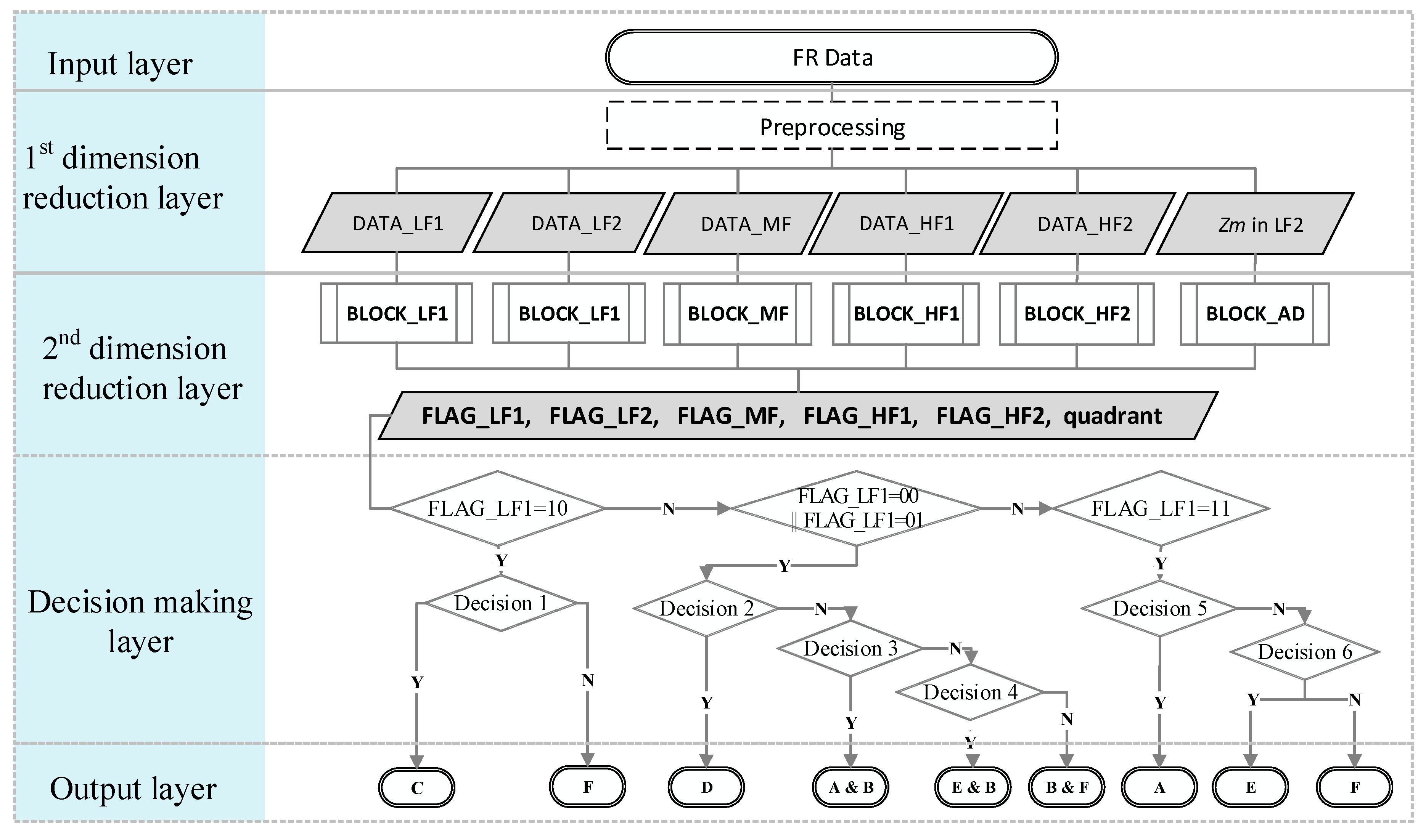
A set of FR data contains hundreds of values in a wide frequency range, which can be considered as a set of data with high-dimensional elements. The HDR classifier is designed to reduce the dimension and extract the key features from FR data so that the characteristics of different types of transformer winding faults can be identified automatically. The structure of the HDR classifier is explained in this subsection. A general flowchart describing the procedure of the HDR classifier is shown in Figure 9.
There are five layers of the HDR classifier. The structure is described as follows:
- (1)
- (2)
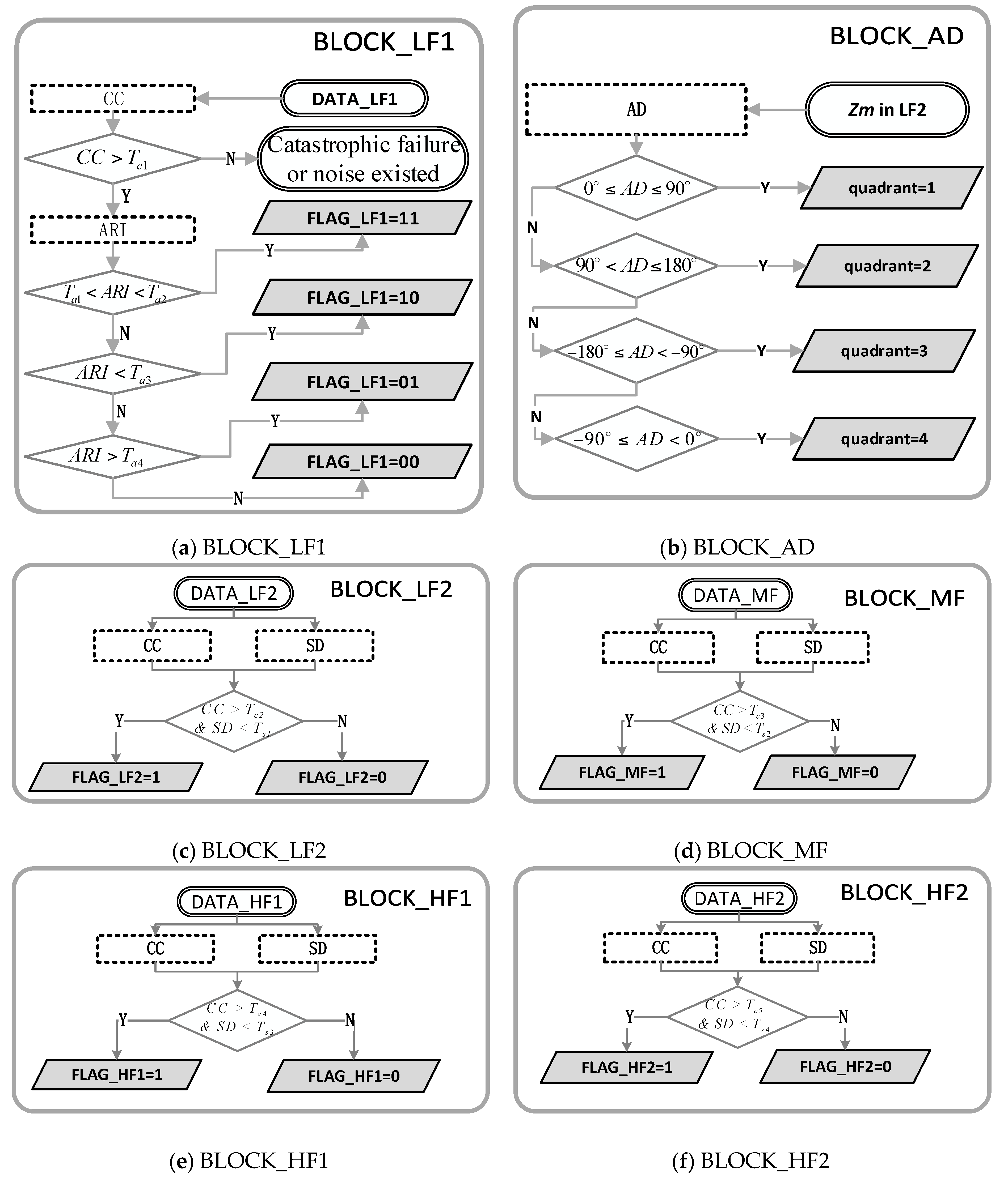
- In the 2nd dimension reduction layer, hybrid indices are used to reduce the dimensions of the grouped data into one dimension. The algorithms for each processing block are listed in Figure 10. The threshold values of the applied indices (Tc1, Ta1, Ts1, etc.) are determined using the 26 sets of training data that were described in Section 4. According to the training data, the threshold values are assigned as: Tc = [0.99, 0.998, 0.998, 0.995, 0.9920], Ta = [−0.1, 0.1, −0.5, 0.1], Ts = [0.04, 0.05, 0.07, 0.14]. As discussed previously, the threshold values can be refined if a larger number of training sets from more types of transformers can be collected.
BLOCK_LF1, depicted in Figure 10, involves the calculation of CC and ARI. As mentioned previously, CC is insensitive to vertical changes, so CC is first used to detect the cases in which catastrophic failure happens or the case in which some sharp noise is not filtered during the test. If the scenario is not found, then ARI is used to identify the shifting direction and severity of the vertical deviation in sub-band LF1, and the information is classified into four scenarios and recorded by FLAG_LF1.
In the algorithms for BLOCK_LF2, BLOCK_MF, BLOCK_HF1, and BLOCK_HF2, CC and SD are used together to assess the deviation in every sub-band because of their complementary sensitivities for different morphological characteristics of the deviation between curves. For the 1-bit binary output of every block, ‘1′ indicates significant deviation in a corresponding sub-band, and ‘0′ indicates negligible deviation in a corresponding sub-band. BLOCK_AD classifies the calculated AD into four classes, which indicate the located quadrants of the changed Zm. In short, the 2nd dimension reduction layer extracts the expected information from high-dimensional data groups into six dimensions.
- (3)
- The six-dimensional output from the last layer contains the features of the deviation between the FR curves. The decision-making layer uses the extracted features to identify the condition of the transformer winding. The decisions in this layer are based on the analyzed knowledge of typical winding faults that are summarized in Table 1. Different types of winding faults affect different equivalent parameters. Besides, these decisions are validated by using all training sets.
The output of the classifier is presented in Table 2. From Figure 9, it can be noticed that there exist outputs with combined classes, such as ‘E&B,’ which means mechanical deformation with a different magnetism condition. However, considering the real scenario of winding faults, some combinations, such as mechanical deformation with SCT or more complicated winding faults, are out of place at the current stage. Therefore, a class of ‘undetectable condition’ was added to remind the engineer that a more specific check is required.
In short summary, the HDR classifier processes input data in three layers. After the first- and second-dimension reduction layers, the input with hundreds of elements was reduced to 6 elements, which represent key features of the compared FR curves. According to the characteristics of changing equivalent parameters of each type of winding fault in every frequency sub-band, the 6 elements determine to which class the input belongs.
6. Validation and Discussion
To validate the HDR classifier, the proposed HDR classifier was further verified by five real FR cases. Two cases are discussed below.
Case 1: The FR curves of Case 1 were collected from the routine tests of a 240 MVA power transformer in a 220 kV substation in Guangzhou. According to the visual diagnosis conducted by experts, the result shows no fault in the tested windings. Because the two measurements were taken in different phases of the MV winding, the FR curves show deviation in the low-frequency range. In other words, the FRA result of this transformer winding deduces its healthy but different magnetism condition. Figure 11a shows the FR curves with boundaries of frequency sub-bands, and Figure 11b illustrates its eroded binary image.
From Figure 11, it can be seen that the deviation is located in LF1 and LF2. The diagnosis result using the HDR classifier is shown is Table 3. FLAG_MF, FLAG_HF1, and FLAG_HF2 all equal to 1, which means there is no noticeable deviation. FLAG_LF1 = 01 represents downward displacement in LF1, and FLAG_LF2 = 0 represents noticeable deviation in LF2. The diagnosed class of Case 1 is ‘A&B’, which means a healthy condition in a different magnetism. This result coincides with the visual diagnosis. Moreover, the relation coefficient (Rxy) stated in the Chinese Standard [25] was also applied to diagnose the FR curves, and its result is illustrated in Table 3. This diagnosed result using Rxy shows the tested winding is normal. The results are consistent, but a more detailed condition was given by using the HDR classifier.
Case 2: The FR curves used in this case are reprinted from [11]. The data were collected from a 140 MVA, 220/69 kV autotransformer. According to [11], the abnormality of the FR curves was caused by SCT. Figure 12 shows parts of images obtained from the implementation of the HDR classifier, and Table 4 illustrates the diagnosed results using the HDR and Rxy, respectively. The final class of Case 2 is ‘C’, which represents SCT. It matches with the known condition. The diagnosed result using Rxy also shows that a slight deformation of fault occurs in the tested winding, but the fault type cannot be revealed by using this common method.
The failure mode in this case mainly affects the Lm and winding resistance, so the most visible effect exists in LF1 and LF2. The effect of DMC is also located in these sub-bands. The identification between these two cases depends on the proposed indices, ARI and AD. Therefore, the result also verifies the performance of ARI and AD.
It can be summarized from the above cases that the HDR classifier has the ability to automatically identify the fault types in transformer windings. However, there are also drawbacks of this approach. (1) Due to lack of training data that covers all possible abnormalities in FRA, some abnormalities are not considered in the proposal of the HDR classifier, such as the abnormality caused by the reproducibility issue; (2) the training set is not particularly large. Despite this, the proposed approach is still serviceable. In future works, a larger number of training sets that cover more types of transformer winding faults are expected to be used to refine the threshold values for more classes of conditions. Moreover, the HDR classifier is applicable in potential commercial use. By embedding the HDR classifier into the FRA instruments, an automatic condition assessment of transformers could be realized during FRA measurement.
7. Conclusions
A novel HDR classifier that automatically identifies types of typical transformer winding faults has been proposed in this paper. The input was processed in hierarchical layers. Image binarization and binary erosion was applied in the first layer to normalize the FR data and eliminate minor deviation between the suspected and reference curves. A dynamic frequency region division method was also defined to divide the input data into certain groups, so that the effect of each equivalent parameter of a transformer winding could be distinguished.
In the next processing layer, hybrid indices were used to reduce the dimension of the FR data. The idea of hybrid indices takes advantage of every employed index so as to detect all morphological characteristics of the deviation between curves. The indices ARI and AD were presented for the first time, and are verified with respect to increasing sensitivity in a low-frequency range.
As opposed to other common classifiers such as the support vector machine, this classifier is based on the theoretical analysis of transformer winding faults rather than purely data-driven analysis. This advantage reduces the strict requirement of a large number of training sets. The threshold values of the HDR classifier were obtained by using 26 sets of FR data collected from various types of power transformers. The performance of the HDR classifier was demonstrated by two case studies. This classifier could potentially be used in FRA instruments to support the maintenance schedule of power transformers.
Author Contributions
H.L. and Z.Z. designed the experiment. Z.Z. wrote the code and the manuscript. T.K. debugged the code. W.G. supervised the research and edited the manuscript.
Funding
This research was funded by Nation High-tech R&D program of China (2015AA050201).
Acknowledgments
The authors thank Guangzhou Power Supply Bureau Co., Ltd. for offering the test data.
Conflicts of Interest
The authors declare no conflict of interest.
Abbreviations
The following abbreviations are used in this manuscript:
| ASLE | Absolute Sum of Logarithmic Error |
| CC | Correlation Coefficient |
| DGA | Dissolved Gas Analysis |
| FR | Frequency Response |
| FRA | Frequency Response Analysis |
| HDR | Hierarchical Dimension Reduction |
| HV | High Voltage |
| IFRA | Impulse Frequency Response Analysis |
| LV | Low Voltage |
| LVI | Low-Voltage Impulse |
| MD | Mechanical Deformation |
| MM | Mathematical Morphology |
| MV | Middle Voltage |
| OCT | Open-Circuited Turns |
| SCT | Short-Circuited Turns |
| SCI | Short-Circuit Impedance |
| SD or σ | Spectrum Deviation |
| SFRA | Sweep Frequency Response Analysis |
| SE | Structuring Element |
| Cg | Shunt capacitance |
| Cs | Series capacitance |
| Lm | Magnetizing inductance |
| Rxy | Relation coefficient |
References
- Westman, T.; Lorin, P.; Ammann, P.A. Fit at 50. Available online: https://library.e.abb.com/public/555ce7b19930b339c12577bb003fc4aa/ABB_Review_fit_at_50_English.pdf (accessed on 15 November 2016).
- Chakravorti, S.; Dey, D.; Chatterjee, B. Recent Trends in the Condition Monitoring of Transformers: Theory, Implementation and Analysis; Springer Nature: Berlin, Germany, 2013; pp. 1–280. [Google Scholar]
- Xu, Y.; Li, Y.; Xiao, X.; Xu, Z.; Hu, H. Monitoring and analysis of electronic current transformer’s field operating errors. Measurement 2017, 112, 117–124. [Google Scholar] [CrossRef]
- Fan, R.; Meliopoulos, A.P.S.; Cokkinides, G.J.; Sun, L.; Yu, L. In Dynamic state estimation-based protection of power transformers. In Proceedings of the 2015 IEEE Power & Energy Society General Meeting, Denver, CO, USA, 26–30 July 2015; pp. 1–5. [Google Scholar]
- Kasztenny, B.; Thompson, M.; Fischer, N. Fundamentals of short-circuit protection for transformers. In Proceedings of the 2010 63rd Annual Conference for Protective Relay Engineers, College Station, TX, USA, 29 March–1 April 2010; pp. 1–13. [Google Scholar]
- Li, J.Z.; Zhang, Q.G.; Wang, K.; Wang, J.Y.; Zhou, T.C.; Zhang, Y.Y. Optimal Dissolved Gas Ratios Selected by Genetic Algorithm for Power Transformer Fault Diagnosis Based on Support Vector Machine. IEEE Trans. Dielectr. Electr. Insul. 2016, 23, 1198–1206. [Google Scholar] [CrossRef]
- Kari, T.J.; Gao, W.S.; Zhao, D.B.; Zhang, Z.W.; Mo, W.X.; Wang, Y.; Luan, L. An Integrated Method of ANFIS and Dempster-Shafer Theory for Fault Diagnosis of Power Transformer. IEEE Trans. Dielectr. Electr. Insul. 2018, 25, 360–371. [Google Scholar] [CrossRef]
- Asadi, N.; Kelk, H.M. Modeling, Analysis, and Detection of Internal Winding Faults in Power Transformers. IEEE Trans. Power Deliv. 2015, 30, 2419–2426. [Google Scholar] [CrossRef]
- Palani, A.; Santhi, S.; Gopalakrishna, S.; Jayashankar, V. Real-time techniques to measure winding displacement in transformers during short-circuit tests. IEEE Trans. Power Deliv. 2008, 23, 726–732. [Google Scholar] [CrossRef]
- Palani, A.; Jayashankar, V. Virtual instrument for lightning impulse tests. IEEE Trans. Power Deliv. 2007, 22, 1309–1317. [Google Scholar] [CrossRef]
- Cigre WG A2.26. Mechanical-Condition Assessment of Transformer Winding Using Frequency Response Analysis (FRA). CIGRE Technical Brochure 342, 2008. Available online: https://e-cigre.org/publication/342-mechanical-condition-assessment-of-transformer-windings-using-frequency-response-analysis-fra (accessed on 18 November 2015).
- A2.27, C.W. Recommendations for Condition Monitoring and Condition Assessment Facilities for Transformers. CIGRE Technical Brochure 343, 2008.46-159. Available online: https://e-cigre.org/publication/343-recommendations-for-condition-monitoring-and-condition-assessment-facilities-for-transformers (accessed on 18 November 2015).
- Secue, J.R.; Mombello, E. Sweep frequency response analysis (SFRA) for the assessment of winding displacements and deformation in power transformers. Electr. Power Syst. Res. 2008, 78, 1119–1128. [Google Scholar] [CrossRef]
- Lei, T.; Faifer, M.; Ottoboni, R.; Toscani, S. On-line fault detection technique for voltage transformers. Measurement 2017, 108, 193–200. [Google Scholar] [CrossRef]
- Gutten, M.; Korenciak, D.; Kucera, M.; Janura, R.; Glowacz, A.; Kantoch, E. Frequency and Time Fault Diagnosis Methods of Power Transformers. Meas. Sci. Rev. 2018, 18, 162–167. [Google Scholar] [CrossRef]
- Lavrinovich, V.A.; Mytnikov, A.V. Development of Pulsed Method for Diagnostics of Transformer Windings based on Short Probe Impulse. IEEE Trans. Dielectr. Electr. Insul. 2015, 22, 2041–2045. [Google Scholar] [CrossRef]
- Bjerkan, E. High Frequency Modeling of Power Transformers: Stresses and Diagnostics. Available online: https://brage.bibsys.no/xmlui/handle/11250/256420 (accessed on 18 November 2012).
- Behjat, V.; Vahedi, A.; Setayeshmehr, A.; Borsi, H.; Gockenbach, E. Diagnosing Shorted Turns on the Windings of Power Transformers Based Upon Online FRA Using Capacitive and Inductive Couplings. IEEE Trans. Power Deliv. 2011, 26, 2123–2133. [Google Scholar] [CrossRef]
- Zhao, Z.Y.; Yao, C.G.; Zhao, X.Z.; Hashemnia, N.; Islam, S. Impact of Capacitive Coupling Circuit on Online Impulse Frequency Response of a Power Transformer. IEEE Trans. Dielectr. Electr. Insul. 2016, 23, 1285–1293. [Google Scholar] [CrossRef]
- Rahimpour, E.; Christian, J.; Feser, K.; Mohseni, H. Transfer function method to diagnose axial displacement and radial deformation of transformer windings. IEEE Trans. Power Deliv. 2003, 18, 493–505. [Google Scholar] [CrossRef]
- Zhang, Z.W.; Tang, W.H.; Ji, T.Y.; Wu, Q.H. Finite-Element Modeling for Analysis of Radial Deformations Within Transformer Windings. IEEE Trans. Power Deliv. 2014, 29, 2297–2305. [Google Scholar] [CrossRef]
- Zhang, Z.W.; Tang, W.H.; Wu, Q.H.; Yan, J.D. Detection of Minor Axial Winding Movement within Power Transformers Using Finite Element Modeling. In Proceedings of the 2014 IEEE PES General Meeting/Conference & Exposition, National Harbor, MD, USA, 27–31 July 2014. [Google Scholar]
- Florkowski, M.; Furgal, J. Modelling of winding failures identification using the frequency response analysis (FRA) method. Electr. Power Syst. Res. 2009, 79, 1069–1075. [Google Scholar] [CrossRef]
- IEEE Std C57.149-2012—IEEE Guide for the Application and Interpretation of Frequency Response Analysis for Oil-Immersed Transformers; IEEE: Piscataway, NJ, USA, 2013.
- DL/T911-2004, S. Frequency Response Analysis on Winding Deformation of Power Transformers. The Electric Power Industry Standard of People’s Republic of China, ICS27.100, F24, Document No. 15182-2005, 2005. Available online: http://www.360doc.cn/document/10819955_608038751.html (accessed on 20 November 2015).
- Ryder, S.A. Diagnosiing transformer faults using frequency response analysis. IEEE Electr. Insul. Mag. 2003, 19, 16–22. [Google Scholar] [CrossRef]
- Bakjensen, J.; Bakjensen, B.; Mikkelsen, S.D. Detection of Faults and Aging Phenomena in Transformers by Transfer-Functions. IEEE Trans. Power Deliv. 1995, 10, 308–314. [Google Scholar] [CrossRef]
- Kim, J.W.; Park, B.; Jeong, S.; Kim, S.W.; Park, P. Fault diagnosis of a power transformer using an improved frequency-response analysis. IEEE Trans. Power Deliv. 2005, 20, 169–178. [Google Scholar] [CrossRef]
- Banaszak, S.; Szoka, W. Cross Test Comparison in Transformer Windings Frequency Response Analysis. Energies 2018, 11, 1349. [Google Scholar] [CrossRef]
- Bagheri, M.; Naderi, M.S.; Blackburn, T.; Phung, T. Frequency Response Analysis and Short-Circuit Impedance Measurement in Detection of Winding Deformation Within Power Transformers. IEEE Electr. Insul. Mag. 2013, 29, 33–40. [Google Scholar] [CrossRef]
- Sofian, D.M. Transformer FRA Interpretation for Detection of Winding Movement. Ph.D. Thesis, The University of Manchester, Manchester, UK, 2007. [Google Scholar]
- Velasquez-Contreras, J.L.; Kolb, D.; Sanz-Bobi, M.A.; Koltunowicz, W. Identification of transformer-specific frequency sub-bands as basis for a reliable and automatic assessment of FRA results. In Proceedings of the Conference on Condition Monitoring and Diagnosis 2010 (CMD2010), Tokyo, Japan, 6–11 September 2010. [Google Scholar]
- IEC 60076-18:2012: Power Transformers—Part 18 Measurement of Frequency Response. BSI Standards Limited 2013. Available online: https://webstore.iec.ch/publication/597 (accessed on 20 November 2015).
- Pramanik, S.; Satish, L. A critical review of the definition of FRA resonance frequency of transformers as per IEEE Std C57.149-2012. Electr. Power Syst. Res. 2015, 121, 52–57. [Google Scholar] [CrossRef]
- Gonzales, J.C.; Mombello, E.E. Fault Interpretation Algorithm Using Frequency-Response Analysis of Power Transformers. IEEE Trans. Power Deliv. 2016, 31, 1034–1042. [Google Scholar] [CrossRef]
- Lin, H.; Zhang, Z.W.; Tang, W.H.; Wu, Q.H.; Yan, J.D. Equivalent Gradient Area Based Fault Interpretation for Transformer Winding Using Binary Morphology. IEEE Trans. Dielectr. Electr. Insul. 2017, 24, 1947–1956. [Google Scholar] [CrossRef]
- Wu, Q.H.; Lu, Z.; Ji, T.Y. Protective Relaying of Power Systems Using Mathematical Morphology; Springer Science & Business Media: Berlin, Germany, 2009. [Google Scholar]
- Velasquez-Contreras, J.L.; Sanz-Bobi, M.A.; Gutierrez, M.; Kraetgea, A. Knowledge Bases for the Interpretation of the Frequency Response Analysis of Power Transformers. In Proceedings of the International Congress on High Voltage and Electrical Insulation (ALTAE 2009), Medellín, Colombia, 23–27 November 2009; pp. 23–27. [Google Scholar]
Figure 1.
Examples of a representation of frequency response (FR) data: (a) Magnitude (dB) versus frequency spectrum with double logarithmic scales; and (b) frequency response analysis (FRA) image after binarization.
Figure 1.
Examples of a representation of frequency response (FR) data: (a) Magnitude (dB) versus frequency spectrum with double logarithmic scales; and (b) frequency response analysis (FRA) image after binarization.

Figure 2.
Examples of image binarization and erosion: (a) FRA image after binarization; and (b) FRA image after erosion.
Figure 2.
Examples of image binarization and erosion: (a) FRA image after binarization; and (b) FRA image after erosion.

Figure 3.
Illustration of a typical five-sub-band structure for a transformer winding.

Figure 4.
Strategic flowchart of the algorithm for the determination of frequency sub-band boundaries.
Figure 4.
Strategic flowchart of the algorithm for the determination of frequency sub-band boundaries.

Figure 5.
Experimental setup for experimental simulation of mechanical deformation (MD): (a) the custom-made test object; (b) measurement device, sweep frequency response analyzer; and (c) schematic diagram of the connection method.
Figure 5.
Experimental setup for experimental simulation of mechanical deformation (MD): (a) the custom-made test object; (b) measurement device, sweep frequency response analyzer; and (c) schematic diagram of the connection method.

Figure 6.
Schematic explanation of the experimental simulation of MD: (a) cases of radial buckling; (b) cases of axial displacement.
Figure 6.
Schematic explanation of the experimental simulation of MD: (a) cases of radial buckling; (b) cases of axial displacement.

Figure 7.
FR curves of the experiment: (a) an example of radial buckling; (b) an example of axial displacement.
Figure 7.
FR curves of the experiment: (a) an example of radial buckling; (b) an example of axial displacement.

Figure 8.
Schematic Explanation of (a) the area ratio index (ARI) and (b) angle difference (AD) of the anti-resonance in LF2.
Figure 8.
Schematic Explanation of (a) the area ratio index (ARI) and (b) angle difference (AD) of the anti-resonance in LF2.

Figure 9.
Flowchart of algorithms of hierarchical dimension reduction.

| Decision 1: | FLAG_LF2 = 0 & quadrant = 1 |
| Decision 2: | FLAG_LF1 = 01 && FLAG_LF2 = 0 && FLAG_MF = 0 && FLAG_HF1 = 0 && FLAG_HF2 = 0&& (quadrant = 3 ||quadrant = 4) |
| Decision 3: | FLAG_MF = 1 && FLAG_HF1 = 1 && FLAG_HF2 = 1 |
| Decision 4: | FLAG_MF = 0 || FLAG_HF1 = 0 |
| Decision 5: | FLAG_LF2 = 1 && FLAG_MF = 1 && FLAG_HF1 = 1 && FLAG_HF2 = 1 |
| Decision 6: | FLAG_MF = 0 || FLAG_HF1 = 0 |
Figure 10.
Flowchart of blocks.

Figure 11.
Results of Case 1 using the HDR classifier: (a) FR plot with boundaries of frequency sub-bands; (b) eroded binary image.
Figure 11.
Results of Case 1 using the HDR classifier: (a) FR plot with boundaries of frequency sub-bands; (b) eroded binary image.

Figure 12.
Results of Case 2 using the HDR classifier: (a) FR plot with boundaries of frequency sub-bands; (b) eroded binary image.
Figure 12.
Results of Case 2 using the HDR classifier: (a) FR plot with boundaries of frequency sub-bands; (b) eroded binary image.


Table 1.
Classes of FR data and characteristically affected sub-bands.
| Class | Abbreviation | Frequency Sub-Band | ||||
|---|---|---|---|---|---|---|
| LF1 | LF2 | MF | HF1 | HF2 | ||
| Mechanical deformation | MD |  | | |||
| Open-circuited turns | OCT |  | | | | |
| Short-circuited turns | SCT | | | |||
| Different magnetic conditions | DMC | | | |||
| Healthy condition | HC | | | | | |
 | represents logic ‘OR’ of the marked cells in the same row | |||||
 | represents logic ‘AND’ of the marked cells in the same row | |||||
Table 2.
Conditions of the hierarchical dimension reduction (HDR) classifier.
| Notation | Classification of Failure Modes |
|---|---|
| A | HC (Healthy condition) |
| B | DMC (In different magnetism condition) |
| C | SCT (Short-circuited turns) |
| D | OCT (Open circuited turns) |
| E | MD (Mechanical deformation) |
| F | Undetectable condition |
Table 3.
Diagnosis result of Case 1.
| Methods | HDR | Chinese Standard 1 |
|---|---|---|
| FLAG_LF1 = 01; FLAG_LF2 = 0; FLAG_MF = 1; FLAG_HF1 = 1; FLAG_HF2 = 1; quadrant = 3 | RLF = 2.93 | |
| RMF = 2.47 | ||
| RHF = 2.47 | ||
| Diagnosed results | A&B | Normal |
1RLF: 1~100 kHz, RMF: 100~600 kHz, RHF: 600~1000 kHz.
Table 4.
Diagnosis result of Case 2.
| Methods | HDR | Chinese Standard 1 |
|---|---|---|
| FLAG_LF1 = 10; FLAG_LF2 = 0; FLAG_MF = 0; FLAG_HF1 = 1; FLAG_HF2 = 1; quadrant = 1 | RLF = 1.01 | |
| RMF = 1.57 | ||
| RHF = 1.29 | ||
| Diagnosed results | C | Slight |
1RLF: 1~100 kHz, RMF: 100~600 kHz, RHF: 600~1000 kHz.
© 2018 by the authors. Licensee MDPI, Basel, Switzerland. This article is an open access article distributed under the terms and conditions of the Creative Commons Attribution (CC BY) license (http://creativecommons.org/licenses/by/4.0/).
Share and Cite
MDPI and ACS Style
Zhang, Z.; Gao, W.; Kari, T.; Lin, H. Identification of Power Transformer Winding Fault Types by a Hierarchical Dimension Reduction Classifier. Energies 2018, 11, 2434. https://doi.org/10.3390/en11092434
AMA Style
Zhang Z, Gao W, Kari T, Lin H. Identification of Power Transformer Winding Fault Types by a Hierarchical Dimension Reduction Classifier. Energies. 2018; 11(9):2434. https://doi.org/10.3390/en11092434
Chicago/Turabian StyleZhang, Ziwei, Wensheng Gao, Tusongjiang Kari, and Huan Lin. 2018. "Identification of Power Transformer Winding Fault Types by a Hierarchical Dimension Reduction Classifier" Energies 11, no. 9: 2434. https://doi.org/10.3390/en11092434
Note that from the first issue of 2016, this journal uses article numbers instead of page numbers. See further details here.