An Adaptive Weighted Pearson Similarity Measurement Method for Load Curve Clustering

Abstract

Load curve data from advanced metering infrastructure record the consumers’ behavior. User consumption models help one understand a more intelligent power provisioning and clustering the load data is one of the popular approaches for building these models. Similarity measurements are important in the clustering model, but, load curve data is a time series style data, and traditional measurement methods are not suitable for load curve data. To cluster the load curve data more accurately, this paper applied an enhanced Pearson similarity for load curve data clustering. Our method introduces the ‘trend alteration point’ concept and integrates it with the Pearson similarity. By introducing a weight for Pearson distance, this method helps to keep the whole contour of the load data and the partial similarity. Based on the weighed Pearson distance, a weighed Pearson-based hierarchy clustering algorithm is proposed. Years of load curve data are used for evaluation. Several user consumption models are found and analyzed. Results show that the proposed method improves the accuracy of load data clustering.

1. Introduction

Smart grid systems that provide power every day are made up of lots of subsystems. A mass of energy consumption data is accumulated in the smart grid. Power load data is one of the most critical information in the grid system.

Load forecasting and load pattern recognition are two major applications of the load data. Load forecasting can help understand how the electricity might be used in the future, which might be helpful for scheduling power generation. Load pattern recognition helps to classify the customers into clusters and understand consumer behaviors. Those behaviors include the amount and frequency of electricity usage. Besides, these behaviors can be useful in demand-side management (DSM). The initial step to generate the behavior model, it is to cluster the raw load data. Clustering is a popular method to interpret the hidden relations between data. Similarity measurement is one of the vital issues in any clustering algorithm. Euclidean and Pearson distance are widely used in clustering algorithms for similarity measurement. However, the power load data is time series data. and the Euclidean distance is not suitable for time series data clustering. In this work, an adaptive weighted Pearson distance is proposed. Pearson distance can measure the related position between different points. Our method is based on the Pearson method and introduces the concept of ‘trend alteration point’ to mark the trends of data. Nine types of ‘trend alteration point’ of the load curve are presented, which draw a model of the curve’s trends. Besides a weight matrix generation algorithm is executed to estimate weight values. Finally, our method introduces the weighted Pearson distance into the hierarchy cluster algorithm. The major contributions of this paper include: (1) an adaptive weighted Pearson distance is proposed for a better similarity measurement; (2) nine types of trend alteration points for load curves were proposed for modeling the load curve trends; (3) applying the enhanced distance and alter points into the hierarchical clustering algorithm for a better clustering result.

2. Related Work

Load curve clustering is a common way of understanding people’s electricity usage behavior. Several clustering algorithms are used for load curve clustering, which include K-Means, K-Medoids and spectral algorithm [1,2]. Azada [3] proposed a K-Means clustering algorithm for identification of typical load curves. Nafkha [4] applied hierarchical, K-Means and Kohonen approaches to assign the customers to the proper tariff based on a Polish dataset. For more accuracy, Pérez-Chacón [5] used a voting system to choose an optimal number of clusters from the results of the indices, as well as the application of the distributed version of the K-Means algorithm included in Apache Spark’s Machine Learning Library. Kesemen [6] proposed a fuzzy c-means clustering algorithm for directional data. Rhodes [7] proposed an optimal K-Means clustering and found seasonal groups of residential electricity users. McLoughlin [8] investigated three of the most widely used unsupervised clustering methods: K-Means, k-medoids and self-organizing maps (SOM) and segmented individual households into clusters based on their electricity use patterns across the day. Räsänen [9] presented an efficient methodology, based on SOM and clustering methods (K-Means and hierarchical clustering), capable of handling large amounts of time-series data in the context of electricity load management research. Hernández [10] presented a data processing system to analyze energy consumption patterns in industrial parks, based on the cascade application of a self-SOM and the clustering K-Means algorithm. Daily load curves are generated using spectral clustering [11] and are used as the dependent variable in the model. The framework was tested on over 6000 customers from GDF SUEZ in Belgium and six relevant load curves were identified. Pereira [12] proposed a fuzzy subtractive clustering method that considers clusters of domestic consumption covering an adequate consumption range.

Besides, to improve the performance, fuzzy clustering and fuzzy classification are also introduced for load curve data. Abdulaal [13] proposed a fuzzy classification heuristic- based method inspired by the genetic algorithm (GA) which is proven to maintain robustness against high temporal dimensions. Varga [14] proposed a robust real-time load curve Encoding and classification framework for efficient power systems operation. Harvey [15] proposed a classification of AMI residential load curve in the presence of missing data. Zhong [16] proposed a novel hybrid load curve clustering (HLPC) algorithm to identify patterns of electricity consumption of users from large consumption patterns. These studies used new methods or frameworks for clustering performance. however, clustering accuracy still needs improvement.

To improve the accuracy of clustering, the clustering algorithm needs to be enhanced or modified. The essence of the clustering algorithm is “object-like clustering”, so similarity measures play a decisive role in the clustering effect. Direct clustering algorithms based on the geometric distance represented by Euclidean distance have obvious limitations in the load curve application. Several studies have applied some other distance function. Singh [17] proposed a work on data mining of energy time series for behavioral analytics and energy consumption forecasting. Jia et al. [18] proposed a multilevel clustering method with the combination of hierarchical clustering and two-way clamping force, and taking the distance and the shape of the load curve into consideration. However, the two distances and the two thresholds of the profile bandwidth needs to be manually set, which makes it difficult to be applied in practice. Thanchanok [19] presented a shape-based approach to overcome the traditional distance based methods for a better clustering result. Zhu et al. [19] combined the weighted Euclidean distance with two-way clamping to overcome the shortcomings of the literature [18], but its weight determination algorithm simply divides a day into four time periods and does not have universality. Basu [20] proposed a time series distance-based method for non-intrusive load monitoring in residential buildings. Al-Wakeel [21] proposed a K-Means based load estimation of domestic smart meter measurements. In their study, Canberra, Manhattan, Euclidean, and Pearson correlation distances were investigated.

This paper fills a gap in the literature by introducing the concept of load trends alter point and transforming trend alter points into adaptive weights in Pearson similarity measurements. The method not only preserves the partial similarity by Pearson similarity but also keep the whole curves similarity by using the trend alter points, which helps prevent overfitting and improves the clustering accuracy. Furthermore, the weighed Pearson-based hierarchy clustering algorithm is proposed. Finally, two datasets from East Slovakia and Nanjing (China) are evaluated, which demonstrates the adaptive weight Pearson method can improve the accuracy of the clustering.

3. Adaptive Weighted Pearson Method Based on Load Trend Alter Points

Load curve clustering is designed to divide the huge load curve set into several clusters. The load curves of the same cluster have similar power consumption patterns, and the power consumption patterns of different clusters are obviously different.

Similarity measures reflect the degree of similarity between things when a certain standard is used as a basis for judgment. In different application scenarios, the definition of similarity is different as the purpose of clustering is different. Therefore, the similarity measurement should be designed with specific problems. The problem discussed in this paper is the daily load curve clustering in the smart grid. Based on the daily load curves, the weighted Pearson distance based on the load trends alter is proposed as the new similarity measure. The mathematical definition of the daily load curve is as follows:

Definition 1:

Daily Load Curve (DLC)

$$\begin{array}{ccccc}\mathrm{DLC}=\left\{x_i\right\},& & i=1,2,3,\dots ,n,& & x_i>0\end{array}$$

DLC represents any daily load curve, which consists of a series of power values collected daily by the smart meter. $x_i$ is a load point on the curve which represents a power value, and n represents the total number of times the smart meter collects daily. In practice, the smart meter data acquisition frequency is fixed, the majority of China power grid’s collection interval is 15 min, that is, the value of n is 96. Different ways of using electricity will lead to different load values at each time point in the day and different load alteration trends, which means the power behavior is reflected in the amplitude of the load curve and the fluctuation trend along the time axis. In this paper, the similarity measurement have the following prerequisites:

• It reflects the difference of the amplitude and fluctuation trend between two curves.
• Like the geometric mean distance in traditional clustering algorithm (such as Euclidean distance, Manhattan distance), the similarity measure of a daily load curve is a function that reflects the dissimilarity of two daily load curves.
• The function should also have the characteristics of fast calculation.

To reflect the dynamic changes of the load curve accurately, the weighted Pearson distance proposed in this paper focuses on the trend of the load curve and its changes. The trend of the load curve changes need to consider multiple continuous points.

3.1. Definition of Load Trend Alteration Points

Definition 2:

Period Trend (PT)

Period trend is used to describe the load curve of a single form in a specific time period. Period trend is the smallest element that describes the shape of load curve. The shape of a load curve can be decomposed into multiple period trends.

The trend of time trend is shown in Equation (2). Given a load curve $\mathrm{DLC}=\left\{x_i\right\},i=1,2,\dots ,n$, and $k_i=x_i-x_{i-1},\mathrm{i}>0$ the trend of the time period $\left[x_{i-1},x_i\right]$ is ASCENSION when $k_i>0$; the trend of these time period $\left[x_{i-1},x_i\right]$ is REDUCTION when $k_i<0$; the trend of the period $\left[x_{i-1},x_i\right]$ is smooth when $k_i=0$

$$\mathrm{PT}=\{\begin{array}{cc}ASCENSION,& k_i>0\\ REDUCTION,& k_i<0\\ STEADY,& k_i=0\end{array}$$

(1)

Definition 3:

Trend Alteration (TA)

Trend alterations are used to describe the morphological changes of the load curve over two consecutive periods. Tendency alterations are represented by the morphological changes of the latter period with respect to the previous period. Given a load curve $DL{C}_1=\left\{x_i\right\},i=1,2,\dots ,n$, and $k_i=x_i-x_{i-1},\mathrm{i}>0$. The definitions of trend alteration type during the period $\left[x_{i-1},x_{i+1}\right]$ is shown in

Table 1. Nine types of trend alteration in the load curves.

	${\mathit{k}}_{\mathit{i}}\mathbf{>}\mathbf{0}$	${\mathit{k}}_{\mathit{i}}\mathbf{<}\mathbf{0}$	${\mathit{k}}_{\mathit{i}}\mathbf{=}\mathbf{0}$
${\mathit{k}}_{\mathit{i}\mathbf{+}\mathbf{1}}\mathbf{>}\mathbf{0}$
${\mathit{k}}_{\mathit{i}\mathbf{+}\mathbf{1}}\mathbf{<}\mathbf{0}$
${\mathit{k}}_{\mathit{i}\mathbf{+}\mathbf{1}}\mathbf{=}\mathbf{0}$

. Among them, the trends of type ①⑤⑨ did not change during the period $\left[x_{i-1},x_{i+1}\right]$, while the other six types changed.

Definition 4:

Load Curve Trend Alteration Point (LCTAP)

Load curve trend alteration point is the point in which the trend of the before and the after periods has changed. This kind of trend alteration has six types, which are shown in Table 1: ②③④⑥⑦⑧. The necessary and sufficient condition for any point $x_i$ in a given load curve $\mathrm{DLC}=\left\{x_i\right\},i=1,2\dots ,n$ to be a LCTAP is as follows:

$$x_iϵ\left\{x_i|x_i\ge x_{i-1}\&x_i>x_{i+1}\right\}$$

$$\cup \left\{x_i|x_i>x_{i-1}\&x_i\ge x_{i+1}\right\}$$

$$\cup \left\{x_i|x_i\le x_{i-1}\&x_i<x_{i+1}\right\}$$

$$\cup \left\{x_i|x_i<x_{i-1}\&x_i\le x_{i+1}\right\}$$

Set 1 and set 2 correspond to the type of ④⑥⑦ in Table 1, and set 3 and set 4 correspond to the case of ②③⑧ in Table 1.

Definition 5:

Important Load Curve Trend Alteration Point (ILCTAP)

On the basis of Definition 4, the point where the trend alteration is more severe is called the important load curve trend alteration point. The necessary and sufficient condition for any point ${\mathrm{x}}_{\mathrm{i}}$ in a given load curve $\mathrm{DLC}=\left\{{\mathrm{x}}_{\mathrm{i}}\right\},\mathrm{i}=1,2,\dots ,\mathrm{n}$ to be an important load curve trend alteration point is $\mathrm{D}=\left({\mathrm{x}}_{\mathrm{i}-1},{\mathrm{x}}_{\mathrm{i}},{\mathrm{x}}_{\mathrm{i}+1}\right)>\mathsf{\epsilon }$. In this formula, $\mathsf{\epsilon }$ represents a trend alteration threshold, which generation method is defined in Definition 6. $\mathrm{D}\left(x_{i-1},x_i,x_{i+1}\right)$ represents the vertical distance from point $x_i$ to line $\left[x_{i-1},x_{i+1}\right]$, which is calculated as follows:

$$\mathrm{D}=\left(x_{i-1},x_i,x_{i+1}\right)>\left|x_{i-1}+\frac{x_{i+1}-x_{i-1}}{2}-x_i\right|$$

(2)

Definition 6:

Trend Alteration Threshold (TAT)

Given the load curve $\mathrm{DLC}=\left\{{\mathrm{x}}_{\mathrm{i}}\right\},\mathrm{i}=1,2,\dots ,\mathrm{n}$ and the $epsonRate$ (threshold rate), let $Lmax$ be the daily maximum load value, let $Lmin$ be the daily minimum load value, the trend alteration threshold is:

$$\mathsf{\epsilon }=\left(Lmax-Lmin\right)\times epsonRate$$

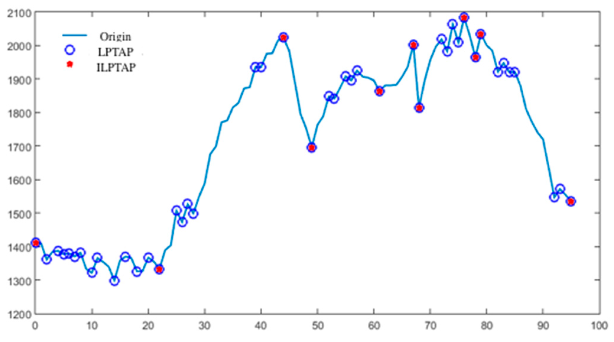
As shown in the Figure 1, taking the 96-point load curve for a substation in Nanjing, China as an example, the blue circles represent the trend alteration points detected on the curve, and a red solid point represents the ILCTAP detected on the curve.

It can be seen from the figure that the before and after trend change of the ILCTAP was clearly greater than the trend alteration points.

3.2. Weight Matrix Generation Algorithm

This algorithm first extracts the trend alteration points in the load curve as the middle curve, and then extracts the ILCTAP based on the middle curve. Different weight proportions are given to the trend alteration points and the important trend alteration points, and finally the weight matrix is obtained. The algorithm flow is as follows (Algorithm 1):

Algorithm 1. Weight Matrix Generation Algorithm.

Input: load curve$DL{C}_1=\left\{x_i\right\}$and$DL{C}_2=\left\{y_i\right\},i=1,2\dots ,n$,$epsonRate$= 0.1 Output: weight matrix$\mathrm{W}=\left\{w_i\right\},\mathrm{i}=1,2\dots ,\mathrm{n}$

Detail Algorithm Steps:

1)  Initialize weight matrix$\mathrm{W}$with all 1. 2)  According to Definition 4, extract the trends alter point to form the intermediate curve; 3)  For each load point on the middle curve, the corresponding weight increases 0.5 times; 4)  According to Definition 6, calculate the trends alter threshold ε; 5)  According to Definition 5, extract the set of important trends alter points from the intermediate curve; 6)  For each load point in the set, the corresponding weights are doubled; 7)  Return the weight matrix.

This algorithm requires only one adjusting parameter $epsonRate$. Experimental results show that the algorithm can be applied to most cases when the value of $epsonRate$ is 0.1, so $epsonRate$ defaults to 0.1. Processes of extract both the trends alter point and important trends alter point only need to scan the load curve once at most. Therefore, the time complexity of this algorithm is O(n), where n is the total number of points per day, usually 48 or 96.

3.3. Weighted Pearson Distance

In statistics, the Pearson correlation coefficient is used to reflect the linear correlation between the two variables. The corresponding concept is Pearson distance, which indicates the degree of dissimilarity between two variables. It has been widely used in the fields of text classification based on vector space model, user preference recommendation system and so on. Different from the geometric mean distance, Pearson distance emphasizes the synchronization between the two variables. Pearson distance also reflects the trend of the load curve between the similarity.

Suppose a given load curve set $DL{C}_1=\left\{x_i\right\},i=1,2,\dots ,n$ and $DL{C}_2=\left\{y_i\right\},i=1,2,\dots ,n.$ Then their Pearson coefficient and Pearson distance are:

$$\mathsf{\rho }\left(DL{C}_1,\mathrm{D}L{C}_2\right)=\frac{{{\displaystyle \sum }}_{i=1}^n\left(x_i-\overline{x}\right)\left(y_i-\overline{y}\right)}{\sqrt{{{\displaystyle \sum }}_{i=1}^n{\left(x_i-\overline{x}\right)}^2}\sqrt{{{\displaystyle \sum }}_{i=1}^n{\left(y_i-\overline{y}\right)}^2}}$$

(3)

$$\mathrm{D}\left(L_1,L_2\right)=1-\mathsf{\rho }\left(DL{C}_1,\mathrm{C}\right)$$

(4)

The weighted Pearson distance is similar to the Pearson distance and both similarly emphasize the degree of similarity of the curve’s trend. In the Pearson coefficient formula, the status of each dimension component $\left(x_i-\overline{x}\right)\left(y_i-\overline{y}\right)$ is the same, and the weight is 1. In the weighted Pearson coefficient, the contribution of each dimension is controlled by adjusting the weights of different dimensions. In the case of reasonable weight, the ability of the weighted Pearson coefficient to capture the details will be stronger than the Pearson coefficient.

Suppose given load curve sets, $DL{C}_1=\left\{x_i\right\},i=1,2,\dots ,n$ and $DL{C}_2=\left\{y_i\right\},i=1,2\dots ,n$, weight matrix $\left\{w_i\right\},i=1,2,\dots ,n$. The weighted Pearson distance calculation process is:

$$\mathrm{m}\left(DL{C}_1\right)=\frac{{{\displaystyle \sum }}_{i=1}^n{w}_i{x}_i}{{{\displaystyle \sum }}_{i=1}^n{w}_i}$$

(5)

$$\mathrm{cov}\left(DL{C}_1,\mathrm{D}L{C}_2,\mathrm{W}\right)=\frac{{{\displaystyle \sum }}_{i=1}^n{w}_i\left(x_i-m\left(DL{C}_1\right)\right)\left(y_i-m\left(DL{C}_2\right)\right)}{{{\displaystyle \sum }}_{i=1}^n{w}_i}$$

(6)

$$\mathsf{\rho }=\frac{cov\left(DL{C}_1,DL{C}_2,\mathrm{W}\right)}{\sqrt{cov\left(DL{C}_1,\mathrm{D}L{C}_1,\mathrm{W}\right)cov\left(DL{C}_2,DL{C}_2,\mathrm{W}\right)}}$$

(7)

$${\mathrm{D}}_w\left(DL{C}_1,\mathrm{D}L{C}_2\right)=1-\mathsf{\rho }\left(DL{C}_1,DL{C}_2\right)$$

(8)

This algorithm divides the contribution of common load points, trend alteration points and important trend alteration points to the Pearson’s coefficient by weight values.

If the trends of the two curves are completely similar, their trend alteration point and the important trend alteration point appear at the same position, and the weight of the corresponding time point reaches the maximum value, then the weighted Pearson coefficient degenerates to a Pearson coefficient.

If the trends of the two curves are not the same, there are some points that are trend alteration points or important trend alteration points of one curve but not of another curve. In this way, the weights on each dimension are differentiated. By enlarging the contributions of the key points to the Pearson coefficient, the Pearson coefficient is enhanced to describe the trend alterations and the clustering quality of the load curve is improved.

4. The Enhanced Pearson-Based Hierarchy Clustering Algorithm

The overall hierarchy based clustering algorithm can be described as shown in Figure 2 and the following Algorithm 2.

Algorithm 2. The Weight Pearson based Hierarchy Clustering Algorithm.

Input: A set X of Load Curves {$DL{C}_i$} Output: A cluster set$C$ /** init the C set, each load curve as a single set at the beginning**/ For i = 1 to n    $c_i=\left\{DL{C}_i\right\}$ $C=\left\{c_1,\dots ,c_n\right\}$ /** a counter for record the looping **/ $count=n+1$ /** a loop for bottom-up clustering **/  while$sizeof\left(c\right)>1$do:    /** get the minimum of the pearDist for all element **/   /** Assume: A Pearson distance function pearSimilar ($DL{C}_i,DL{C}_j$)**/   ($c_{min1}$,$c_{min2})$=minimum of pearDist ($c_i,c_j)forall{c}_i,c_{j}inC$   /** remove the minimum from current set **/   C =$C-c_{min1}-c_{min2}$   /** update the C set with new set **/   $\mathrm{C}=\mathrm{C}+\{{\mathrm{c}}_{\min 1},{\mathrm{c}}_{\min 2}\}$   index=index+1 return $\mathrm{C}$

As Figure 2 describes, the algorithm gets the load curves as input. Based on the load curves, the algorithm then creates an initial clustering set called $\mathit{C}$. As we use the bottom-up based hierarchy clustering, every load curve will become a separate set element of $\mathit{C}$. The algorithm will try to reduce the number of set elements to one. So, there begins a loop for reducing the set elements, which include three major steps. First step is to find the minimum of ${\mathit{c}}_{\mathit{i}},{\mathit{c}}_{\mathit{j}}$ in $\mathit{C}$ using the weight Pearson distance function. The weight Pearson distance function as proposed in Session Three, will return the distance between two load curves. The second step is to remove ${\mathit{c}}_{\mathit{i}},{\mathit{c}}_{\mathit{j}}$ from $\mathit{C}$. And the final step is to add new element $\{{\mathbf{c}}_{\mathbf{min}1},{\mathbf{c}}_{\mathbf{min}\mathbf{2}}\}$ into the $\mathit{C}$. As the loop goes, the size of $\mathit{C}$ will reduce, and finally form the result set. The detailed algorithm pseudo-code is shown as Algorithm 2. The time complexity of our algorithm is about ${\mathit{n}}^{\mathbf{2}}\mathbf{log}\mathbf{\left(}\mathit{n}\mathbf{\right)}$, which is like the traditional hierarchy clustering.

5. Experiment and Results Analysis

5.1. Experimental Data

The experiments in this paper are based on two daily load data sets,

Table 2. Experimental dataset table.

	Daily Load Points	Training Data	Test Data
Data set 1	48	730 days	31 days
Data set 2	96	274 days	15 days

shows the details.

Data set 1: The daily load data of a European substation provided by the East-Slovakia Power Distribution Company. The load data comes from a research paper [22].

Data set 2: The daily load data of a substation in Nanjing, China (the dataset can be obtained on request from email address [email protected], the unit of the Nanjing data is MW)

5.2. Experimental Method

As the hierarchy clustering consumes more time than K-Means, we apply the K-Means algorithm for an initial clustering. After the initial clustering, the original dataset is divided into k sub-datasets. For each sub-dataset, the weighted Pearson hierarchy clustering algorithm is applied for further clustering. Detail procedure is as Figure 3.

After the hierarchy clustering, the final clusters are formed. In order to evaluate the clustering accuracy, we use a SVM model for the evaluation. The clustering results are used as the training label of SVM model. So the quality of the SVM prediction will rely on the clustering quality.

To measure the results, some indicators are introduced, which include mean absolute percentage error and maximum absolute error.

Mean absolute percentage error:

$$\mathrm{MAPE}=100\times \frac{1}{n}{\displaystyle \sum }_{i=1}^n\left|\frac{L_{R_i}-L_{P_i}}{L_{R_i}}\right|$$

(9)

Maximum absolute error:

$$\mathrm{M}=\max \left(\left|L_{R_i}-L_{P_i}\right|\right)$$

(10)

For the above formula, n is the number of test samples, i is the index of the test samples, $L_{R_i}$ is the highest load real value of the ith test sample and $L_{P_i}$ is the corresponding highest load forecast.

5.3. Analysis of the Experimental Results

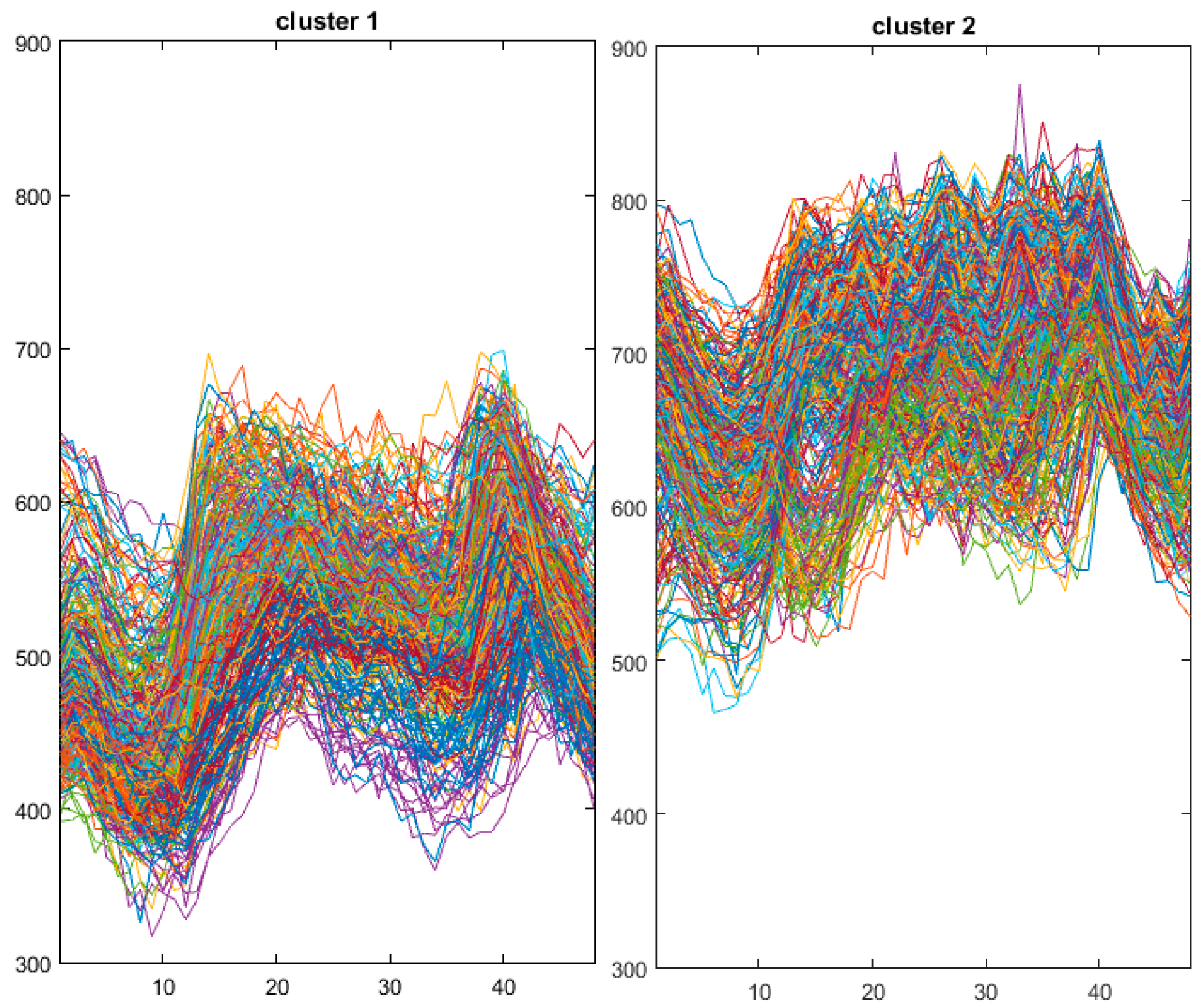
For this part, the 730 daily load curve in data set 1 are clustered. The clustering results of the first time are shown in Figure 4, the whole data set is divided into two clusters. Cluster 1 expresses the low level load samples of overall samples. Cluster 2 expresses the high level load samples of overall samples.

The typical profiles of these two clusters are shown Figure 5, high load samples are maintained at a higher load levels from 7 a.m. to 10 p.m. and reached a peak between 7 p.m. and 8 p.m. Low load samples are also at a period of intensive use from 7 a.m. to 10 p.m. however, they reach a trough between 3 p.m. and 7 p.m. The separate statistics of daily average temperature of the two classes of samples indicate that the average temperature of high level load samples is 15.77 °C (60.3 F) and the average temperature of low level load samples is 1.62 °C (34.9 F). It is obvious that these two kinds of electricity behavior are closely related to the temperature.

Figure 6 shows separate statistics of the distribution of the two classes’ dates among the 12 months of a year. It is obvious that the dates of low level load samples are mainly distributed from April to October (the blue part in the middle) and the highest temperature during this time is only 26.5 °C (79.7 F), the climate is cool. The dates of high level load samples are mainly distributed from November to April of the following year (the red part of two sides) and the lowest temperature during this time is −14.2 °C (6.44 F), the climate is cold. From the above, the electricity behavior of high load samples is speculated to mainly be caused by the heating power due to the low temperature. This part of power leads to the higher load level of the whole day. The electricity behavior of low load samples is mainly influenced by daily work habits and life. Because of the high latitudes, the temperature is appropriate in summer and autumn so the demand for refrigeration is weak. Thus, the whole day load levels of summer and autumn are lower than spring and winter.

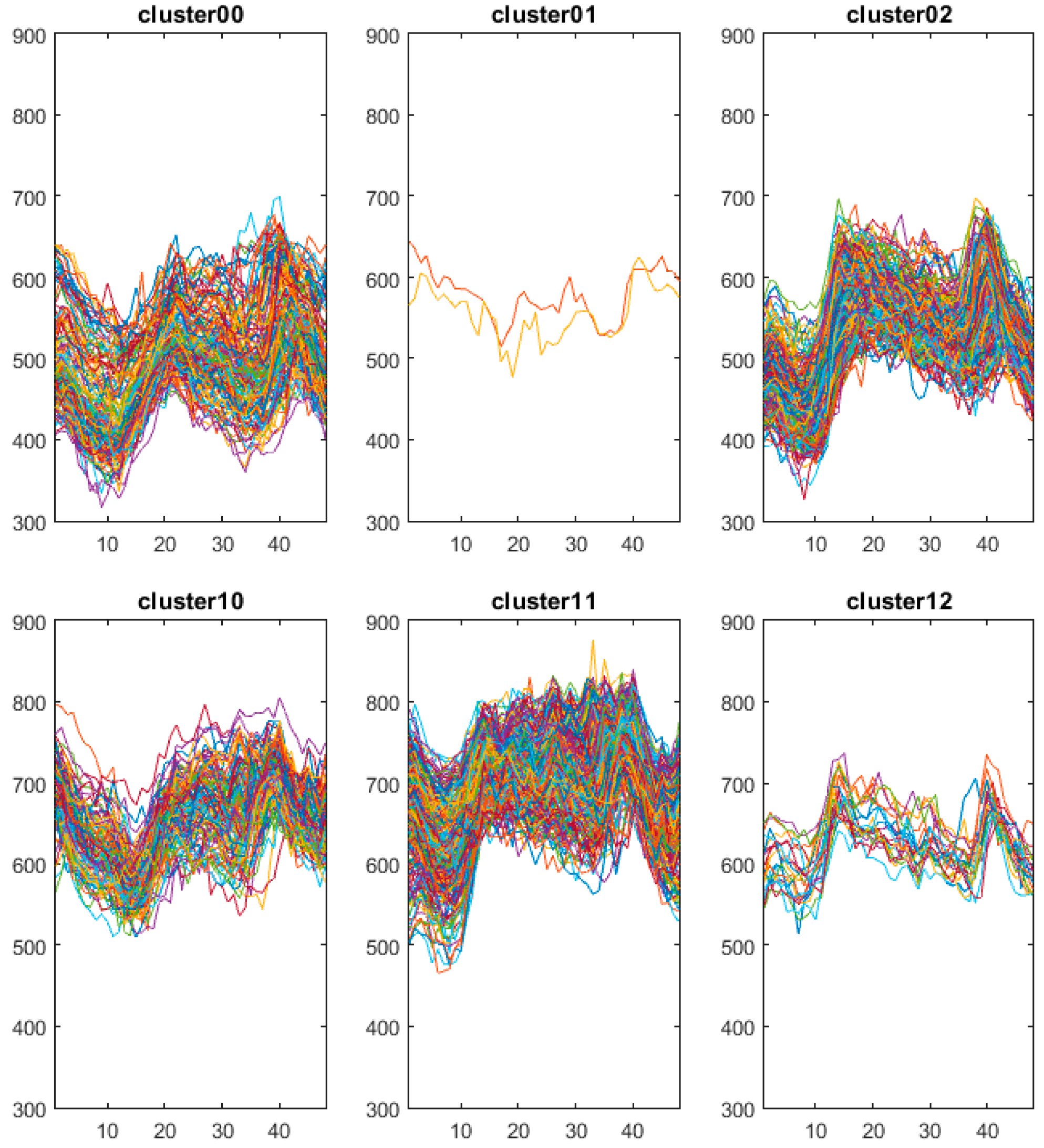
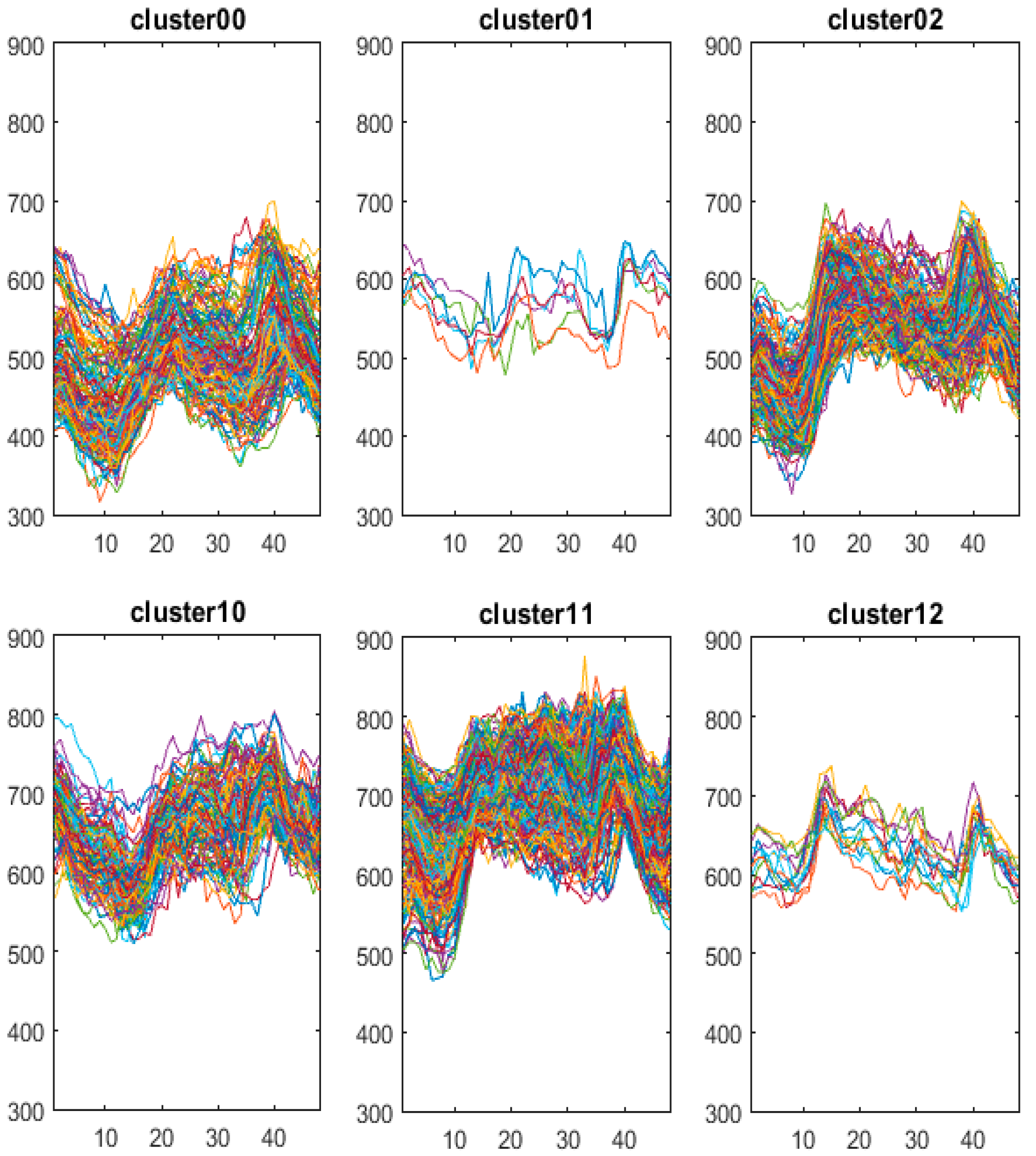
Pearson distance and weighted Pearson distance are used for comparing the similarity measurements in the second clustering. According to this method, the above two clusters are subdivided into three clusters. Figure 7 shows the Pearson distance clustering result and Figure 8 shows the weighted Pearson distance clustering result.

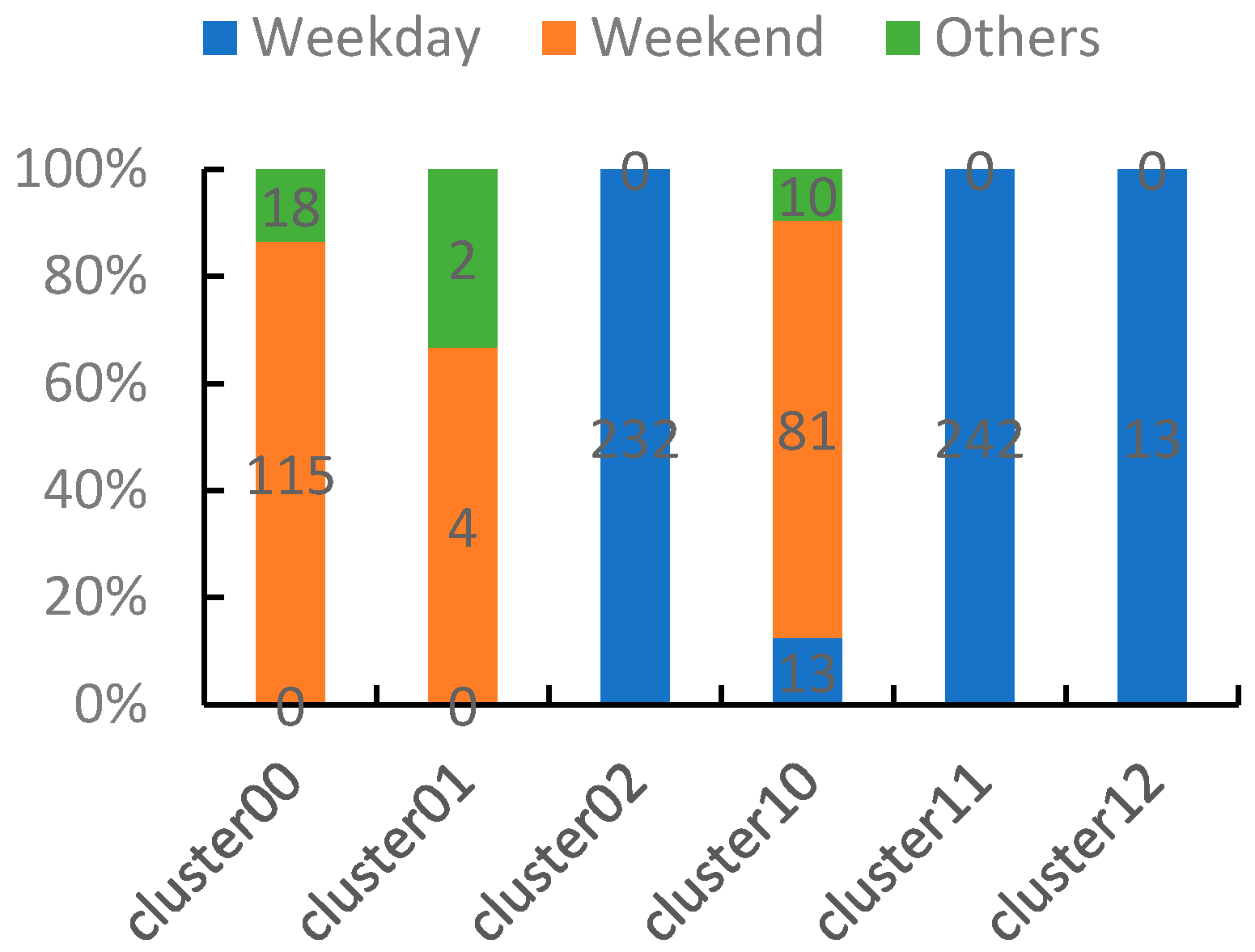
From the statistics of the two experiments, Figure 9 and Figure 10 show the corresponding date of the type distribution about the load samples of the six clusters.

Overall, the structures of these two distributions are very similar: For low level load samples, the workday load curves are mainly in cluster 02 and non-workday load curves are mainly in cluster 00 and cluster 01. For high level load samples, the workday load curves are mainly in cluster 11 and cluster 12 and non-workday load curves are mainly in cluster 10.

However, there are slight differences between the corresponding clusters of the two distributions. Take cluster 01 for example, this cluster only has two daily load samples 89, 90 corresponding to 30 March 1997 and 31 March 1997 (are all legal holidays) in the Pearson distance experiment, while in the weighted Pearson distance experiments, there are four more daily load samples, they are 6 April 1997, 12 April 1997, 13 April 1997 and 27 April 1997 (these days are all weekends). From the aspect of the date, these four days are all the weekends of April which are very closed to Easter. From the aspect of the real life, the electricity behavior of these dates are very likely to be affected by the celebrations of various industries during Easter. Therefore, it is fair and reasonable to put them into cluster 01.

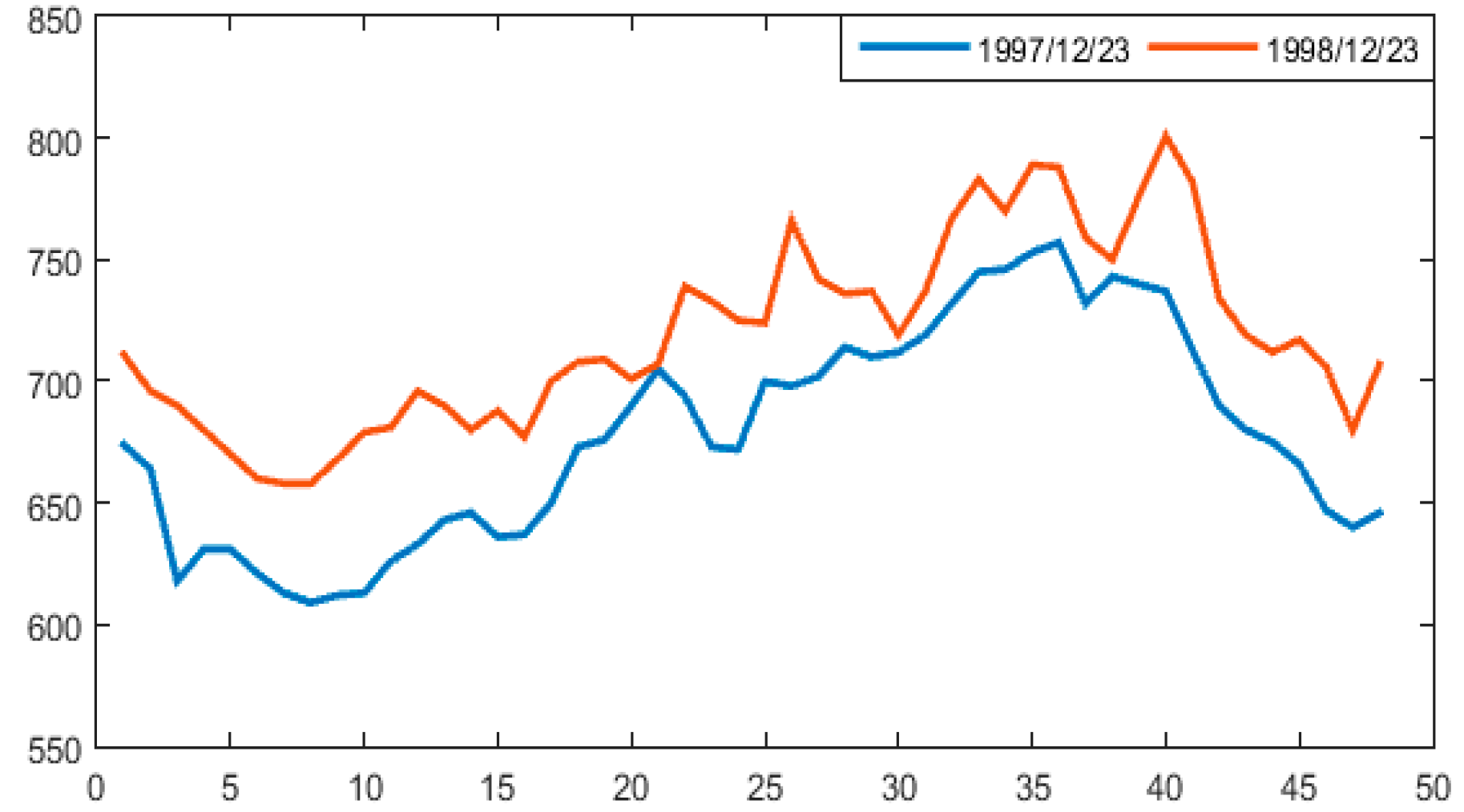
According to the comparison of cluster 10 and cluster 11, for the Pearson distance experiment, the dates 23 December 1997 and 23 December 1998 are put into the cluster 11 which is the same as the workday load curve of winter and spring. However, in the weighted Pearson distance experiments, these two days are put into the cluster 10 which is the same as the non-workday load curve of winter and spring. Considering that 23 December is close to Christmas Eve and Christmas Day, it is much more reasonable that the rule of the power consumption should be close to that of holidays. Figure 11 shows the typical profiles of the three clusters of high load samples. Comparing Figure 11 with Figure 12, it is obvious that the electricity behaviors of 23 December 1997 and 23 December 1998 are much more similar to cluster10 (blue curve) than cluster11 (orange curve).

A SVM prediction model is constructed for predicting the daily maximum load value from 1 January 1999 to 31 January 1999. Before the prediction, the test samples should be matched to the above clusters. The matching results of these two experiments are identical: 12 days are matched to cluster 10 and 19 days are matched to cluster 11. According to the members in cluster 10 and cluster 11 used to construct the SVM predictors separately, the predicted results are shown in the figures below (Figure 13 and Figure 14). Predict 1 refers to the predicted value of the Pearson experiment and Predict 2 refers to the predicted value of the weighted Pearson experiment. In mid- to late of January, the two prediction curves almost overlap. In early January, the value of Predict 2 is closer to the real value than Predict 1.

Then, we run the same kind of multiple clustering algorithm and SVM prediction algorithm on dataset 2. The predicted results are shown in the figures below. Predict 1 refers to the prediction value of the Pearson experiment and Predict 2 refers to the prediction value of the weighted Pearson experiment. In the predictive results of upper left, Predict 1 and Predict 2 almost overlap. In the lower right predictive results, the value of Predict 2 is much closer to the real value than Predict 1 for most cases.

Table 3. The calculation results of short-term load prediction evaluation index.

Dataset	Similarity Measurement	MAPE Indexes	M Indexes
Dataset 1	Pearson distance	1.7782	32.9898
	Weighted Pearson distance	1.7638	31.7687
The percentage of optimization		+0.81%	+3.70%
Dataset 2	Pearson distance	3.7721	219.3205
	Weighted Pearson distance	3.1711	158.6972
The percentage of optimization		+15.93%	+27.64%

shows the prediction evaluation index of all the above experiments separately. According to Table 3, for both dataset 1 and dataset 2, the load forecasting results of the weighted Pearson distance as the second clustering similarity measurement are better than the Pearson distance ones. The percentage of optimization is defined as P-W/W (where P is Pearson distance; W is weighted Pearson distance). It is obvious that the optimization effect of dataset 2 is better than dataset 1. This is due to the capacity of capturing the dramatic profile trend alteration points of the weighted Pearson distance method is much stronger. There are two main reasons for those points with dramatic changes on the load curve:

• The collecting location of dataset 2 is Nanjing (China). and the collecting location of dataset 1 is northern Europe. As a result of the differences of some factors like weather and population, the daily load power changes for northern Europe are pretty stable. However, the change of daily load power for Nanjing is a little more severe. For example, the summer climate in northern Europe is cool and the maximum temperature is just 26.5 °C, but the summer climate in Nanjing is torrid, so the demand of refrigeration is sometimes much higher. There also exists randomness in residents’ daily activities and use of power. All the above reasons explain the change of daily load power in Nanjing being more frequent and severe.
• The scope of transformer substation for dataset 1 should be larger than for dataset 2. More users means that the influence of arbitrariness for individual electricity behavior on the overall load curve will be weakened. Thus, the load curve of dataset 1 is pretty stable, the weight numbers of each dimension for the weighted Pearson distance are very similar so that the effect of optimization is not clear.

The clustering effect of the weighted Pearson distance experiments is much better than the Pearson distance experiments. Especially for some special curves, such as the dates before and after major holidays, the division results of the weighted Pearson distance experiments are more reasonable. In the application of short-term load prediction, the weighted Pearson distance has a function of tiny adjustment to the members of each cluster so that the samples used for constructing the SVM predictor are much more similar. Thus, the prediction results of the weighted Pearson distance experiments are more accurate than those of the Pearson distance experiments.

6. Conclusions

In this paper, we proposed a weight matrix generation algorithm based on load trend alteration points, and combine the weighted Pearson distance to form a new weighted Pearson-based hierarchy clustering algorithm. The comparison between the daily load datasets of a substation in Europe and the daily load dataset of a substation in Nanjing (China) shows that the weighted Pearson distance has more sensitive load trend characterization ability than the Pearson distance. The cluster trend curves of the load curves are more similar and more in line with the facts. At the same time, clustering results of the weighted Pearson distance are applied to the short-term load forecasting based on two different datasets, and the prediction quality is improved to some extent, which proves that the clustering algorithm has certain universality. Therefore, the multi-clustering method based on Euclidean distance and the weighted Pearson distance proposed in this paper is of great value in practical engineering calculations. In future, we will try to apply the weighted Pearson distance to other clustering algorithms to improve the performance of those algorithms.

References

- Chicco, G. Overview and performance assessment of the clustering methods for electrical load pattern grouping. Energy 2012, 42, 68–80. [Google Scholar] [CrossRef]
- McLoughlin, F.; Duffy, A.; Conlon, M. Evaluation of time series techniques to characterise domestic electricity demand. Energy 2013, 50, 120–130. [Google Scholar] [CrossRef] [Green Version]
- Azad, S.A.; Ali, A.B.M.S.; Wolfs, P. Identification of typical load curve using K-Means clustering algorithm. In Proceedings of the Asia-Pacific World Congress on Computer Science and Engineering, Nadi, Fiji, 4–5 November 2014. [Google Scholar]
- Nafkha, R.; Gajowniczek, K.; Ząbkowski, T. Do Customers Choose Proper Tariff? Empirical Analysis Based on Polish Data Using Unsupervised Techniques. Energies 2018, 11, 514. [Google Scholar] [CrossRef]
- Pérez-Chacón, R.; Luna-Romera, J.M.; Troncoso, A.; Martínez-Álvarez, F.; Riquelme, J.C. Big Data Analytics for Discovering Electricity Consumption Patterns in Smart Cities. Energies 2018, 11, 683. [Google Scholar] [CrossRef]
- Kesemen, O.; Tezel, Ö.; Özkul, E. Fuzzy c-means clustering algorithm for directional data (FCM4DD). Expert Sys. Appl. 2016, 58, 76–82. [Google Scholar] [CrossRef]
- Rhodes, J.D.; Cole, W.J.; Upshaw, C.R.; Edgar, T.F.; Webber, M.E. Clustering analysis of residential electricity demand profiles. Appl. Energy 2014, 135, 461–471. [Google Scholar] [CrossRef]
- McLoughlin, F.; Duffy, A.; Conlon, M. A clustering approach to domestic electricity load curve characterisation using smart metering data. Appl. Energy 2015, 141, 190–199. [Google Scholar] [CrossRef]
- Räsänen, T.; Voukantsis, D.; Niska, H.; Karatzas, K.; Kolehmainen, M. Data-based method for creating electricity use load curve using large amount of customer-specific hourly measured electricity use data. Appl. Energy 2010, 87, 3538–3545. [Google Scholar] [CrossRef]
- Hernández, L.; Baladrón, C.; Aguiar, J.M.; Carro, B.; Sánchez-Esguevillas, A. Classification and clustering of electricity demand patterns in industrial parks. Energies 2012, 5, 5215–5228. [Google Scholar]
- Vercamer, D.; Steurtewagen, B.; Van den Poel, D. Predicting consumer load curve using commercial and open data. IEEE Trans. Power Syst. 2016, 31, 3693–3701. [Google Scholar] [CrossRef]
- Pereira, R.; Fagundes, A.; Melício, R.; Mendes, V.M.F.; Figueiredo, J.; Martins, J.; Quadrado, J.C. A fuzzy clustering approach to a demand response model. Int. J. Electr. Power Energy Syst. 2016, 81, 184–192. [Google Scholar] [CrossRef] [Green Version]
- Abdulaal, A.; Asfour, S. A Fuzzy Genetic Algorithm classifier: The impact of time-series load data temporal dimension on classification performance. In Proceedings of the 2016 15th IEEE International Conference on Machine Learning and Applications (ICMLA), Anaheim, CA, USA, 18–20 December 2016. [Google Scholar]
- Varga, E.D.; Beretka, S.F.; Noce, C.; Sapienza, G. Robust real-time load curve encoding and classification framework for efficient power systems operation. IEEE Trans. Power Syst. 2015, 30, 1897–1904. [Google Scholar] [CrossRef]
- Harvey, P.R.; Stephen, B.; Galloway, S. Classification of AMI residential load profiles in the presence of missing data. IEEE Trans. Smart Grid 2016, 7, 1944–1945. [Google Scholar] [CrossRef]
- Zhong, J.X.; Wang, J.; Yu, X.H.; Wang, Q.M.; Combariza, M.; Holmes, G. Hybrid Load Profile Clustering for identifying patterns of electricity consumers. In Proceedings of the 2016 IEEE 25th International Symposium on Industrial Electronics (ISIE), Santa Clara, CA, USA, 8–10 June 2016. [Google Scholar]
- Singh, S.; Yassine, A. Big data mining of energy time series for behavioral analytics and energy consumption forecasting. Energies 2018, 11, 452. [Google Scholar] [CrossRef]
- Jia, H.M.; He, G.Y.; Fang, C.X.; Li, K.W.; Yao, Y.Z.; Huang, M.M. Load forecasting by multi-hierarchy clustering combining hierarchy clustering with approaching algorithm in two directions. Power Syst. Technol. 2007, 31, 33–36. [Google Scholar]
- Teeraratkul, T.; O’Neill, D.; Lall, S. Shape-based approach to household electric load curve clustering and prediction. IEEE Trans. Smart Grid 2018, 9, 5196–5206. [Google Scholar] [CrossRef]
- Basu, K.; Debusschere, V.; Douzal-Chouakria, A.; Bacha, S. Time series distance-based methods for non-intrusive load monitoring in residential buildings. Energy Build. 2015, 96, 109–117. [Google Scholar] [CrossRef]
- Al-Wakeel, A.; Wu, J.Z.; Jenkins, N. K-Means based load estimation of domestic smart meter measurements. Appl. Energy 2017, 194, 333–342. [Google Scholar] [CrossRef]
- Abbas, S.R.; Arif, M. Electric load forecasting using support vector machines optimized by genetic algorithm. In Proceedings of the 2006 IEEE Multitopic Conference, Islamabad, Pakistan, 23–24 December 2006. [Google Scholar]
Figure 1.
Daily LCTAP and ILCTAP.
Figure 2.
The overall flowchart of the weighted Pearson-based hierarchy clustering algorithm.
Figure 3.
The experimental procedure.
Figure 4.
Clustering results (the left sub-figure includes low level load samples, the right sub-figure includes high level load samples).
Figure 5.
Typical load curve from Figure 4 (blue for cluster 1, and red for cluster 2).
Figure 6.
Month distribution of cluster 1 and cluster 2 (axis x for the months and axis y for the numbers of users).
Figure 7.
Original Pearson results.
Figure 8.
Weighted Pearson results.
Figure 9.
Weekday distribution of the original Pearson results.
Figure 10.
Weekdays distribution of Weighted Pearson Results.
Figure 11.
Typical load curves of clusters 10, 11, 12.
Figure 12.
Two typical days’ load curves.
Figure 13.
Load curve comparison (Predict 2 is our method).
Figure 14.
Deviation analysis of real, original Pearson and weighted Pearson.