Article

Applications of a Strong Track Filter and LDA for On-Line Identification of a Switched Reluctance Machine Stator Inter-Turn Shorted-Circuit Fault

1
College of Information Engineering, Tianjin University of Commerce, Tianjin 300134, China
2
College of Control Science and Engineering, Hebei University of Technology, Tianjin 300130, China
3
College of Electrical Engineering, Zhejiang University, Hangzhou 310027, China
*
Author to whom correspondence should be addressed.
Energies 2019, 12(1), 134; https://doi.org/10.3390/en12010134
Submission received: 4 September 2018 / Accepted: 19 September 2018 / Published: 1 January 2019
(This article belongs to the Special Issue Optimization Methods Applied to Power Systems)

Abstract

:
Reliability is pivotal significance for switched reluctance machine drives (SRD) applied to safety essential transportation and industrial fields. An inter-turn shorted-circuit fault (ISCF) could incite the machine to operate in unbalanced status, resulting in the noise increases. In the event such a fault remains untreated, the fault will further destroy the rest of the normal phases, even leading to a tragic incident for the entire drive application. To improve the reliability of SRD, an efficient on-line fault diagnosis method for ISCF should be proposed. This paper is focused on employing the strong track filter (STF) to achieve real-time phase resistance differences between before and after ISCF, which are used as features to diagnose the fault occurrence and the fault phase. Furthermore, a classification namely as linear discriminant analysis (LDA) is selected to estimate fault severity. Finally, simulation and experiments correspond to various running statuses are executed and their results can verify that the diagnosis method has accuracy and robustness.

1. Introduction

In the past decade, switched reluctance machines and their drives have obtained a great deal of regards and have been applied to transportation and industrial applications, including aerospace, power traction, hybrid vehicles [1]. Switched reluctance machines’ (SRM) structure is simple, without any permanent magnets and windings on the rotors [2]. It is very favorable for machine running in the rigorous circumstance owing to its remarkable fault tolerance, superior efficiency and wonderful reliability. The switched reluctance machine drives (SRD) has the capability of fault tolerance naturally, but is not absolutely fault free [3]. In the case where the SRM operates perennially, faults will possibly occur in the motor and its power convert. For SRM, the inter-turn shorted-circuit fault (ISCF) generally leads to unbalanced magnetic pull, high torque ripples, over-current, and lower load ability, yet would not influence the operation of the rest normal phases in the case where a small number of windings failed, due to the independence of excitation and control mode between windings of each phase. Thus, the ISCF is often overlooked, which results in a higher temperature and further damage the insulation system of the motor. Regarding this issue, it is essential to elevate the SRM with a certain ability to diagnose the ISCF. Thus, the progressive diagnosis method plays an important role for heightening safe operation and reliability for SRMs, which is the main issue of this paper.
In regard to detecting the ISCF, many methods have been reported. All the methods could be classified into two types: feature extraction and intelligent recognition. For the feature extraction method, the distinctive between normal and fault machine performance can be presented by the amplitudes or frequencies of extracted signatures, which is used to realize the fault detection. As well as the common fault features include current, voltage, and vibration. In [4], the forward and backward rotating currents were measured, and their negative sequence components were extracted to detect inter-turn faults powerfully for induction motors. For permanent magnet synchronous motor, a combination of the values of the voltages and the stator currents obtain by wavelet transform was considered as the fault feature to diagnose the inter-turn faults in the literature [5]. In [6], the external vibration coupled with the stray magnetic field was analyzed to receive the vibration spectrum distinctions of healthy and faulty motor to implement non-invasive diagnosis for the rotor windings fault of the synchronous machine. Additionally, a number of intelligent recognition diagnosis methods have been used for the ISCF identification, such as neural networks, genetic algorithm, and support vector machines [7,8,9].
Comparing to other types of motors, the ISCF for SRMs has been investigated insufficiently. The fault mechanism was introduced in [1,2,3,10]. Recently, a modeling method for the ISCF with one shorted coil in SRM was presented in [11]. Fault diagnosis methods were investigated in [12,13,14]. A diagnosis technology based on tracking the maximum current point was presented to detect the fault occurrence and faulty degree by [12]. However, the diagnosis method is just applied to the fault occurring in only one phase winding. In [13], the fundamental components were extracted to reconstruct based on spectrum analysis, and components of reconstructed current were treated as the features to detect fault. In [14], an extended Kalman filter (EKF) was used to achieve a precise response in initial moments after inter-turn winding failure. In fact, the diagnosis method proposed in literature [13,14] could only detected the fault occurrence, but the detection of faulty phase and severity have not been implemented.
Indeed, the EKF can quickly confirm the fault appearance, so it has been already related to applications in fields of fault monitoring and diagnosing [15,16]. However, the EKF is similar to the open-loop system, which leads to the tracking results are not desired even divergent in certain case, such as in the mutation state [17]. Comparing to the tracking performance of EKF, the strong track filter (STF) is more robust for the uncertain faulty model, better tracking especially in the mutation state, and less complex for calculation. Hence, the STF algorithm is substituted for the EKF algorithm to use in the fault diagnose scheme in this paper.
Additionally, the developing of diagnosis mode always lack enough samples since the fault samples are obtained difficultly in industrial processes. This may cause the overfitting problem in case the model is developed by nonlinear methods [18]. However, linear discriminant analysis (LDA) has the capability of dimensionality reduction and supervised classification. Using LDA based on grabbling for the vintage discriminant direction of the samples, the data between different classes can be separated maximumly and robustly. Thus, LDA has been successfully utilized in detecting and monitoring for industrial applications [19,20]. In [21], it is suggested that LDA is not only used to diagnose fault type but also suitable to estimate the faulty severity. In this paper, LDA is especially adopted to estimate the fault severity.
The rest of the paper is arranged as follows: In Section 2, a faulty SRM model and the failure mechanism are elaborated. In Section 3, the STF procedure utilized in the faulty SRM is analyzed. In Section 4, the ISCF detection schemes, including the fault occurrence, faulty phases are explained in detail. Additionally, the major conception of LDA and how it is employed for the fault severity identification are also described in this section. Finally, to demonstrate effectiveness and evaluate the robustness of the diagnostic method, simulation results as well as online experimental results corresponding to different scenarios are all presented in Section 5.

2. Model of Switched Reluctance Machine (SRM) and the Failure Mechanism Analysis

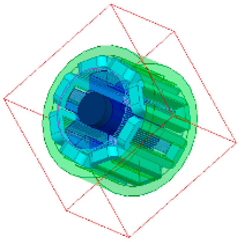
2.1. Model of the Healthy SRM

The structure of the SRM utilized in this paper is described in Figure 1 which is a four-phase 8/6 motor. For SRMs, when the coil of a phase is excited, the magnetic flux always closes along the path with the minimized magnetic reluctance. The electromagnetic torque is produced by the energy conversion in a coil.
Each phase voltage involved two parts: the resistive voltage drop and the derivative of the flux linkage, that can be given by:
U n = R n i n + d ψ n d t
where Un is the phase voltage, in is the phase current, and ψn and Rn are, separately, the flux linkage and the resistance for each phase. Parameter n expresses the number of phase (n = A, B, C, D).
The flux linkage is expressed in Equation (2):
ψ n = L n ( i n , θ ) i n
where Ln (in, θ) is the inductance per phase. Because the term Ln (in, θ) contains parameters in and θ. Equation (1) can be replaced with:
U n = R n i n + d θ d t d L n ( i n , θ ) d θ i n + L n ( i n , θ ) d i n d t
The rotational velocity ω is shown in the following equation:
ω = d θ d t
Hence, both sides of the Equation (3) are simultaneously multiplied by the phase current in, the power balance is found by:
U n i n = R n i n 2 + d L n ( i n , θ ) d θ i n 2 ω + i n L n ( i n , θ ) d i n d t
When the winding is energized, if the losses of the phase winding can be ignored, a part of the input power is used to make the energy storage in the winding increased, and the other part is converted to output mechanical power. Hence, the electromagnetic torque per phase is found by:
T n = 1 2 i n 2 d L n ( i n , θ ) d θ
The Newton motion law for the SRM is given by:
J d ω d t = n = 1 4 T n T L F ω
where J, F, TL are respectively moment inertia, damping coefficient and the load torque. Therefore, Equation (7) can be replaced with:
J d ω d t + F ω = 1 2 n = 1 4 i n 2 d L n ( i n , θ ) d θ T L

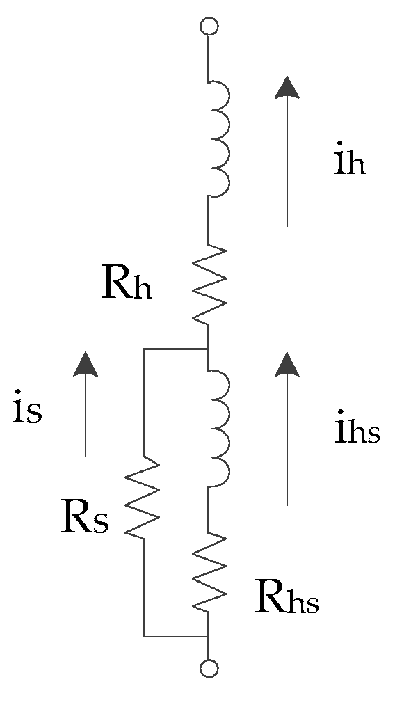
2.2. The Failure Mechanism Analysis

The equivalent circuit of the faulty coil is illustrated in Figure 2. ISCF could be cause by the insulation of windings. Due to the ISCF, a route with a certain resistance should be produced between the two turns.
The voltage equation of the fault phase is found by:
U n = i h R n + i s R s + ( N h N s ) d ψ s d t + N h n 4 d ψ n d t
where Un is the supplied voltage of the fault phase. Parameters Rn is the resistance in healthy turns, parameters Rhs is the resistance in shorted turns, as well as Rs is the resistance of the short-circuit route, which amplitude is very small. Parameters Nh is the number of healthy turns, and Ns is the short-circuit turn number. ψn is the magnetic flux of a healthy pole, ψs is the magnetic flux of a short-circuit pole. Parameters ih, ihs and is are currents, respectively flowing in healthy turns of the faulty pole, the shorted turns, and the short-circuit route. The relationship between three parameters is as follows:
i h = i h s + i s
Moreover, the voltage drop of the resistance of the short-circuit route, Rsis is denoted by:
R s i s = R h s i h s + N s d ψ s d t
Therefore, the current flowing in shorted turns can be obtained from Equations (10) and (11):
i h s = R s i h R s + R h s N s ( d ψ s / d t ) R s + R h s
The current flowing in the shorted turns could be represented by:
i p = N s ( d ψ s / d t ) r ( R s r + N s )
where r is assumed as the resistance of each turn.

3. The STF Procedure

The state equation of the SRD is described as follows:
x ( k + 1 ) = A ( k , x ( k ) ) x ( k ) + u ( k )
where the vector x(k) as a variable, is estimated by STF, and defined as:
x ( k ) = [ i 1 ( k ) i 2 ( k )   i 3 ( k )   i 4 ( k )   θ ( k )   ω ( k )   R ( k )   T L ] T
Thus, the model of the SRM in the discrete-time state-space is described by the Equations (16)–(23), which include four currents, angular position, rotor angular position, phase resistance and load torque.
f 1 = i 1 ( k + 1 ) = i 1 ( k ) + [ u 1 ( k ) R 1 ( k ) i 1 ( k ) d L 1 ( i 1 , θ ) d θ i 1 ( k ) ω ( k ) ] t s L 1 [ θ ( k ) ]
f 2 = i 2 ( k + 1 ) = i 2 ( k ) + [ u 2 ( k ) R 2 ( k ) i 2 ( k ) d L 2 ( i 2 , θ ) d θ i 2 ( k ) ω ( k ) ] t s L 2 [ θ ( k ) ]
f 3 = i 3 ( k + 1 ) = i 3 ( k ) + [ u 3 ( k ) R 3 ( k ) i 3 ( k ) d L 3 ( i 3 , θ ) d θ i 3 ( k ) ω ( k ) ] t s L 3 [ θ ( k ) ]
f 4 = i 4 ( k + 1 ) = i 4 ( k ) + [ u 4 ( k ) R 4 ( k ) i 4 ( k ) d L 4 ( i 4 , θ ) d θ i 4 ( k ) ω ( k ) ] t s L 4 [ θ ( k ) ]
f 5 = θ ( k + 1 ) = θ ( k ) + ω ( k ) t s
f 6 = ω ( k + 1 ) = ω ( k ) + 1 J [ 1 2 n = 1 4 i n 2 ( k ) d L n ( i n , θ ) d θ T L F ω ( k ) ] t s
f 7 = R 1 ( k + 1 ) = R 1 ( k )
f 8 = T L ( k + 1 ) = T L ( k )
In order to govern the relationship among above state vectors, the transition matrix A is required which is defined as:
A ( k , x ( k ) ) = [ a 11 0 0 0 0 a 16 a 17 0 0 a 22 0 0 0 a 26 0 0 0 0 a 33 0 0 a 36 0 0 0 0 0 a 44 0 a 46 0 0 0 0 0 0 a 55 a 56 0 0 a 61 a 62 a 63 a 64 0 a 66 0 a 68 0 0 0 0 0 0 a 77 0 0 0 0 0 0 0 0 a 88 ]
Additionally, each element in transition matrix A are acquired as:
a 11 = f 1 i 1 = 1 [ R 1 ( k ) + d L 1 ( θ ( k ) ) d θ ω ( k ) ] t s L 1 ( θ ( k ) )
a 16 = f 1 ω = d L 1 ( θ ( k ) ) d θ i 1 ( k ) L 1 ( θ ( k ) ) t s
a 17 = f 1 R 1 = i 1 ( k ) L 1 ( θ ( k ) ) t s
a 22 = f 2 i 2 = 1 [ R 2 ( k ) + d L 2 ( θ ( k ) ) d θ ω ( k ) ] t s L 2 ( θ ( k ) )
a 26 = f 2 ω = d L 2 ( θ ( k ) ) d θ i 2 ( k ) L 2 ( θ ( k ) ) t s
a 33 = f 3 i 3 = 1 [ R 3 ( k ) + d L 3 ( θ ( k ) ) d θ ω ( k ) ] t s L 3 ( θ ( k ) )
a 36 = f 3 ω = d L 3 ( θ ( k ) ) d θ i 3 ( k ) L 3 ( θ ( k ) ) t s
a 44 = f 4 i 4 = 1 [ R 4 ( k ) + d L 4 ( θ ( k ) ) d θ ω ( k ) ] t s L 4 ( θ ( k ) )
a 46 = f 4 ω = d L 4 ( θ ( k ) ) d θ i 4 ( k ) L 4 ( θ ( k ) ) t s
a 55 = f 5 θ = 1
a 56 = f 5 ω = t s
a 62 = f 6 i 2 = 1 J i 2 ( k ) d L 2 ( θ ( k ) ) d θ t s
a 63 = f 6 i 3 = 1 J i 3 ( k ) d L 3 ( θ ( k ) ) d θ t s
a 64 = f 6 i 4 = 1 J i 4 ( k ) d L 4 ( θ ( k ) ) d θ t s
a 66 = f 6 ω = 1 F J t s
a 68 = f 6 T L = 1 J t s
a 77 = f 7 R 1 = 1
a 88 = f 8 T L = 1
Since the transition matrix A(k, x(k)) contains the variable state vector x(k), the STF is employed to obtain the estimated resistance based on easily measured outputs in order to eliminate negative impacts caused by load disturbance or inaccurate model. The STF is organized as follows.
The measurement equation is shown as:
{ x ( k + 1 ) = f ( k , x ( k ) , u ( k ) ) + σ ( k ) y ( k + 1 ) = h ( k + 1 , x ( k + 1 ) , u ( k + 1 ) ) + ϖ ( k )
where f( ) is the state transition function and h( ) is the nonlinear transformation function. u(k) is the control variable, σ(k) is the process noise. Q(k) is symmetric and positive definite matrix. R(k) is a covariance matrix, which is symmetric positive definite. ϖ(k) is the matrix of the measurement noise, which are all irrelevant to initial value of state variable x(0).
The estimated value with one procedure of the state variable is given as:
x ^ ( k + 1 | k ) = f ( k , x ^ ( k | k ) , u ( k ) )
The residual matrix and the gain matrix are respectively defined as Equations (45) and (46):
ϒ ( k + 1 ) = y ( k + 1 ) y ^ ( k + 1 ) = y ( k + 1 ) h ( k + 1 , x ^ ( k + 1 | k ) )
K ( k + 1 ) = P ( k + 1 | k ) H T ( k + 1 , x ^ ( k + 1 | k ) ) ( H ( k + 1 , x ^ ( k + 1 | k ) ) P ( k + 1 | k ) H T ( k + 1 , x ^ ( k + 1 | k ) ) + R ( k ) ) 1
Calculating the predicted error covariance matrix:
P ( k + 1 | k ) = λ ( k + 1 ) F ( k , x ^ ( k | k ) , u ( k ) ) P ( k | k ) F T ( k , x ^ ( k | k ) , u ( k ) ) + Q ( k )
The state estimated error covariance matrix is calculated by:
P ( k + 1 | k ) = [ I K ( k + 1 ) H ( k + 1 , x ^ ( k + 1 | k ) ) ] P ( k + 1 | k )
The steps of calculating the fading factor can be summarized as Equations (49)–(53):
λ ( k + 1 ) = { c i λ 0   , c i λ 0 1   1 , c i λ 0 < 1
where ci is the predetermined constant, and λ0 can be obtained by Equations (50)–(52):
λ 0 = t r [ N ( k + 1 ) ] t r [ M ( k + 1 ) ]
N ( k + 1 ) = V ( k + 1 ) H ( k + 1 , x ^ ( k + 1 | k ) ) Q ( k ) H T ( k + 1 , x ^ ( k + 1 | k ) ) β R ( k )
M ( k + 1 ) = H ( k + 1 , x ^ ( k + 1 | k ) ) F ( k , x ^ ( k | k ) , u ( k ) ) P ( k | k ) F T ( k , x ^ ( k | k ) , u ( k ) ) H T ( k + 1 , x ^ ( k + 1 | k ) )
V ( k + 1 ) = { ϒ ( 1 ) ϒ T ( 1 ) , k = 1 ρ V ( k ) + ϒ ( k + 1 ) ϒ T ( k + 1 ) 1 + ρ , k > 1
where β is a given weakening factor, satisfying β ≥ 1. ρ is the forgetting factor, satisfying 0 < ρ ≤1. Based on Equations (44)–(46), the estimated value of state variable:
x ^ ( k + 1 | k + 1 ) = x ^ ( k + 1 | k ) + K ( k + 1 ) + ϒ ( k + 1 )
Additionally, the process of the STF could be summarized as:
Step 1:
Determoning the state estimation variable of the fault diagnosis system and selecting the initial value x ^ ( 0 | 0 ) , P ( 0 | 0 ) . Simultaneously, the weakening factor β and the forgetting factor ρ are respectively given appropriately based on the training experience.
Step 2:
The state variable x ^ ( k + 1 | k ) should be calculated by Equation (44), then the residual matrix Γ(k + 1) is also obtained by Equation (45).
Step 3:
Calculating the fading factor λ(k+1) based on Equations (49)–(53).
Step 4:
The matrix P(k + 1|k) and K(k|k) can be obtained by Equations (46) and (47) respectively. Finally, the estimated value x ^ ( k + 1 | k + 1 ) can be obtained by Equation (54).
Step 5:
Comparing the estimated value x ^ ( k + 1 | k + 1 ) and the target value x0. The residual obtained from the comparison would be sent to the comparator of diagnostic system.

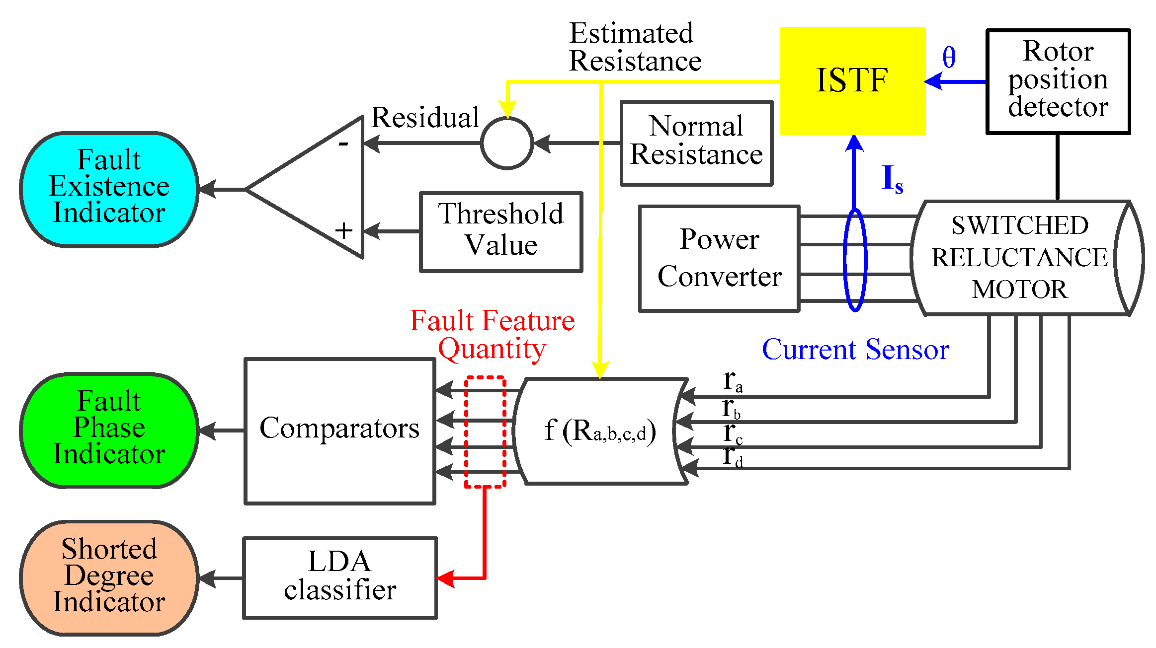
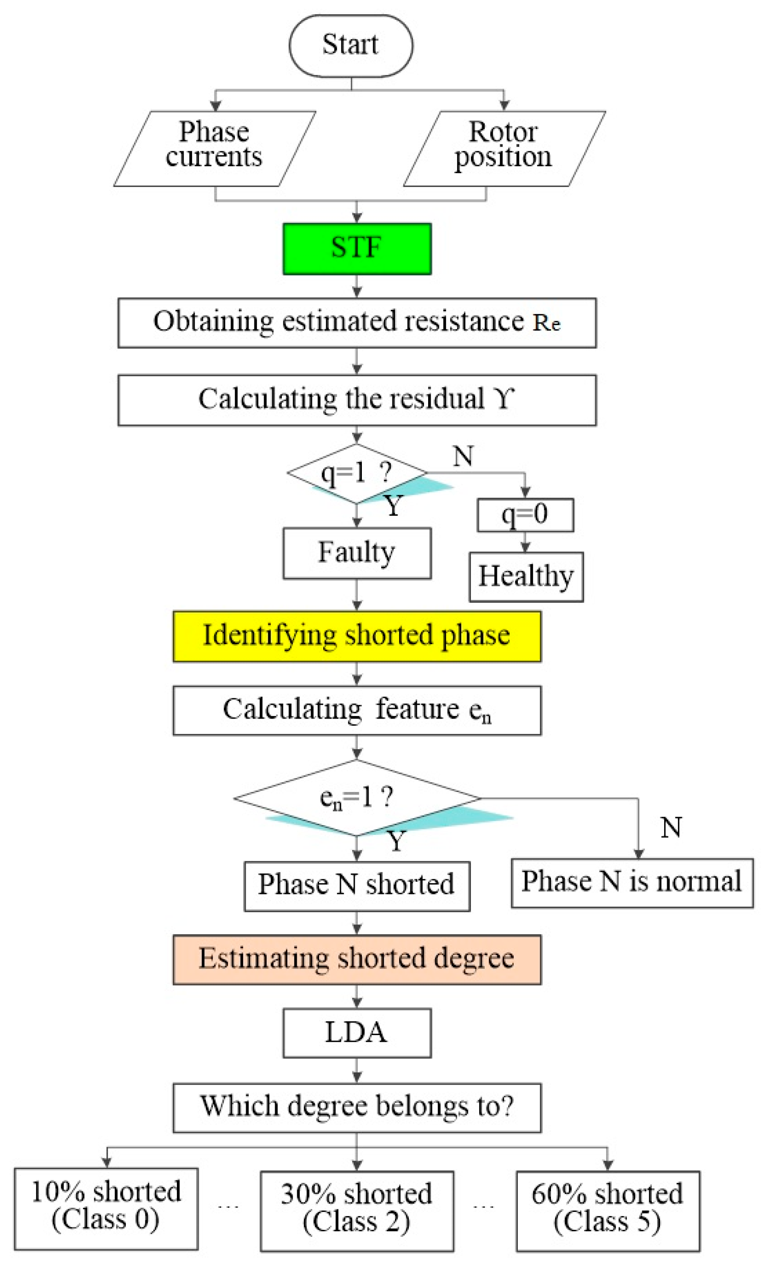
4. The Proposed Fault Diagnosis Method for Inter-Turn Shorted-Circuit Fault (ISCF)

The measurement variables included the measured rotor angles and the real-time four phase currents should be required to send the STF. While the resistance of the machine’s phase windings, can be calculated by STF. The schematic of the proposed detection method is shown in Figure 3. It can be noted that the whole diagnosis program contains detection of the fault occurrence, identifying the faulty phase and estimation of faulty severity.

4.1. Detecting the Occurrence of ISCF

The proposed diagnostic method depends on the estimation of phase winding resistances. According to explanations in Section 2 and Reference [15], the conclusion that the faulty phase winding resistance must be decrease, has been already confirmed. However, in the SRM’s normal operation, the phase winding resistances always increase with the temperature of winding goes up. Thus, the variation of the winding resistance can be tracked by the STF to diagnose the fault occurrence. The specific process is as follows.
The rotor position and four phase currents are applied to obtain the normalized estimated resistance Re based on the algorithm STF. Comparing Re and the normalized normal resistance Rr to generate the residual ϒ. Any important differences between the resistance Re and Rr indicates that the ISCF occurs in the machine’s winding. The diagnostic feature quantity q is defined as follows:
q = {   1 ,   i f   | ϒ | > R ref   0 ,   i f   | ϒ | R ref
In the experimental tests, Re and Rr present some differences, even during normal operation. A part of these differences results from transient phenomena, as well as another part is brought from signal noises enrolled by sensors. To avoid a wrong fault diagnosis caused by above undesirable effects, a threshold value Rref is considered. In any situations, Rref must be clearly higher than the maximum absolute value of Υ.
When q is equal to 1, it means that absolute value of ϒ is higher than Rref. This scenario occurs if the ISCF in one or more phase windings. When q is equal to 0, it means that Υ lies in the normal range, that can indicate the normal operation of SRM.

4.2. Identifying the Faulty Phase

The voltage for each phase is expressed by Equation (56) during the phase is in the turn-on region.
U n = { U s ,   upper-switch close & & lower-switch close   0   ,   upper-switch open & & lower-switch close
where Us represents the dc voltage. When the two switches of one phase on the power converter are all close, the normal phase voltage Un is equal to the Us.
Once the ISCF occurs, the amplitude of the faulty phase current is surely higher than the normal value, yet currents of the remaining normal phases should be not influenced by the ISCF due to the independence of each phase winding, which results that the amplitude of Rr·in is also greater than the normal phase voltage Un during the faulty phase is in the turn-on region. Thus, the characteristic of phase voltage, which of the faulty phase in the turn-on region can be used to diagnose the shorted phase. The diagnostic variables gn and en are introduced to identify the faulted phase, which can be defined as:
g n = { | U s R r i n |   ,   i n 0   and   U s 0 1   ,   i n = 0   or   U s = 0
where n = A, B, C, D. To identify easily, the diagnostic variables gn would be set as the value of 1 during the phase n in the turn-off region. The diagnostic variable en is Boolean, installed as:
e n = { 0 ,   i f   g n 1 1 ,   i f   0 < g n < 1
When en is equal to 1, the phase n is indicated as the shorted phase. However, this only concerned if the variable q is also equal to 1 simultaneously, as shown in Table 1.
If there is only one en variable would be equal to 1, then just one phase is faulty. More than one en variable presents the value 1, which means the number of faulty phases is greater than 1. In other words, the number of en variable presented the value 1 can indicate the number of the faulty phase. The variables for multiphase ISCF are presented in Table 2 by taking faulty phase C as an example.

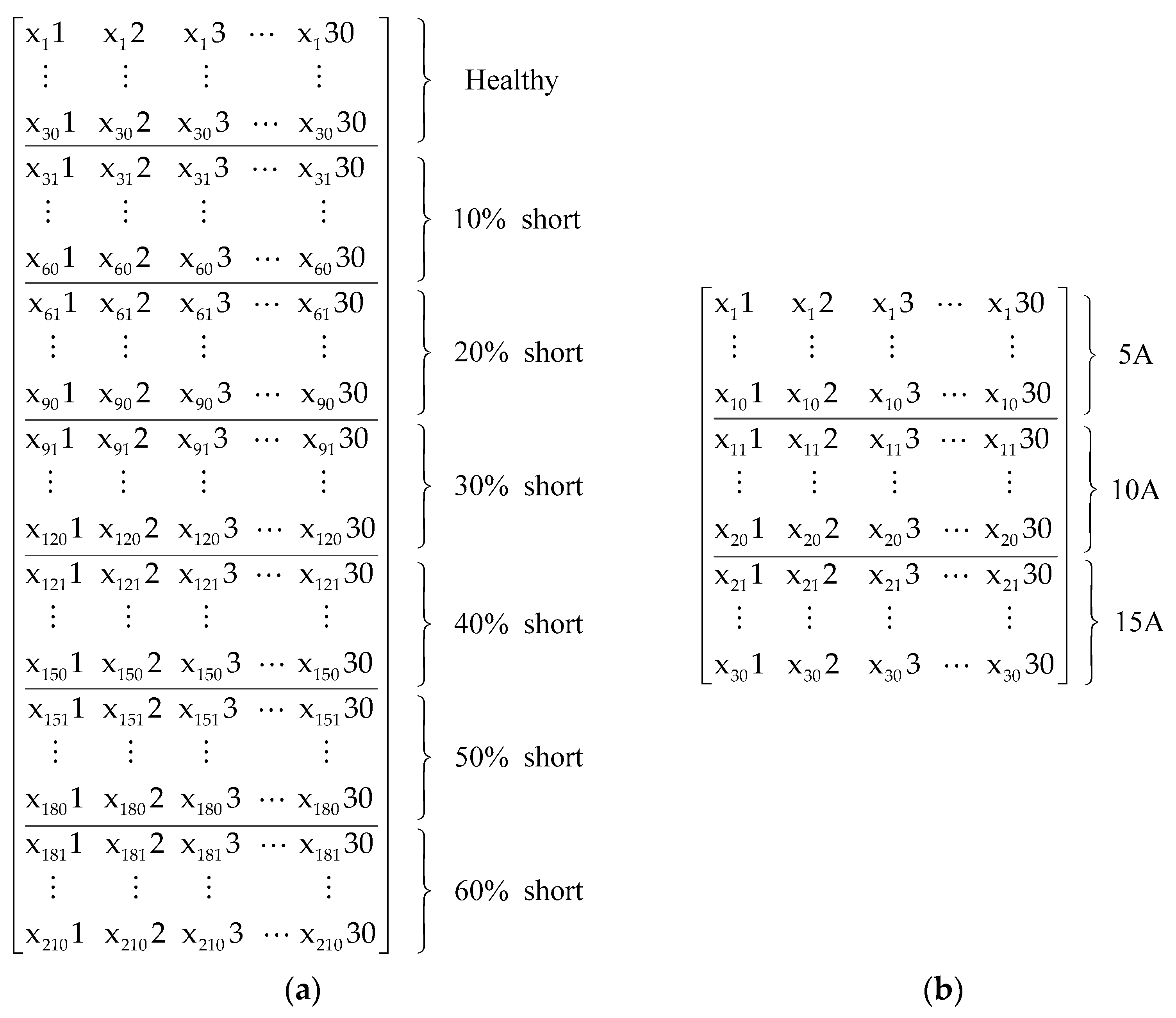
4.3. Estimation of Fault Severity

It is necessary to estimate the fault degree, after the fault and its type are all identified. The LDA classifier is applied to detect the faulty degree. In the LDA classifier, samples from the faulted prototype with different severities are involved in the sample space, where the space is divided into k classes. A certain number of samples within the same condition are classified into the same class. Each class is related to the weighting coefficient, which is utilized to compute the corresponding linear discriminant function (LDF) [21]. The LDF for the kth class is expressed by:
C k ( X i ) = α 1 k x i 1 + α 2 k x i 2 + L + α N k x i N + α ( N + 1 ) k
where [α1k, α2k, …, α(N + 1)k] is the coefficient matrix of the kth class. and the N dimensional vector for the sample Xi is represented by Xi = [xi1, xi2, …, xiN].
For each iterative process, the weighting coefficient matrices can be resolved during the samples training. The k × N matrix is firstly guessed arbitrarily and the weighting coefficient matrix should be revised in each iteration. The class k of the training sample Xi is known, yet the coefficients are always adjusted till that the LDF Ck (Xi) for the kth class is bigger than for the other classes. In case the training procedures are all finished, as well as the matrix C has been achieved, the discriminant functions for the unclassified sample are computed to obtain the optimal coefficient. If the LDF for one sample is bigger than any other LDF, then this sample vector could be classified to a specific class. An unknown sample vector i can be classified to the class j if:
C j ( X i ) C k ( X i ) j k
To verify the effectiveness of the presented method over the widespread running range, but not just at special case, the sampling space resistance is abounded to contain different operation speeds and currents in this section. The training matrix contains seven classes, respectively representing different faulty degrees (0–60%). In each class, the space includes 30 samples, corresponding to currents with different levels (5A,10A,15A). Each current level includes 10 samples, which are created by varying the amplitude of the speed from 600 r/min to 1500 r/min in the step of 100 r/min. Thus, the training matrix is generated by the overall 210 samples. The association of the estimated resistance at different rotor positions from 0–30° are utilized to classify the faulty severity by LDA. The full structure of training matrix for different shorted degree is shown in Figure 4a. The structure of the training matrix for healthy case is shown in Figure 4b.
Additionally, the leave-one-out method is used to verify the faulty degree estimated method. Firstly, only one sample is chosen and taken as the leftover sample. The other samples are used to calculate the coefficient matrix. Afterwards, the chosen sample is classified by the trained well coefficients. Then this classification procedure is duplicated for each sample. Thus, the coefficients are recomputed and the left-out sample is classified by these coefficients again and again. The accuracy of estimated faulty degree for each class could be expressed as:
degree ( % ) = N correct N all × 100 %
where degree (%) indicates the percentage of the correct classification for every class, Ncorrect is the number of the classified correctly samples, Nall is the total number of samples.

5. Simulation and Experimental Results

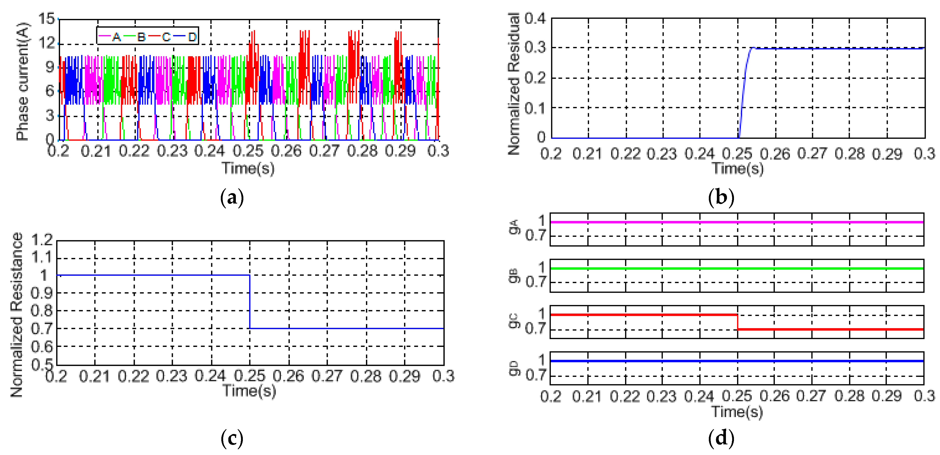
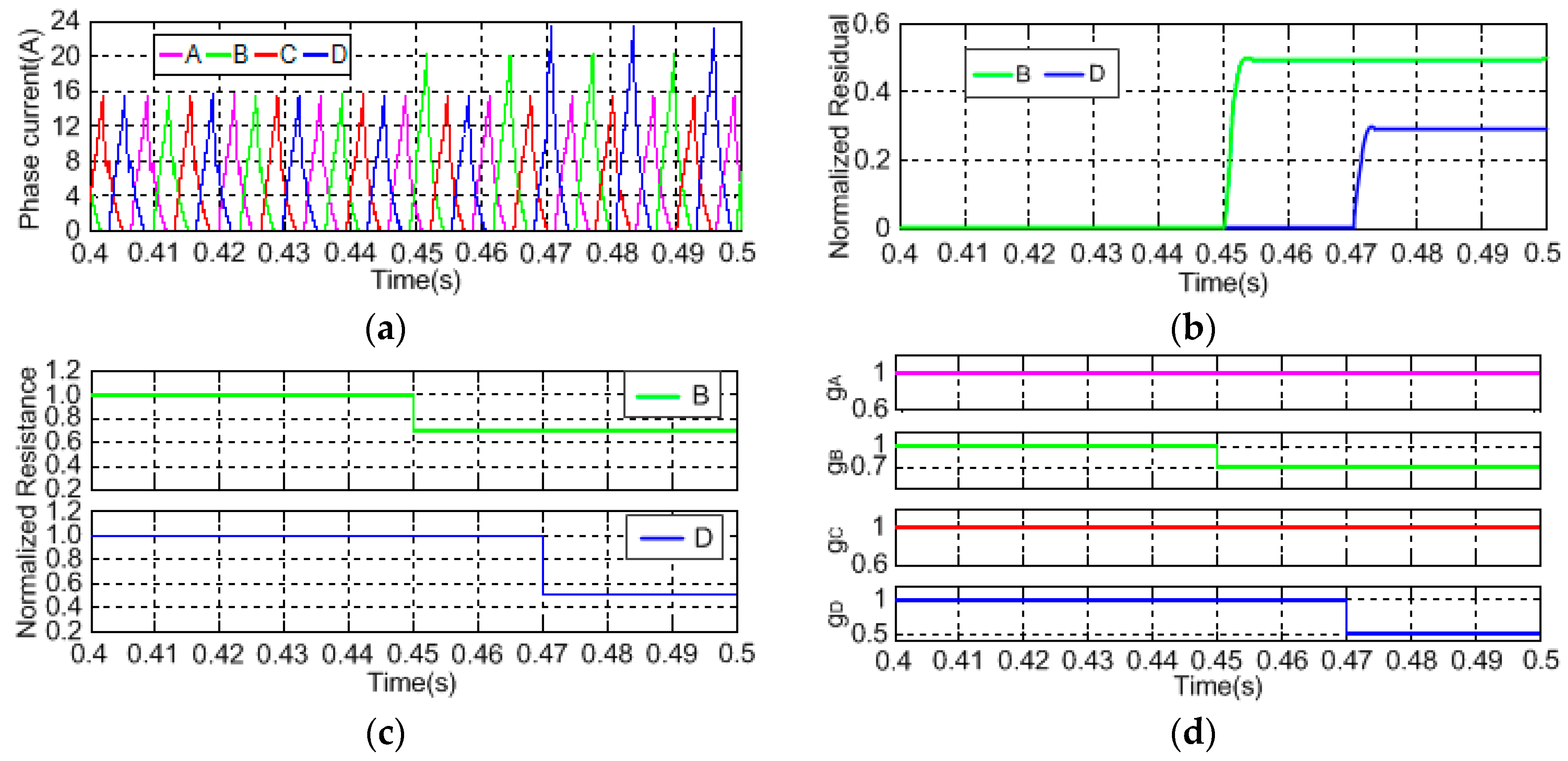
5.1. Simulation Analysis

A simulation model for the fault diagnosis method was built based on Ansys Maxwell and Matlab/Simulink. The SRM model is set up in Ansys/Maxwell based on Finite Element Analysis (FEA) while the control part and fault diagnostic part are all found in Matlab/Simulink. Different shorted-circuit turns of the phase winding can be easily sited in Maxwell. The flow diagram for the diagnosis algorithm is shown in Figure 5.
To confirm the performance of the ISCF diagnostic method, a lot of simulation and experiments were carried out corresponding to different speed and load running status. For this purpose, the unfavorable scenarios are considered, which correspond to the no-load and loading operations. Moreover, different scenarios including only one phase failure and multiphase failure are, respectively, discussed and tested in this section. The SRM characteristics are detailed in Table 3.
Figure 6 presents the simulation results for 30% turns shorted in which 120 turns of the phase winding are faulty. Four phase currents, the normalized residual, the normalized resistance and diagnostic variables gn are respectively shown in this figure, which correspond to the 600r/min steady-state and no-load operation. At 0.25 s, 30% turns fault related to phase C was imitated. After the ISCF occurrence, the magnetization of shorted turns for phase C is not possible anymore, and phase C current immediately goes up. Then, it is registered an obvious difference between Re and Rr, and the normalized residual γ changes from 0 till 0.3 (Figure 6b), which is higher than the threshold value Rref, as well as the normalized resistance decreases from 1 to about 0.7 (Figure 6c). According to Equation (55), the variable q is equal to 1, indicating a possible ISCF appearance.
Simultaneously, the variable gC presents sudden change at 0.25 s, while diagnostic variables gA, gB, gD are all throughout equal to 1 (Figure 6d). According to Equation (58), the diagnostic variables eA = eB = eD = 0, eC = 1 and ∑en = 1. Therefore, the ISCF associated to phase C is quickly diagnosed due to eC = 1 and it is only variable equal to 1. In the fault diagnostic procedure, the threshold value Rref is especially important. In this paper, Rref is defined as 0.05 based on several experimental tests.
The applicability and extendibility of the proposed fault diagnostic method for more than one phase failure was tested exposing the SRD with the speed at 1500 r/min and loading 3 N·m. Figure 7 presents simulation results for windings of phase B and D respectively with 30% and 50% turns fault. The winding of phase B failure occurs at 0.45 s, soon afterwards the winding of phase D shorted at 0.47 s. After the fault occurrence, the magnetization of shorted turns for phase B and D vanish, and currents of phase B and D also increase (Figure 7a). Moreover, there is an obvious difference between Re and Rr, resulting in generating the normalized residual Γ of phase B and D, that are all higher than the threshold value Rref (Figure 7b). Then the normalized resistance of phase B decreases from 1 to about 0.7 and the normalized resistance of phase D decreases from 1 to about 0.5 (Figure 7c). Thus, the diagnostic variable q is equal to 1, proving an ISCF occurrence. Meanwhile, it can be noted that the variables gB, gD present sudden change respectively at 0.45 s and 0.47 s, yet the variables gA, gC remain unchanged (Figure 7d), thereby the variables eA = eC = 0, eB = eD = 1 and ∑en = 2. Thus, the ISCF associated to phase B and phase D can be quickly diagnosed.

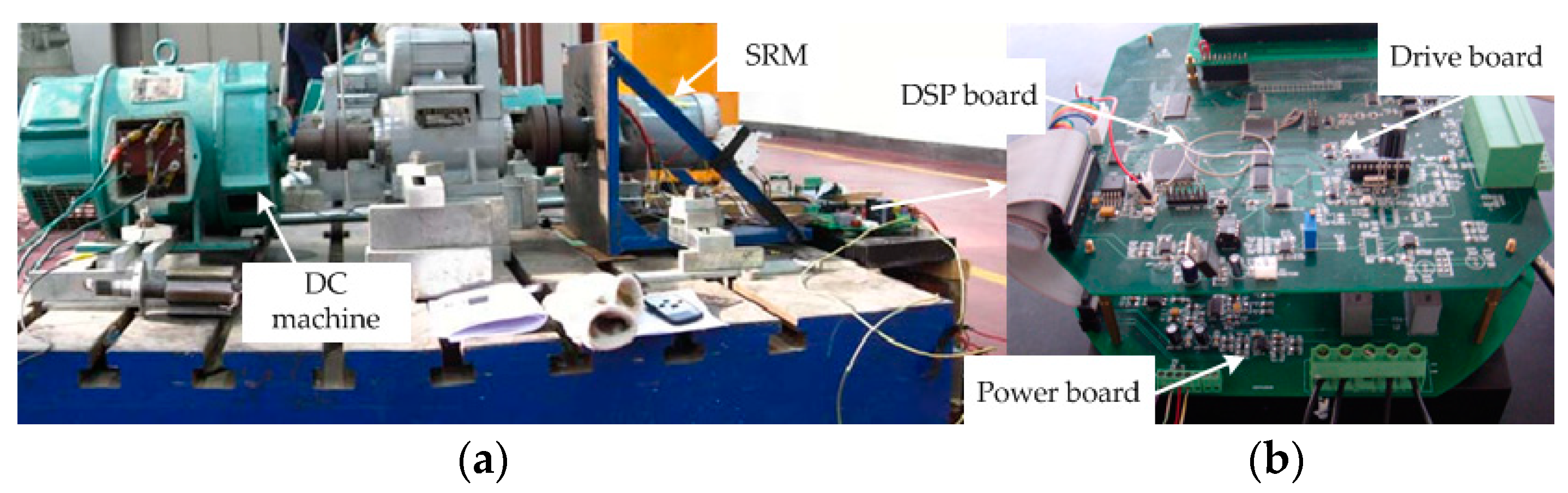
5.2. Experimental Results

To verify the advanced diagnostic method by experimental teats, an experimental platform was set up, as shown in Figure 8. Experiments were developed on the prototype. An asymmetric half-bridge converter is employed. The control procedure based on current chopping control (CCC) and angle position control (APC), as well as the diagnostic program, is executed in the DSP TM320F2812. This digital signal processor is utilized as the primary control chip corresponding with high speed logic circuit.
Figure 9 shows the phase current iC, the normalized residual, diagnostic variables gC and the real-time speed before and after 30% turns of the phase C failure, at 600 r/min, with no-load. The resistance Re is generated on phase currents and rotor positions by the STF algorithm. Due to the ISCF, there is an obvious difference between Re and Rr, leading to the amplitude of normalized residual goes up suddenly and the variable gC is smaller than the value of 1, that means q = 1, eC = 1 and ∑en = 1. Therefore, the ISCF only associated to phase C can be quickly diagnosed at 1.08 s.
Figure 10 presents the phase currents, normalized residual, diagnostic variables and the real-time speed before and after 30% turns winding of phase B and 50% turns winding of phase D failure. An angle position control algorithm is conducted during the high speed operation. To verify the robustness of the advanced method, the load changes from 0 N·m to 3 N·m suddenly at 3.1 s and the speed is 1500 r/min. After 3.1 s, the phase currents B and D almost raise from 8 A to 16 A due to the load rising, while the normalized residual B and D are still approximately keep the value of 0 and diagnostic variables gB, gC, and gD are all approximately 1 because the phase windings are healthy. However, at 3.3 s, the amplitude of phase current ib changes to about 24 A, and the normalized residual B and the variable gB also vary substantially. Subsequently, the amplitude of the current id also increases to about 24 A at 3.4 s. The normalized residual D goes up and the variable gD decreases suddenly at the same time. Actually, at high speed and variable load, an ISCF also causes a significant difference between Re and Rr. Diagnostic variables q = 1, eA = eC = 0, eB = eD = 1 and ∑en = 2, that are exported to diagnostic results. It is clearly indicated that the ISCF appears in the phase B and D.
After diagnosing the fault occurrence and faulty phase, it is necessary to estimate the severity by LDA.
The simulation and experimental results of faulty severity for the SRM with different loads are shown in Table 4. From the results, it is obvious that LDA can also validate the occurrence of the ISCF and estimate the faulty severity, as well as the accuracy reaches up to above 95%. But, some of the samples related to the 10% ISCF are not classified precisely, not only the simulation results but also the experimental results.

6. Conclusions

Safety and reliability are the most significant property indicators for SRD-based electric vehicle applications. In this article, a new diagnosis method of stator ISCF was proposed for SRMs. To improve the detection preciseness further, the resistance of the phase windings was chosen as the diagnostic feature. Since the STF has the superior tracking performance, the diagnosis scheme used the STF to track the real-time resistance of the phase windings, so as to obtain the resistance differences between the healthy phase winding and the faulty phase winding. Then, the resistance differences comparing with the threshold were utilized to detect the fault occurrence and the faulty phase, as well as the number of faulty phases could be also diagnosed. Specifically, LDA was employed to estimate the faulty severity but not identify the faulty type based on the resistances corresponding to different phase currents and rotor positions with the severity from 0% to 60%. Finally, a large number of simulation studies and experiments were executed to validate the robustness and accuracy of the presented method. Whether the SRM was running at low speed or high speed, the accurate diagnostic results can be received with one current period. As further work, the performance of the advanced method in the event of a sudden load change suddenly has been discussed. The results can certify the accuracy and rapidity of the advanced diagnosis method in this case, while the future work is to further improve the precision of the estimating severity by the improved Linear Discriminant Analysis.

Author Contributions

L.X. and H.S. provided the key discussions and ideas for the paper. L.Y. and X.R. built the setup and experimental implementations, the script was composed by L.X., H.S., L.Z., and F.N. revised and reviewed the script.

Funding

This work is supported by Natural Science Foundation of Tianjin (16JCQNJC04200), the National Natural Science Foundation of China (51637009 and 51707174), the National Natural Science Foundation for nurturing of Tianjin University of Commerce (No. 160123), and the University Students Innovation and Entrepreneurship Training Program of China (201810069019 and 201810086136).

Conflicts of Interest

The authors declare no conflict of interest.

References

  1. Bruno, L.; Suresh, G.; Avoki, M.O. Winding short circuits in the switched reluctance drive. IEEE Trans. Ind. Appl. 2005, 41, 1178–1184. [Google Scholar]
  2. Suresh, G.; Avoki, M.O.; Bruno, L. Classification and remediation of electrical Faults in the switched reluctance drive. IEEE Trans. Ind. Appl. 2006, 42, 479–486. [Google Scholar]
  3. Rareş, T.; Ioana, B. Effects of winding faults on the switched reluctance machine’s working performances. In Proceedings of the 3rd IEEE International Symposium on Logistics and Industrial Informatics, Budapest, Hungary, 25–27 August 2013. [Google Scholar]
  4. Dorrell, D.G.; Makhoba, K. Detection of Inter-Turn Stator Faults in Induction Motors Using Short-Term Averaging of Forward and Backward Rotating Stator Current Phasors for Fast Prognostics. IEEE Trans. Magn. 2017, 53, 1–7. [Google Scholar] [CrossRef]
  5. Obeid, N.H.; Boileau, T.; Nahid-Mobarakeh, B. Modeling and Diagnostic of Incipient Inter-turn Faults for a Three-Phase Permanent Magnet Synchronous Motor. IEEE Trans. Ind. Appl. 2016, 52, 4426–4434. [Google Scholar] [CrossRef]
  6. Cuevas, M.; Romary, R.; Lecointe, J.P.; Jacq, T. Non-Invasive Detection of Rotor Short-Circuit Fault in Synchronous Machines by Analysis of Stray Magnetic Field and Frame Vibrations. IEEE Trans. Magn. 2016, 52, 1–4. [Google Scholar] [CrossRef]
  7. Jawadekar, A.; Paraskar, S.; Jadhav, S.; Dhole, G. Artificial neuralnetwork-based induction motor fault classifier using continuous wavelet transform. Syst. Sci. Control Eng. 2014, 2, 684–690. [Google Scholar] [CrossRef]
  8. Rodríguez, P.V.J.; Arkkio, A. Detection of stator winding fault in induction motor using fuzzy logic. Appl. Soft Comput. 2007, 8, 1112–1120. [Google Scholar] [CrossRef]
  9. Abiyev, R.; Kaynak, O. Fuzzy wavelet neural networks for identification and control of dynamic plants-a novel structure and a comparative study. IEEE Trans. Ind. Electron. 2008, 55, 3133–3140. [Google Scholar] [CrossRef]
  10. Li, X.; Sun, H. Analysis and research of short-circuit fault for SRD based on Maxwell and simplorer. In Proceedings of the 4th International Conference on Manufacturing Science and Engineering, Dalian, China, 30–31 March 2013. [Google Scholar]
  11. Chen, H.; Han, G.; Yan, W.; Lu, S.; Chen, Z. Modeling of a Switched Reluctance Motor Under Stator Winding Fault Condition. IEEE Trans. Appl. Supercond. 2016, 26, 1–6. [Google Scholar]
  12. Torkaman, H. Intern-turn short-circuit fault detection in switched reluctance motor utilizing MCPT test. Int. J. Appl. Electromagn. Mech. 2014, 46, 619–628. [Google Scholar]
  13. Hoseini, S.R.K.; Farjah, E.; Ghanbari, T.; Givi, H. Extended Kalman filter-based method for inter-turn fault detection of the switched reluctance motors. IET Electr. Power Appl. 2016, 10, 714–722. [Google Scholar] [CrossRef]
  14. Xiao, L.; Sun, H.; Gao, F.; Hou, S.; Li, L. A New Diagnostic Method for Winding Short-Circuit Fault for SRM Based on Symmetrical Component Analysis. Chin. J. Electr. Eng. 2018, 4, 74–82. [Google Scholar]
  15. Aubert, B.; Regnier, J.; Caux, S.; Alejo, D. Kalman-Filter-Based Indicator for Online Inter turn Short Circuits Detection in Permanent-Magnet Synchronous Generators. IEEE Trans. Ind. Electron. 2015, 62, 1921–1930. [Google Scholar] [CrossRef]
  16. Nadarajan, S.; Panda, S.K.; Bhangu, B.; Gupta, A.K. Online Model-Based Condition Monitoring for Brushless Wound-Field Synchronous Generator to Detect and Diagnose Stator Windings Turn-to-Turn Shorts Using Extended Kalman Filter. IEEE Trans. Ind. Electron. 2016, 63, 3228–3241. [Google Scholar] [CrossRef]
  17. Liu, M.; Zhou, D.H. Normalized residuals based strong tracking filter and its application. Proc. CSEE 2005, 25, 71–75. [Google Scholar]
  18. Yu, W.; Zhao, C. Sparse Exponential Discriminant Analysis and Its Application to Fault Diagnosis. IEEE Trans. Ind. Electron. 2018, 65, 5931–5940. [Google Scholar] [CrossRef]
  19. Mbo’o, C.P.; Hameyer, K. Fault Diagnosis of Bearing Damage by Means of the Linear Discriminant Analysis of Stator Current Features from the Frequency Selection. IEEE Trans. Ind. Appl. 2016, 52, 3861–3868. [Google Scholar] [CrossRef]
  20. Li, W.; Zhao, C.; Gao, F. Linearity evaluation and variable subset partition based hierarchical process modeling and monitoring. IEEE Trans. Ind. Electron. 2018, 65, 2683–2692. [Google Scholar] [CrossRef]
  21. Reemon, Z.H.; Elias, G.S. On the Accuracy of Fault Detection and Separation in Permanent Magnet Synchronous Machines Using MCSA/MVSA and LDA. IEEE Trans. Energy Convers. 2016, 31, 924–934. [Google Scholar]
Figure 1. The structure of switched reluctance machine (SRM).
Energies 12 00134 g001
Figure 2. The equivalent circuit of the coil.
Energies 12 00134 g002
Figure 3. The schematic of the proposed detection method. STF: strong track filter; LDA: linear discriminant analysis.
Energies 12 00134 g003
Figure 4. The structure of training matrix (a) full training matrix for different degree faults; and (b) training matrix for healthy case.
Energies 12 00134 g004
Figure 5. Flow diagram for the inter-turn shorted-circuit fault (ISCF) diagnosis and identification.
Energies 12 00134 g005
Figure 6. Simulation results in case of 30% turns fault of the SRM winding at low speed and no-load (a) four-phase currents; (b) normalized residual; (c) normalized resistance; and (d) diagnostic variables gn.
Energies 12 00134 g006
Figure 7. Simulation results in case of multiphase ISCF with high speed and variable loading. (a) four-phase currents; (b) normalized residual; (c) normalized resistance; and (d) diagnostic variable gn.
Energies 12 00134 g007
Figure 8. Experimental platform: (a) overall test bench; and (b) drive control and fault diagnosis sections.
Energies 12 00134 g008
Figure 9. Experimental results for 30% turns of the motor winding faulty at low speed and no-load.
Energies 12 00134 g009
Figure 10. Experimental results in the case of a multiphase winding fault of the SRM at high speed and variable loading (a) phase currents ib and id, normalized residual of phase B and D; and (b) diagnostic variables gB, gC and gD.
Energies 12 00134 g010
Table 1. Diagnostic variable for identifying the faulty phase.
Diagnostic VariablePhase Winding StatusFaulty Phase
qeAeBeCeD∑en
110001ISCFA
101001ISCFB
100101ISCFC
100011ISCFD
0-----Normal-
ISCF: inter-turn shorted-circuit fault.
Table 2. Diagnostic variable for the phase winding short-circuit.
Diagnostic VariableFaulty NumberFaulty Phase
qeAeBeCeD∑en
1001011C
1101022A C
1111033A B C
1111144A B C D
Table 3. Switched reluctance machine (SRM) characteristics.
ParameterValueParameterValue
Number of phases4rated voltage of the supply220 V
Number of stator poles8number of rotor poles6
Resistance of normal phase4 Ωturn number of each phase120 turns
Rated power1500 Wrated speed1500 r/min
Table 4. Results of identifying fault degree by linear discriminant analysis (LDA) classification.
Faulty DegreeCorrect Classification
Simulation ResultsExperimental Results
No-Load50% Full LoadNo-Load50% Full Load
Healthy100%100%100%100%
10%97%97%95%95%
20%100%99%97%97%
30%100%100%99%99%
40%100%100%100%100%
50%100%100%100%100%
60%100%100%100%100%

